Feasibility Study on Downhole Gas–Liquid Separator Design and Experiment Based on the Phase Isolation Method

Abstract

As oil exploitation enters its middle and late stages, formation pressure drops, and crude oil degases. In production profile logging, the presence of the gas phase will affect the initial oil–water two-phase flowmeter’s flow measurement results. In order to eliminate gas-phase interference and reduce measurement costs, we designed a downhole gas–liquid separator (DGLS) suitable for low flow, high water holdup, and high gas holdup. We based it on the phase isolation method. Using a combination of numerical simulation and fluid dynamic measurement experiments, we studied DGLS separation efficiency separately in the two cases of gas–water two-phase flow and oil–gas–water three-phase flow. Comparative analysis of the numerical simulation calculation and dynamic test results showed that: the VOF model constructed based on $k-\epsilon$ the equation is nearly identical to the dynamic test, and can be used to analyze DGLS separation efficiency; the numerical simulation results of the gas–water two-phase flow show that when the total flow rate is below 20 m³/d, the separation efficiency surpasses 90%. The oil–gas–water three-phase’s numerical simulation results show that the oil phase influences separation efficiency. When the total flow rate is 20 m³/d–50 m³/d and gas holdup is low, the DGLS’s separation efficiency can exceed 90%. Our experimental study on fluid dynamics measurement shows that the DGLS’s applicable range is when the gas mass is 0 m³/d~15 m³/d, and the water holdup range is 50%~100%. The research presented in this article can provide a theoretical basis for the development and design of DGLSs.

1. Introduction

As one of the world’s three major energy sources, oil reserves and production have an effect on many countries’ economic development. Petroleum is a non-renewable energy source. With the increase in demand, petroleum reserves will decrease year by year. As such, the efficient development of petroleum resources has become a crucial research direction in many countries. Oil production in China is dependent on the exploitation of onshore oilfields. Fluid production profile logging technology [1,2] is a key link in oilfield production. Providing oil–water stratified production is integral to the efficient development of oilfields. However, during the high water-cut development period, formation pressure declines, natural gas is freed from the oil, and the wellbore is a three-phase flow of oil, gas, and water (the oil, gas, and water mixture flows upward under the aid of mechanical exploitation, and the gas exists in a free state). If we continue to use the original oil–water two-phase flow logging technology to measure the oil–gas–water three-phase flow, significant measurement errors are inevitable [3]. The gas phase has become one of the main problems affecting output profile measurement accuracy. In recent years, logging technology platforms built by overseas companies such as Schlumberger have explored the measurement of oil–gas–water multiphase flow in oil wells. However, most Chinese oil wells have low fluid production. Due to the uneven distribution of oil–gas–water multiphase flow distribution, and the slippage effect between the phases at low flow rates, it is difficult to measure the three-phase flow’s split-flow rate.

At present, most of the mature flowmeters in oil fields have high measurement accuracy for oil–water two-phase flow. However, if there is interference from the gas phase, it will affect the flowmeter’s measurement accuracy. For example, the measurement principle behind an electromagnetic flowmeter is treating the water phase as a conductive phase and the oil phase as a non-conductive phase. The conductive phase cuts off the magnetic line of force and induces electromotive force. If there is a gas phase, it will reduce the volume holdup in the water phase and increase the oil phase’s volume holdup, so that the measured flow rate is inaccurate. Wang et al. [4] studied the effect of air bubbles on electromagnetic flowmeters’ response characteristics. For conductance sensors, a gas phase will also affect the measurement. Zhai et al. [5] designed a dual-sensor multi-electrode conductance probe to measure the flow parameters of gas–liquid two-phase flow. However, these methods all require the design of a new type of flowmeter, which balloons flow measurement costs. However, phase isolation can be achieved without changing the original sensor structure, and only changing the structure of the collection umbrella [6]. This is a far more economical means of measurement.

At present, some exhaust technologies and equipment are suitable for the oilfield industry. For example, the wire mesh gas–liquid separator [7] is an efficient gas–liquid separation device, which is used primarily to separate liquid droplets with a diameter over 5 μm from the gas. Shi et al. [8] conducted a detailed analysis of the wire mesh separator’s separation mechanism. The Chinese standard for designing wire mesh gas–liquid separators only gives corresponding formulas for the finalized structure, but not the calculation formula for separation efficiency [9]. Andre [10] invented a gas–liquid separation method and bottom hole spiral separator with a gas separation hole. Divonsir Lopes [11] invented the automatic level-controlled gas separator, which can separate the gas phase from two mixed phases (the liquid phase and the gas phase). Wang et al. [12] designed a multi-cup equal flow gas anchor to realize gravity degassing by using gas–liquid density difference, however, the slippage effect’s separation efficiency was low. Li [13] designed a new labyrinth air anchor, that is, an air anchor structure that organically combines the principles of gravity and centrifugal separation. Any series can be formed according to the amount of gas in the oil well to realize the efficient separation of oil and gas. In September 2010, China Petrochemical Corporation developed and patented a high-efficiency downhole gas–liquid separator based on the capture gas anchor effect. However, this method is only suitable for large bubbles and high gas content.

A gas anchor that uses the gas cap exhaust effect can separate the liquid inlet and the exhaust hole. This ensures that the exhaust hole only exhausts the body, and it does not enter the liquid. However, this entails stricter requirements for setting the valve. Research on various exhaust methods has overlooked the downhole gas–liquid separator when the total flow is low, high water holdup, and small gas bubble diameter. Therefore, combining the above exhaust methods and actual logging, we have designed a downhole gas–liquid separator (DGLS) based on the phase isolation method. Its primary function is to separate the gas from the liquid. Then the oil–water two-phase flowmeters [14,15,16] can be placed in the liquid channel, which not only reduces the gas’s influence on the flowmeter’s measurement accuracy but also reduces the measurement costs. In multiphase flow, each phase’s holdup is measured via the volume method, and then the DGLS’s gas–liquid separation efficiency can be calculated.

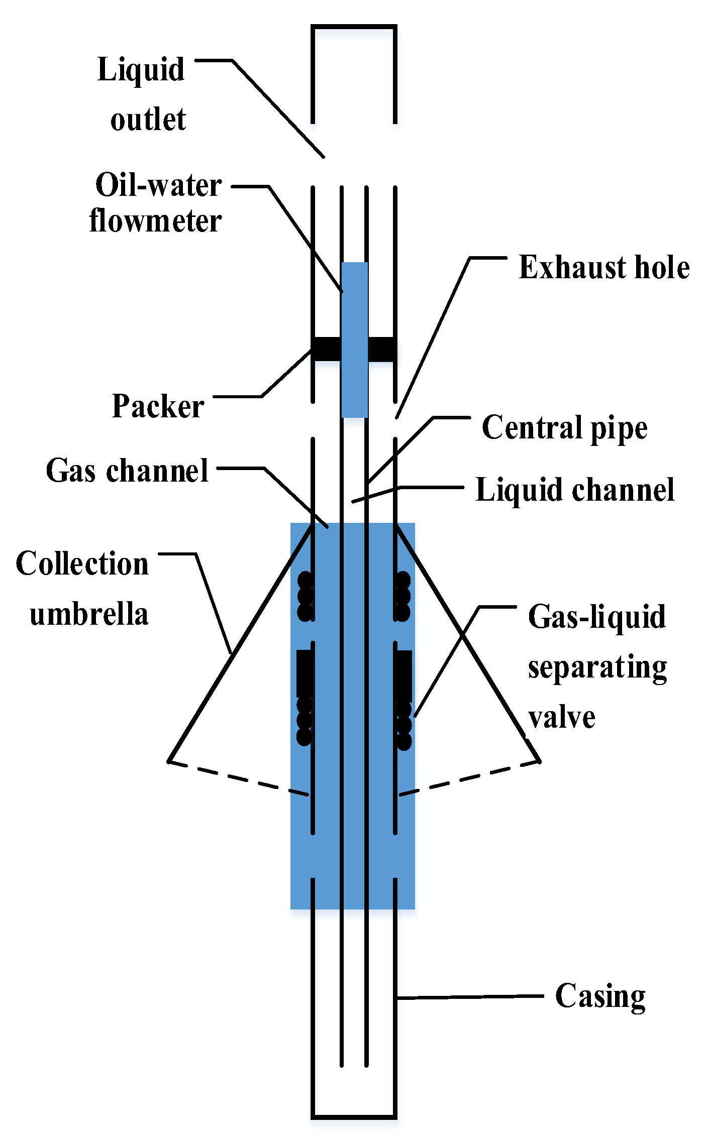
2. DGLS Design

The measuring principle of DGLS is to design a suitable instrument structure to separate the gas phase and liquid phase before the fluid flows through the flowmeter, which is the phase isolation method. The specific method is to install an exhaust valve under the collection umbrella, design a gas circuit and a liquid circuit, and collect the gas under the collection umbrella by using the gas anchor principle to separate the gas and liquid phases. The oil–water two-phase flowmeter is placed in the liquid channel to reduce the gas’s influence on the flowmeter’s output characteristics. Figure 1 shows a schematic diagram of the logging principle. Firstly, the logging tool is lowered into a specific position at the wellhead, and the collection umbrella is opened to fix the logging tool. Then, the fluid flows into the gas–liquid separator from the bottom to the top. Another function of the collection umbrella is to increase flow velocity. The open collection umbrella hinders the fluid’s upward movement and forces it to converge under the umbrella and enter the instrument’s interior through the inlet under the umbrella. According to the orifice outflow in hydrodynamics, the fluid flow rate will multiply, thus increasing the flow rate.

Figure 2 is a profile diagram of the DGLS. The DGLS is composed of a collection umbrella, a gas–liquid separating valve, a central pipe, and a flowmeter for measuring oil–water two-phase. The gas–liquid separating valve separates the gas from the oil–gas–water mixture. The central pipe is used for secondary gas separation. The working principle of the DGLS is as follows: in the annular tubing-casing space, when using a collection umbrella, the oil–gas–water multiphase flow separates. This is due to density differences upon reaching the collection umbrella. Low-density gases first occupy the top of the umbrella to form an accumulation of caps. The crude oil amasses under caps, and water accumulates under reservoirs. As oil–gas–water is produced and accumulates, the gas volume expands downward. When the gas gathers to a certain point, the float control valve opens, and the gas enters through the intake port. It then discharges into the wellbore along the instrument’s central pipe and outer wall. When the oil and water reach the top of the umbrella, the float valve closes, and the above process repeats to achieve the gas–liquid separation effect.

The DGLS’s specific structural parameters are shown in Figure 3. The gas–liquid separating valve is composed of the gas inlet, the float valve, and the liquid inlet. The float valve is connected to the springs and the floater. There are two pairs of springs, one pair is above the floater and the other is below. The floater is composed of stainless steel. The springs are used to offset part of the floater’s gravity. Under normal circumstances, the air inlet remains open. When the upper part of the device fills with gas, the floater remains in the original position, and the gas discharges. When the floater is immersed in the liquid, it rises due to buoyancy, and the gas passage closes. In the small-diameter production profile logging, the instrument structure is affected by the size of the pipe. The main structural parameters of the gas–liquid separating valve are shown in Figure 3.

3. Mathematical Model of Gas–Liquid Separation

The fluid’s phase content will influence the velocity, thus affecting the DGLS’s separation efficiency. The gas–liquid multiphase flow described in this paper includes gas–water two-phase flow and oil–gas–water three-phase flow. Therefore, firstly we established mathematical models of gas–water two-phase flow and oil–gas–water three-phase flow. The phase holdup for each phase can be determined by velocity, and then the gas–liquid separation efficiency can be obtained by calculating the volume content of each phase passing through the DGLS. Finally, we established a mathematical model of the numerical simulation to calculate DGLS’s gas–liquid separation efficiency.

3.1. Characteristic Parameters of Multiphase Flow in Production Profile Logging

In production profile logging, there are three states: oil–water two-phase flow, gas–water two-phase flow, and oil–gas–water three-phase flow. The flowmeter has high measurement accuracy for oil–water two-phase flow. When there are gas–water two-phase flow and oil–gas–water three-phase flow, the existence of the gas phase will affect the measurement accuracy of the flowmeter. Therefore, it is necessary to isolate the gas phase from the liquid phase before measuring the flow of the liquid phase. Next, the separation efficiency of the gas–liquid separator will be analyzed when the fluid medium is gas–water two-phase flow and oil–gas–water three-phase flow.

3.1.1. Gas–Water Two-Phase Flow

Two-phase flow includes gas–water and gas–oil, which is usually called gas–liquid two-phase flow. This paper discusses the problem of gas–water two-phase flow. The calculation formula for the apparent velocity of gas and water in gas–water two-phase flow is [17]:

$${\upsilon }_{sw}=Y_g(C{\upsilon }_m+{\upsilon }_t)$$

(1)

$${\upsilon }_{sg}={\upsilon }_m-{\upsilon }_{sw}$$

(2)

$$C=1.2 ~ 2 \left(usually C=1.2\right)$$

(3)

$${\upsilon }_t=1.53{\left[\frac{{\delta }_{gw}({\rho }_w-{\rho }_g)g}{{\rho }_w{}^2}\right]}^{0.25}$$

(4)

where $C$ is the gas distribution coefficient, ${\upsilon }_m$ is the gas–water mixture’s average velocity, ${\upsilon }_{sg}$ is the gas’s boundary velocity, ${\upsilon }_{sw}$ is the water’s boundary velocity, ${\upsilon }_t$ is the floating velocity of the bubbles in purified water, ${\delta }_{gw}$ is the gas water interfacial tension coefficient, $D$ is the casing’s inner diameter, ${\rho }_w$ is the water density, ${\rho }_g$ is the gas density, $Y_g$ is the proportion of gas in gas water mixture.

3.1.2. Oil–Gas–Water Multiphase Flow

Under the bottom hole condition, the gas’s density is 0.01~0.22 g/cm³. The oil density is 0.6~0.98 g/cm³. The density of water is about 1.0 g/cm³. Therefore, regardless of each item’s contents, the gas flow velocity in the oil–gas–water multiphase flow mixing system is the highest. The water’s flow velocity is the lowest. The oil’s flow rate is between that of gas and water [17].

$${\upsilon }_m={\upsilon }_{sw}+{\upsilon }_{so}+{\upsilon }_{sg}$$

(5)

$$Y_o+Y_w+Y_g=1$$

(6)

$${\upsilon }_{sgw}={\upsilon }_g-{\upsilon }_w=\frac{{\upsilon }_{sg}}{Y_g}-\frac{{\upsilon }_{sw}}{Y_w}$$

(7)

$${\upsilon }_{sow}={\upsilon }_o-{\upsilon }_w=\frac{{\upsilon }_{so}}{Y_o}-\frac{{\upsilon }_{sw}}{Y_w}$$

(8)

$${\upsilon }_{sgo}={\upsilon }_g-{\upsilon }_o=\frac{{\upsilon }_{sg}}{Y_g}-\frac{{\upsilon }_{so}}{Y_o}$$

(9)

After sorting out the above equations, we get the following results:

$${\upsilon }_{sw}=Y_w\left({\upsilon }_m-Y_g{\upsilon }_{sgw}-Y_o{\upsilon }_{sow}\right)$$

(10)

$${\upsilon }_{sg}=Y_g\left[{\upsilon }_m+{(1-Y)}_g{\upsilon }_{sgw}-Y_o{\upsilon }_{sow}\right]$$

(11)

$${\upsilon }_{so}=Y_o\left[{\upsilon }_m-Y_g{\upsilon }_{sgw}+(1-Y_o){\upsilon }_{sow}\right]$$

(12)

and

$${\upsilon }_{so}={\upsilon }_m-{\upsilon }_{sw}-{\upsilon }_{sg}$$

(13)

where ${\upsilon }_{sow}$, ${\upsilon }_{sgw}$ and ${\upsilon }_{sgo}$ are the slippage speed of oil–water, gas–water, and gas–oil, respectively. $Y_g$, $Y_o$ and $Y_w$ are holdup of gas, oil, and water, respectively. ${\upsilon }_{so}$, ${\upsilon }_{sw}$ and ${\upsilon }_{sg}$ are boundary velocities of oil, water, and gas, respectively.

$$C_w=Y_w\left(1-\frac{Y_g{\upsilon }_{sgw}+Y_o{\upsilon }_{sow}}{{\upsilon }_w}\right)$$

(14)

$$C_g=Y_g\left(1+\frac{(1-Y_g){\upsilon }_{sgw}-Y_o{\upsilon }_{sow}}{{\upsilon }_m}\right)$$

(15)

$$C_o=1-C_g-C_w$$

(16)

Equation (14) shows that the higher the flow rate, the more $C_w$ tends toward. In the limit case, it is $C_w\approx Y_w$, $C_o\approx Y_o$, $C_g\approx Y_g$. At the same time, the water holdup is greater than the water content, and the gas holdup is less than the gas content.

In this study, oil, gas, and water are each regarded as incompressible fluids in this paper. Therefore, according to the continuous principle of incompressible fluids, the flow velocity of the fluid entering the instrument through the inlet can be obtained as follows:

$$v_1\Delta S_1=v_2\Delta S_2$$

(17)

where $\Delta S_1$ is the cross-sectional area of Pipe 1, $\Delta S_2$ is the cross-sectional area of Pipe 2,$v_1$ is the velocity through Section 1, and $v_2$ is the velocity through Section 2.

3.1.3. Gas–Liquid Separation Efficiency

In addition to calculating the gas holdup, oil holdup, and water holdup, it is also necessary to calculate the gas–liquid separation efficiency and the oil ratio, for an area in which the volume method is used for measurement. For example, Equation (18) is the calculation formula for gas–liquid separation efficiency.

$${\eta }_g=(1-\frac{\left(1-Y_w\right)*M_a}{Y_{sg}})\times 100\%$$

(18)

where ${\eta }_g$ is the gas collection rate, $Y_w$ is the central pipe’s water holdup, $M_a$ is the central pipe’s total flow, and $Y_{sg}$ is the wellbore’s total gas flow.

$${\eta }_{oil}=\frac{\left(1-Y_w\right)M_a}{Y_{so}}\times 100\%$$

(19)

where ${\eta }_{oil}$ is the oil collection rate ratio, $Y_w$ is the central pipe’s water holdup, $M_a$ is the central pipe’s total flow, and $Y_{so}$ is the wellbore’s total oil. According to the actual engineering needs, ${\eta }_g\ge 90\%$ and ${\eta }_{oil}\ge 90\%$ should be satisfactory.

3.1.4. Laminar and Turbulent

The fluid’s flow pattern can be divided into laminar flow, transition flow, and turbulence. The fluid’s actual flow state of the fluid can be judged according to the Reynolds number. The Reynolds number [18] of a flow in the casing is defined as:

$$\mathrm{Re}=\frac{D\overline{\upsilon }\rho }{\mu }=\frac{D\overline{\upsilon }}{\gamma }$$

(20)

where $D$ is the inner diameter casing (unit: m), $\overline{\upsilon }$ is the average velocity (unit: m/s), $\rho$ is fluid density (unit: kg/m³), $\mu$ is the fluid viscosity (unit: MPa·s), $\gamma$ is the kinematic viscosity (unit: m²/s), and Re is the Reynolds number.

Numerous experiments have shown that Re < 2000 is laminar flow and Re > 4000 is turbulent low. The flow between them is transitional. The value in Equation (21) is determined by the following equation:

$$\overline{\upsilon }=\frac{4q}{\pi D^2}$$

(21)

and therefore

$$\mathrm{Re}=\frac{D\overline{\upsilon }\rho }{\mu }=\frac{\rho {\overline{\upsilon }}^2}{\mu \overline{\upsilon }/D}$$

(22)

where q is the fluid’s mass flow, $\rho \overline{\upsilon }$ is the inertia force, and $\mu \overline{\upsilon }/D$ is the viscous force.

3.2. Establishment of Multiphase Flow Simulation Model

In Fluent, (Version 16.0) there are three kinds of Euler–Euler [19] multiphase flow models: VOF (volume of fluid), mixture models, and Euler models. In order to solve the problem of multiphase flow in this project, it is necessary to ensure the correct flow mode is selected. In this project, we chose the Euler–Euler model because the volume ratio was 1, that is, the volume ratio sum of each phase in the gas–water two-phase flow (or the oil–gas–water multiphase flow) was 1. In the two-phase flow and multiphase flow, the gas’s volume ratio was less than 10%, and thus we adopted the discrete phase model. Since the fluid flow is a type of stratified/free surface flow, we selected a VOF model, a thus established a multiphase flow model. Finally, we performed numerical simulation according to the established model to obtain the required data.

The multiphase flow’s fluid flow can be divided into laminar flow and turbulence. Turbulence [20] models in the Fluent software include the single equation (Splalrt–Allmaras) model, double equation model (Standard $k-\epsilon$ model, RNG $k-\epsilon$ model, Realizable $k-\epsilon$ model), Reynolds stress model, and large eddy model. In Fluent, the turbulent boundary conditions are set as follows:

(a)

Turbulence intensity

The ratio of the velocity fluctuation’s root mean square to average velocity. Less than 1% is low turbulence intensity and at least 10% is high turbulence intensity.

Calculation formula:

$$I\cong 0.16{\left({\mathrm{R}\mathrm{e}}_{{\mathrm{D}}_{\mathrm{H}}}\right)}^{-\frac{1}{8}}$$

(23)

where I is turbulence intensity, and Re is the Reynolds number.

(b)

Turbulence scale and hydraulic diameter

l = 0.07 L,

(24)

where L is the characteristic scale, which can be considered as the hydraulic diameter, and the factor of 0.07 is the maximum mixing length in fully developed turbulent pipe flow. l is the turbulence scale. We selected turbulence intensity and hydraulic diameter for fully developed internal flow.

(c)

Kinetic energy

The most common physical quantity ‘k’ in the turbulence model. Turbulent kinetic energy is estimated by turbulence intensity:

$$k=\frac{3}{2}{\left(uI\right)}^2$$

(25)

where u is the average velocity, and I is the turbulence intensity.

(d)

Turbulent dissipation rate

The turbulent dissipation rate is ε, which is usually estimated by k and turbulence scale l.

$$\epsilon =C_{\mu }^{3/4}\frac{k^{3/2}}{l}$$

(26)

where $C_{\mu }$ is usually 0.09, k is kinetic energy, and l is the turbulence scale.

Through the derivation of the above formula, we can get the standard $k-\epsilon$ model turbulence model settings in Fluent.

4. Data Analysis of Gas–Liquid Separation Efficiency in Two-Phase Flow

Fluent can accurately simulate an experimental target to obtain the parameters of the DGLS. Setting the gas holdup to 10%, the water holdup to 90%, and the total flow of the liquid inlet to be 20 m³/d (‘m³/d’ is the unit of mass flow, i.e., cubic meters per day), 30 m³/d, 40 m³/d, 50 m³/d, 60 m³/d. The actual gas–water two-phase flow and oil–gas–water multiphase flow are complex three-dimensional motion processes. The detailed conditions are set as:

(a)

When fluid flows in a circular pipe, whether it is laminar or turbulent, and its flow has axisymmetric characteristics. This paper focuses on the fluid’s flow characteristics; thus the physical model is simplified into a two-dimensional model in the numerical simulation.

(b)

The inner surface of the vertical riser, the outer surface, and the inner surface of the gas–liquid separation device are ideal smooth surfaces without considering the friction resistance.

(c)

The results show that the fluid flow in the tube is isothermal, the density and viscosity of the fluid are measured at 20 °C, and the gas flow is fully developed laminar or turbulent, unsteady.

(d)

The pressure of velocity inlet pressure is standard atmospheric pressure.

(e)

The measurement error range is ±10% or less.

(f)

In Fluent simulation settings, we set the oil phase to diesel, the gas phase to air, and the water phase to natural water. Water is used as the continuous phase, that is, the first phase.

(g)

The Reynolds number and turbulence intensity are shown in

Table 1. Related parameters of gas–water two-phase flow with 5% and 10% gas holdup.

Gas Holdup	Total Flow (m3/d)	Gas Flow (m3/d)	Water Flow (m3/d)	Reynolds Number	Turbulence Intensity (%)
5%	20	1	19	2514	6.01
	30	1.5	28.5	3771	5.72
	40	2	38	5028	5.51
	50	2.5	47.5	5602	5.44
	60	3	57	7542	5.24
10%	20	2	18	2389	6.05
	30	3	27	3584	5.75
	40	4	36	4779	5.54
	50	5	45	5974	5.39
	60	6	54	7168	5.27

. According to the Reynolds number, 20 m³/d is laminar flow, 30 m³/d is transitional flow, and 40 m³/d~60 m³/d is turbulent flow. There is no calculation model for transition flow in Fluent, and therefore we set the theoretical model of fluid in the transition state as the laminar flow model for solution and calculation.

4.1. Gas–Water Two-Phase Flow Separation Efficiency with 5% Gas Holdup

The DGLS’s gas holdup is 5%, and the water holdup is 95%. The flowmeter is placed in the central pipe. Therefore, as long as the gas holdup in the central pipe is lower than 10% of the total gas holdup at the wellbore inlet, it is considered to meet the engineering requirements. The gas holdup number in the central tube is brought into Equation (19), and then calculated the gas–liquid separation efficiency, i.e., the DGLS’s gas–liquid separation efficiency. As shown in Figure 4, the color chart for the vertical axis shows the phase’s volume content; red indicates that it is 100%, blue indicates that it is 0%. Figure 4a–e show a cloud diagram of the gas phase distribution in the casing when the total flow is 20 m³/d~60 m³/d. Red represents the gas phase and blue represents the water phase. In Figure 4a–d, when the fluid enters the wellbore, most of the gas–water two-phase flow’s flow pattern consists of finely dispersed gas in the water bubble flow (VFD G/W bubble flow). In Figure 4e, most of the gas–water two-phase flow’s flow pattern consists of dispersed gas in water bubble flow (D G/W bubble flow) and VFD G/W bubble flow. When the fluid continues to rise under the collecting umbrella, the stratification of the gas phase and the liquid phase occurs due to the varying density. After the gas phase accumulates to form a gas cap, we opened the exhaust valve and allowed it to enter the exhaust channel, so as to isolate the gas phase and the liquid phase. Then, we discharged the gas phase through the exhaust channel, and the gas–liquid two-phase flow’s flow pattern consisted primarily of bubble flow in water. With the increase in total flow rate, the bubble size at the inlet of the wellbore increased. Additionally, the bubbles discharged through the exhaust channel and gradually expanded but remained part of the G/W bubble flow. At the same time, observation of the central pipe showed that its gas content had also increased along with the increase in total flow.

The simulation analysis results are shown in

Table 2. Gas-water separation efficiency at gas holdup 5%.

Total Flow (m3/d)	20	30	40	50	60
${\eta }_g$(%)	90.5	84.4	79.5	75.1	66.1

through the numerical simulation of the total flow of 20 m³/d~60 m³/d. DGLS can achieve good gas–liquid separation efficiency within the range of 20 m³/d~30 m³/d, and its error is within the allowable range (according to the conditions (e)). With the increase in flow rate, the gas holdup in the central tube also increases. Although the range of gas holdup in the central tube is small, the DGLS’s gas–liquid separation efficiency drops. The larger the total flow rate, the more complex the flow state, and the less pronounced the gas–liquid separation effect. When the flow is 20 m³/d, it can achieve a very high gas–liquid separation efficiency. However, it cannot meet the demand after more than 20 m³/d, and the gas separation effect cannot be achieved at this level.

4.2. Gas–Water Two-Phase Flow Separation Efficiency with 10% Gas Holdup

The gas-phase to water-phase ratio changes without changing the total flow research range. We studied the change in the DGLS’s gas separation efficiency when the gas phase increases. As shown in Figure 5, the gas holdup is 10%, and the water holdup is 90%. With the increase in total flow, the bubble size increases as well. We divided the fluid flow pattern at the inlet into three situations: (1) VFD G/W bubble flow; (2) flow pattern domination by VFD G/W bubble flow with supplemental D G/W bubble flow; (3) flow pattern is supplemented by VFD G/W bubble flow and dominated by D G/D bubble flow. The volume of the gas phase in the central pipe also increases with the increase in the total flow rate. Both the content and the size of the bubbles in Figure 5 are larger than those in Figure 4, and the gas ceiling formation is faster than that in Figure 4. The gas expands, while the gas phase’s volume in the central pipe is also greater than that in Figure 4.

As shown in

Table 3. Gas-water separation efficiency at gas holdup 10%.

Total Flow (m3/d)	20	30	40	50	60
${\eta }_g$(%)	91.2	80.9	75.2	69.1	51.5

, the calculation results for the numerical simulation show that as the total flow increases, the gas–liquid separation efficiency gradually decreases. Only when the total flow rate is 20 m³/d does it meet the condition assumption (e).

Table 2 and Table 3 provide a comparison of the gas–water separation efficiency when the gas content is 5% and 10%, respectively. The DGLS shows a good gas–water separation efficiency at a flow rate of 20 m³/d, and the separation efficiency is similar. When the flow rate exceeds 20 m³/d, the gas–water separation effect is gradually weakened. When the gas holdup is 5% and the flow rate is 30 m³/d~60 m³/d, the separation efficiency is much lower than the gas holdup of 10%. In summary, under the premise of gas–water two-phase flow, the applicable range of DGLS is the total flow rate at 0~20 m³/d. High gas holdup and low flow rates lead to higher gas–water separation efficiency.

5. Data Analysis of Gas–Liquid Separation Efficiency in Multiphase Flow

Section 4 explored the gas–liquid separation efficiency of gas–water two-phase flow. When the oil content is far less than the total content of gas–water two-phases flow, the oil phase is usually regarded as the water phase. However, when the oil phase’ holdup does not meet this condition, the fluid medium must be set as oil–gas–water three-phase flow for simulation research. This section discusses the relevant parameters when the flow medium is oil, gas, or water three-phase flow. The total flow is 20 m³/d, 30 m³/d, 40 m³/d, 50 m³/d, 60 m³/d, and the gas holdup is 5%, the oil holdup is 10% and the water holdup is 85%. When calculating the gas–liquid separation efficiency, we also need to check the oil content in the central pipe. The existing production profile logging technology can measure the flow of two-phase flow, that is, the oil–water flow, and the measurement technology is relatively mature. However, if there is a gas phase, the flowmeter will be less accurate. Therefore, the purpose of this project is to separate the gas from oil–water, so that the original flow can be maintained in order to measure the multiphase flow.

Table 4. Related parameters of oil-gas-water multiphase flow.

Total Flow (m3/d)	Gas Flow (m3/d)	Oil Flow (m3/d)	Water Flow (m3/d)	Reynolds Number	Turbulence Intensity (%)
20	1	2	17	2255	6.095
30	1.5	3	25.5	3383	5.794
40	2	4	34	4511	5.589
50	2.5	5	42.5	5638	5.435
60	3	6	51	6766	5.313

shows the Reynolds number and turbulence intensity under different flow rates.

5.1. Analysis of Numerical Simulation Results of Oil–Gas–Water Multiphase Flow

By numerically simulating the oil–gas–water multiphase flow within the range of 20 m³/d~60 m³/d, the gas holdup is 5%, the oil holdup is 10%, and water holdup is 85%. We obtained the gas holdup, oil holdup, and water holdup in the central pipe via the volume method. Figure 6 is a cloud diagram of gas-phase distribution under different flow rates; red represents the gas phase, and blue represents the water phase. As the flow increases, the gas holdup in the casing increases, and the gas volume under the collection umbrella gradually decreases, while the gas holdup in the central tube gradually increases. The bubbles in Figure 6 are bigger than those in Figure 4 due to the addition of an oil phase in Figure 6. Most of the gas phase flow pattern in the oil gas water three-phase flow consists of fine bubble flow. Therefore, adding the oil phase not only increases the flow pattern’s complexity but also affects each phase’s separation velocity. The observation method shows that the gas separation effect is stronger at lower flow rates.

Figure 7 is a cloud diagram of oil phase distribution under different flow rates. Red represents the oil phase and blue represents the water phase. Due to the low oil content, it is in an oil-in-water state in the figure. As the flow rate increases, the oil volume in the central pipe also increases. Visual observation indicated that the DGLS does not separate the oil from the fluid medium, and oil droplets do not accumulate under the collection umbrella. Rather, the distribution of oil in the central tube is similar to that in the wellbore.

The numerical simulation results are shown in

Table 5. Gas–liquid separation efficiency at oil–gas–water multiphase flow.

Total Flow (m3/d)	20	30	40	50	60
${\eta }_g$(%)	92.4	90.9	90.5	90.4	86.5
${\eta }_{oil}$(%)	91.9	95.3	93.2	99.3	99.1

. When the total flow is between 20 m³/d and 50 m³/d, the gas–liquid separation efficiency can surpass 90%, and the results is meeting the conditional (e) and engineering requirements. With the increase in total flow rate, the gas–liquid separation efficiency decreases gradually, that is, when the total flow rate reaches 60 m³/d, the gas–liquid separation efficiency is the lowest. From the oil collection efficiency in the central pipe, the DGLS can not only isolate the gas and liquid but also ensure the central pipe’s oil holdup. The results show that with the increase in total flow at any time, the oil holdup in the central pipe gradually increases and tends to hold up oil at the inlet. This indicates that the greater the flow, the better the DGLS performs. However, at low flow rates, the oil holdup is the lowest, because the interface between the gas and the oil is not pronounced when oil and gas gather under the umbrella. When the gas–liquid separation valve is opened, the oil phase will also enter the gas channel and discharge. From this point, it cannot enter the central pipe, and so the oil holdup in the central pipe declines. According to the above data analysis, the applicable range of DGLS for oil–gas–water multiphase flow is 20 m³/d~50 m³/d.

5.2. Numerical Simulation of Two-Phase Flow and Multiphase Flow

As shown in Figure 8, DGLS can meet the measurement requirements for the gas–liquid separation efficiency when the total flow is 20 m³/d, regardless of whether the medium is two-phase flow or multiphase flow. Therefore, the numerical simulation of gas–water two-phase flow can be used instead of oil–gas–water multiphase flow, which not only simplifies the model’s settings but also produces the required effect in a shorter time.

When the total flow is 30 m³/d~60 m³/d, the numerical simulation results for gas–water two-phase flow diverge from the numerical simulation results from the multiphase flow. In the process of gas-liquid separation, compared with the numerical gas–water simulation, adding the oil phase into the multiphase flow complicates the interaction between the equation describing the multiphase flow and the gas–liquid. It also increases the fluid flow state’s complexity. Therefore, the numerical simulation results for gas–water two-phase flow cannot replace the oil–gas–water multiphase flow’s numerical simulation results, especially when observing the gas–liquid separation gas volume. According to Equations (1)–(16), with the increase in the oil phase, the slippage effects between oil, gas, and water also increase, changing each phase’s viscosity. With the gradual increase in flow, the slippage effect intensifies, leading to the stratification phenomenon in the gas, oil, and water phases. The oil phase’s viscosity coefficient is greater than that of the water and gas phases, and when the gas enters the gas channel, the oil phase acts as a seal and blocks the water phase. At the same time, the exhaust hole’s tiny diameter hinders the entry of the oil phase. Therefore, the gas–liquid separation efficiency of oil–gas–water three-phase flow is superior to that of gas–water two-phase flow.

6. Dynamic Experimental Research of DGLS

The experimental prototype processed by the principle of phase isolation is used for the dynamic experiment (Dynamic experiment means the fluid is circulating, and the measured data have volatility) on the multiphase flow experimental device, the dynamic response of the instrument is observed and summarized, and the stability of the instrument is verified.

6.1. DGLS Experimental Prototype

According to the design specifications of the optimized method obtained by the simulation results, we manufactured, processed, and installed an experimental prototype of the split structure. The DGLS experimental prototype’s multiphase flow device was composed primarily of a multiphase flow experimental device, an impedance sensor, a turbine flowmeter, and a collection umbrella, as shown in Figure 9. We linked the assembled DGLS experimental prototype to the multiphase flow experimental device, and set flow rates for the gas phase, oil phase, and water phase. The oil, gas, and water enter the DGLS through the oil pipe’s annular space. The turbine flowmeter is used to measure the total flow of oil and water, and the frequency signal is obtained through the surface acquisition device. The fluid passing through the DGLS flows into the storage tank through the phase separation device.

The central pipe’s body is made of plexiglass. The advantage of using this material is that it is non-conductive and strong, and therefore suitable for underground environments. The central pipe is shown in Figure 10. The processed experimental prototype is shown in Figure 11, where the outer diameter of the instrument is 28 mm, and the inner diameter of the flow channel is 10 mm.

6.2. Multiphase Flow Experimental Device

The dynamic experiment was completed on the multiphase flow experimental device of Daqing Oilfield. The multiphase flow experimental device can simulate the actual situation of oil–water mixture flowing in the pipeline during the oil production process, and can intuitively observe that the instrument is in the simulated wellbore. The circumstances and simulation of the flow pattern and the flow pattern of the fluid is in the wellbore. The schematic diagram of the multiphase flow experiment device is shown in Figure 12.

The dynamic experiment was completed in the multiphase flow experimental device in Daqing Oilfield. The multiphase flow experimental device was composed of a simulated wellbore, a derrick, a separator, a pressure stabilizing pipe, a turbine transmitter, a pressure device, a storage tank, and a pipeline gate. The most common media in multiphase flow simulation experiments are diesel, water, and gas. During the dynamic experiment on multiphase flow recovery, our staff used the flow control panel to set the accurate flow required for the experiment. Then, they stably input the flowing medium into the wellbore from the storage tank under the control of the pressure stabilizing pipe. Next, they adjusted, tracked, and distributed the turbine transmitter according to the inflow flow value, so as to keep the flow in the inflow pipe consistent with the set flow. After the fluid is measured by the downhole measuring device, it flows from the wellhead into the separator, and each phase is separated into the original states. It then flows into each storage tank and then circulates into the simulated wellbore to ensure the continuous measurement of the instrument. The data collected after the measurement is transmitted to the computer. Through manual operation, parameters such as fluid flow and moisture content are measured and the dynamic data are monitored in real-time by the display. We then analyze the instrument’s response, record the data, analyze the experimental results, and draw a conclusion. The multiphase flow experimental device has powerful functionality and strong control performance; it can intuitively observe the dynamic changes in the fluid.

6.3. Experiment Research on Oil–Gas–Water Multiphase Flow

The purpose of the dynamic experiment is to verify the feasibility of the DGLS gas–liquid separation efficiency measurement. Figure 13 shows the multiphase flow experimental device based on the phase isolation collection umbrella. Through the experiments on the gas–water two-phase and oil–gas–water multiphase flow, we verified the feasibility of the DGLS instrument’s gas–liquid separation. We also observed the dynamic response law, and determined a reasonable structure and separation efficiency for the DGLS. This laid the foundation for the subsequent structural design of the instrument and its large-scale application in oilfield output profile logging.

In order to investigate the DGSL’s separation effect, we conducted dynamic experimental calibration of the turbine flowmeter under different gas-phase flows in oil–gas–water three-phase flow. In the experiment, the gas flow was 5 m³/d, 10 m³/d, and 15 m³/d, the oil–water liquid flow ranged from 1 m³/d to 60 m³/d, and the water holdup ranged from 50% to 100%.

Figure 14 shows the turbine flowmeter’s response characteristic curve when the gas flow is 5m³/d. The horizontal axis represents the total liquid flow, and the vertical axis represents the turbine flowmeter’s response frequency. The turbine response frequency increases with the increase in total liquid flow, and the output response characteristics do not change with water holdup. Moreover, the curve shows a good phenomenon relationship. This shows that the DGLS isolates the gas and liquid phases.

Figure 15 shows the turbine flowmeter’s response curve when the total gas-phase flow is 10 m³/d. With the increase in the total liquid flow, the turbine’s output still increases linearly. However, the frequency at different water holdups is higher than at pure water. This shows that some gas enters the central pipe, which affects the turbine flowmeter’s output frequency. However, this error is within the allowable range, and therefore the DGLS still provides good gas–liquid separation efficiency.

Figure 16 shows the turbine response curve at a gas flow rate of 15 m³/d. When the total liquid flow exceeds 10 m³/d, the curve shows a good linear relationship, but the response frequency at different water holdups is higher than at pure water. This indicates that a large amount of gas enters the central pipe, which affects the turbine flowmeter’s speed. The turbine’s speed when the medium is gas is different from that of when the medium is liquid. When the gas passes through the turbine flow meter, both the turbine speed and the output frequency increase. When the total liquid flow is less than 10 m³/d, the relationship between flow and frequency is nonlinear. This shows that the DGLS’s gas–liquid separation capacity is poor. The gas phase enters the central pipe instead of discharging through the exhaust channel. The gas phase makes the turbine flowmeter more sensitive to the gas phase, but the sensitivity to the liquid phase decreases. This affects the turbine flowmeter’s output characteristics. When the gas flow surpasses 15m³/d, the DGLS cannot produce a sufficient gas–liquid separation effect. Therefore, to produce the expected effect, the gas flow needs to be no more than 15 m³/d.

Figure 17 shows the turbine flowmeter’s output frequency curve when the gas holdups are 5 m³/d, 10 m³/d, 15 m³/d, and none. Firstly, we measure the turbine flowmeter’s output frequency as the control frequency in the absence of a gas phase. Then, we increased the gas flow. When the gas flow rate was 5 m³/d and 10 m³/d, the curve offset was not pronounced, and with the increase in gas flow rate, the gap between the curve and the pure water increased gradually. This shows that with the increase in total gas flow, there was a drop in the DGLS exhaust effect, and a large amount of gas had entered the central pipe. This affects the measurement of the turbine flowmeter.

Figure 18 shows the output frequency curve of the turbine flowmeter with water holdup 70%, oil holdup 30%, gas holdup of 5 m³/d, 10 m³/d, 15 m³/d, and none. Figure 18 is consistent with the conclusion obtained in Figure 17. It also shows that when the gas flow reaches 15 m³/d, the gas–liquid separation efficiency is minimal.

Therefore, our comprehensive numerical simulation and experimental research conclusions verified the feasibility of studying and designing a theoretical DGLS prototype through numerical simulation methods. The experiments have demonstrated the prototypes’ measurement range: the gas mass flow is 0 m³/d~15 m³/d, the liquid flow is 1 m³/d~60 m³/d, and the water holdup is 50%–100%. Thus, the DGLS is efficient at isolating the gas and the liquid phase. The development and realization of this phase isolation method will improve measurement accuracy in multiphase flow logging.

7. Conclusions

In this study, we designed a DGLS for the oil–gas–water multiphase flow of low-production liquid and high-water combine with the phase isolation method. We used methods in Fluent and well experiment simulation to model gas–liquid separation when total flow rates change. In this way, we obtained the model’s applicable range. We also studied DGLS’s gas–liquid separation efficiency in gas–water two-phase flow and oil–gas–water multiphase flow and drew the following conclusions:

(1)

When the medium is gas–water two-phase flow and the total flow rate is constant, the greater the DGLS’s gas content, the stronger the gas–liquid separation effect. The gas–liquid separation efficiency peaks when the total flow rate is 20 m³/d, indicating that the DGLS is suitable for gas–liquid separation at low flow rates.

(2)

When the medium is oil–gas–water multiphase flow, the DGLS also shows a pronounced gas–liquid separation effect and realizes the requirement of separating the gas and liquid phases to improve the flowmeter’s measurement accuracy. By analyzing the calculated results, researchers can determine the fluid flow state’s influence on the DLGS’s separation effect.

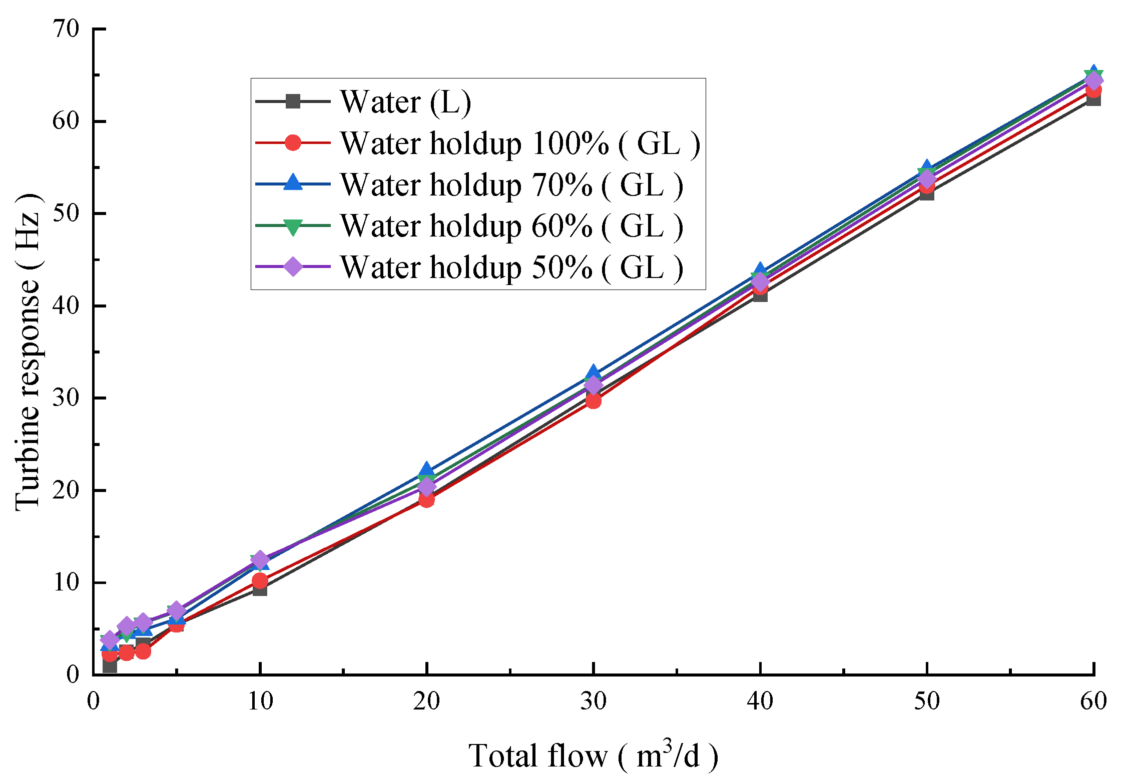
(3)

Experimental research on simulated wells has shown that when the gas phase flow is under 15 m³/d, the turbine’s response increases with the increase in the low flow of liquid. Moreover, the output results show that the DGLS can isolate the gas phase from the liquid phase. However, when the gas phase flow continues to increase, the turbine response reaches an inflection point at low liquid volume, and the DGLS’s gas–liquid separation effect is minimal.

Our research demonstrates that a DGLS is feasible in phase isolation when the medium is oil–gas–water multiphase flow. The DGLS design provides a theoretical basis for the actual production and has application guiding significance as well.

References

- Liu, X.B.; Hu, J.H.; Shan, F.J.; Cai, B.; Su, X.; Chen, Q. Conductance Sensor for Measurement of the Fluid Water cut and Flow rate in Production Wells. Chem. Eng. Commun. 2010, 197, 232–238. [Google Scholar] [CrossRef]
- Han, Y.L.; Wu, D.; Wang, J.G. Application of Horizontal Well Production Profile Logging Technology. Well Logging Technol. 2003, 27, 320–324. [Google Scholar]
- Wang, Z.Y.; Jin, N.D.; Gao, Z.K.; Zong, Y.; Wang, T. Nonlinear dynamical analysis of large diameter vertical upward oil–gas–water three-phase flow pattern characteristics. Chem. Eng. Sci. 2010, 65, 5226–5236. [Google Scholar] [CrossRef]
- Wang, Y.; Kong, L. The effect of consecutive bubbles on the response characteristics in electromagnetic flow meter. J. Comput. Inf. Syst. 2012, 8, 355–362. [Google Scholar]
- Zhai, L.S.; Bian, P.; Han, Y.F.; Gao, Z.-K.; Jin, N.-D. The measurement of gas–liquid two-phase flows in a small diameter pipe using a dual-sensor multi-electrode conductance probe. Meas. Sci. Technol. 2016, 27, 045101. [Google Scholar] [CrossRef]
- Hou, J.Y.; Li, Q.Q. Analysis of experimental characteristic of the bubbling umbrella. Pet. Instrum. 2007, 21, 57–59. [Google Scholar]
- Lebedev, Y.N.; Zil’berberg, I.A.; Lozhkin, Y.P.; Chekmenev, V.G. High efficiency mist eliminators. Chem. Technol. Fuels Oils 2002, 38, 42–45. [Google Scholar] [CrossRef]
- Shi, Y.H. Separation and pressure drop analysis for wire mesh demister. Petro-Chem. Equip. 2006, 5, 35–37. [Google Scholar]
- Al-Fulaij, H.; Cipollina, A.; Micale, G.; Ettouney, H.; Bogle, D. Eulerian-Eulerian modelling and computational fluid dynamics simulation of wire mesh demisters in MSF plant. Eng. Comput. 1984, 31, 1242–1261. [Google Scholar] [CrossRef]
- Da Fonseca Fadel, A.L. Oil-gas Separating Method and Bottom-Hole Spiral Separator with Gas Escape Channel. US Patent US6394182B1, 28 May 2002. [Google Scholar]
- Divonsir, L.; Robson De Oliveira, S.; Rogerio Floriao, S. Gas Separator with Automatic Level Control. US Patent US6554066B2, 19 April 2003. [Google Scholar]
- Wang, D.M.; Jiang, Y.L.; Wang, Y.; Liu, G.C.; Wang, B.; Wang, Z.P.; Han, Y.M. Gas-Liquid Separation Method and Multi-Settling Cup Gas Anchor. China Patent CN100532782C, 26 August 2009. [Google Scholar]
- Li, H.S. New labyrinth gas anchor and its application. China Pet. Mach. 1998, 26, 36–38. [Google Scholar]
- Liu, X.B.; Wang, Y.J.; Xie, R.H.; Zhang, Y.; Huang, C.; Li, L. Novel Four-Electrode Electromagnetic Flowmeter for the Measurement of Flow Rate in Polymer-Injection Wells. Chem. Eng. Commun. 2016, 203, 37–46. [Google Scholar] [CrossRef]
- Zhai, L.S.; Jin, N.D.; Zong, Y.B.; Wang, Z.; Gu, M. The development of a conductance method for measuring liquid holdup in horizontal oil-water two-phase flows. Meas. Sci. Technol. 2012, 23, 344–347. [Google Scholar] [CrossRef]
- Kong, W.H.; Kong, L.F.; Li, L.; Liu, X.B.; Cui, T. The influence on response of axial rotation of a six-group local-conductance probe in horizontal oil-water two-phase flow. Meas. Sci. Technol. 2017, 28, 065104. [Google Scholar]
- Yang, Y.Z.; Li, G.J.; Zhou, F.D. The Effect of Sudden Change in Pipe Diameter on Flow Patterns of Air-Water Two-Phase Flow in Vertical Pipe (I) Sudden-Contraction Cross-Section. Chin. J. Chem. Eng. 2001, 9, 116–119. [Google Scholar]
- Reynolds, O. An Experimental Investigation of the Circumstances Which Determine Whether the Motion of Water Shall Be Direct or Sinuous, and of the Law of Resistance in Parallel Channels. Proc. R. Soc. Lond. 1883, 35, 84–99. [Google Scholar]
- Debangshu Guha, P.; Ramachandran, A.; Dudukovic, M.P.; Derksen, J.J. Evaluation of large Eddy simulation and Euler-Euler CFD models for solids flow dynamics in a stirred tank reactor. AIChE J. 2008, 54, 766–778. [Google Scholar] [CrossRef]
- Benyahia, S.; Syamlal, M.; OBrien, T.J. Evaluation of boundary conditions used to model dilute, turbulent gas/solids flows in a pipe. Powder Technol. 2005, 156, 62–72. [Google Scholar] [CrossRef]