Article

Mathematical Analysis of Non-Isothermal Reaction–Diffusion Models Arising in Spherical Catalyst and Spherical Biocatalyst

by
Vivek Mani Tripathi
1,
Hari Mohan Srivastava
2,3,4,5,*,
Harendra Singh
6,
Chetan Swarup
7 and
Sudhanshu Aggarwal
8
1
Department of Engineering, Uttar Pradesh Textile Technology Institute, Kanpur 208001, India
2
Department of Mathematics and Statistics, University of Victoria, Victoria, BC V8W 3R4, Canada
3
Department of Medical Research, China Medical University Hospital, China Medical University, Taichung 40204, Taiwan
4
Department of Mathematics and Informatics, Azerbaijan University, 71 Jeyhun Hajibeyli Street, Baku AZ1007, Azerbaijan
5
Section of Mathematics, International Telematic University Uninettuno, I-00186 Rome, Italy
6
Department of Mathematics, Post-Graduate College, Ghazipur 233001, India
7
Department of Basic Science, College of Science and Theoretical Studies, Saudi Electronic University, Riyadh 13316, Saudi Arabia
8
Department of Mathematics, National Post-Graduate College, Gorakhpur 273402, India
*
Author to whom correspondence should be addressed.
Appl. Sci. 2021, 11(21), 10423; https://doi.org/10.3390/app112110423
Submission received: 19 August 2021 / Revised: 26 October 2021 / Accepted: 1 November 2021 / Published: 5 November 2021
(This article belongs to the Topic Dynamical Systems: Theory and Applications)

Abstract

:
The theory of dynamical systems and their widespread applications involve, for example, the Lane–Emden-type equations which are known to arise in initial- and boundary-value problems with singularity at the   time   t = 0 . The main objective of this paper is to make use of some mathematical analytic tools and techniques in order to numerically solve some reaction–diffusion equations, which arise in spherical catalysts and spherical biocatalysts, by applying the Chebyshev spectral collocation method. The proposed scheme has good accuracy. The results are demonstrated by means of illustrative graphs and numerical tables. The accuracy of the proposed method is verified by a comparison with the results which are derived by using analytical methods.

1. Introduction

The Lane–Emden-type equations are known to arise in initial- and boundary-value problems with singularity at the   time   t = 0 . Analytical solutions in the neighbourhood of t = 0 are always possible to find (see [1,2]), such as those given in [3,4,5,6]:
v ( t ) + γ t v ( t ) + g ( v ( t ) ) = 0 ,   0 t 1 , γ > 0
with the following boundary conditions:
v ( 0 ) = b 1   and   v ( 1 ) = b 2
Here, v ( t ) denotes the unknown function on [ 0 , 1 ] , v ( 0 ) denotes the derivative of v ( t ) at time t = 0 , and   b 1   a n d   b 2 are constants.
Equation (1) arises in astrophysics and many other branches of science such as physics, chemistry and bio-mathematics (see, for example, [7,8,9,10,11]).

1.1. Spherical Catalyst Model

The Lane–Emden boundary value problem (BVP) models the chemical species dimensionless concentration within a spherical catalyst and is given in [12] as follows:
v ( t ) + 2 t v ( t ) ρ 2 v ( t ) exp ( α μ ( 1 v ( t ) ) 1 + μ ( 1 v ( t ) ) ) = 0
with the following boundary conditions:
v ( 0 ) = 0   and   v ( 1 ) = 1
The effectiveness factor τ is defined by:
τ = 3 ρ 2 d v d t | t = 1

1.2. Mathematical Model of the Spherical Biocatalyst Equation

The chemical species dimensionless concentration within a spherical biocatalyst is modelled by the Lane–Emden equation and is written as follows (see [13]):
v ( t ) + 2 t v ( t ) ρ 2 ( 1 + μ ) v ( t ) 1 + μ v ( t ) = 0
together with following boundary conditions:
v ( 0 ) = 0   and   v ( 1 ) = 1
Here, in this article, we consider spherical catalytic and spherical biocatalyst pellets, in which non-isothermal single reactions take place.
In refs. [14,15], analytical techniques are used to solve these models. In the year 2017, Wazwaz [16] used a variational iteration method to solve these models. Subsequently, in the year 2018, the OHAM technique was used to solve these spherical models (see, for details, [17]). By using the third-order approximation, these models were solved numerically in [18]. Furthermore, in [14], these spherical models are solved by using a numerical technique.
Here, in our present investigation, we propose a spectral collocation method by using the shifted Chebyshev polynomials for finding the approximate solutions of the spherical catalyst and spherical biocatalyst models. In this method, we approximate the unknowns by using the shifted Chebyshev polynomials and truncate then to a finite dimension. Then, by the use of approximations, the spherical catalyst and spherical biocatalyst models are changed into a system of simpler equations whose solution leads to the approximate solution of the spherical catalyst and spherical biocatalyst models. The spectral collocation method has been used by many authors in order to analyse mathematical models, including fractional-order models, with applications in physical and engineering sciences and in many other fields (see [19,20,21,22,23,24,25,26,27,28,29,30,31,32,33,34,35,36,37,38]). Detailed applications of fractional calculus in science and engineering can be found in [39]. Some applications of iterative and spectral methods to solve real-world problems can be seen in [40,41,42,43]. The results, which we have found in this article, are demonstrated numerically and illustrated graphically. The main finding of this paper is that the proposed technique is easy for computation purposes and timesaving. The results will be helpful for researchers working on applied chemistry. We have performed all computations on the programming software MATLAB R2018b.

2. Preliminaries

The third-kind Chebyshev polynomials are defined by the following equivalent forms [44,45]:
V m ( t ) = cos ( m + 1 2 ) θ cos θ 2 = 2 2 m ( 2 m 2 ) P m ( 1 2 , 1 2 ) ( t )
where t = cos θ ,   θ [ 0 , π ] and P m ( α ,   β ) ( t ) is the Jacobi polynomial of degree m .
The equivalent analytical form of shifted Chebyshev polynomials of the third kind ( α = 1 2 ,   β = 1 2 ) is given by
V i ( t ) = k = 0 i ( 1 ) i k Γ ( i + 3 2 ) Γ ( i + k + 1 ) Γ ( k + 3 2 ) Γ ( i + 1 ) ( i k ) ! k ! t k
The shifted Chebyshev polynomials of the third kind are orthogonal in the interval [0, 1] with respect to the following weight function:
w ( t ) = t 1 t
and have their orthogonality property as follows:
0 1 V n ( t ) V m ( t ) w ( t ) d t = { π 2 ,             n = m 0 ,               n m
A function f L w ( t ) 2 [ 0 ,   1 ] , with | f ( t ) | Q , can be written as follows:
f ( t ) = lim n i = 0 n c i V i ( t ) ,
where
c i = f ( t ) , V i ( t ) = 2 π w 0 1 f ( t ) V i ( t ) w ( t ) d t
The finite-dimensional approximation for Equation (6) is given by
f i = 0 m c i V i ( t ) = C T λ m ( t ) ,
where
C = [ c 0 , c 1 , . , c m ] T and   λ m ( t ) = [ V 0 , V 1 , . , V m ] T
Theorem 1.
If λ m ( t ) = [ V 0 , V 1 , . , V m ] T denotes the shifted Chebyshev vector and if v > 0 , then:
I v V i ( t ) = I ( v ) λ m ( t ) ,
where I ( v ) = ( ε ( i , j ) )   is the ( m + 1 ) × ( m + 1 ) operational matrix of integral of order v and its ( i , j ) th entry is given by
ε ( i , j ) = k = 0 i l = 0 j ( 1 ) i + j k l Γ ( 1 2 ) Γ ( i + 3 2 ) Γ ( i + k + 1 ) Γ ( j + l + 1 ) Γ ( v + k + l + 3 2 ) ( 2 j + 1 ) j ! ( i k ) ! ( j l ) ! ( l ) !   Γ ( k + 3 2 ) Γ ( i + 1 ) Γ ( v + k + 1 ) Γ ( j + 1 2 ) Γ ( l + 3 2 ) Γ ( k + l + v + 2 ) .
Proof. 
Please see [28].
In this paper, we will use this matrix for v = 1 ,   2 . □

3. Outline of the Proposed and Used Method

In this section, we give an outline of our proposed method. Models with undetermined constants as an intermediate step in the determination of the non-linear BVP are written as follows:
v ( t ) + 2 t v ( t ) ρ 2 v ( t ) exp ( α μ ( 1 v ( t ) ) 1 + μ ( 1 v ( t ) ) ) = 0
v ( t ) + 2 t v ( t ) ρ 2 ( 1 + μ ) v ( t ) 1 + μ v ( t ) = 0
with
v ( 0 ) = β ,     v ( 0 ) = 0   and   v ( 1 ) = 1
where v ( 0 ) = β represents an undetermined constant.
We first choose the following approximation:
v ( t ) = C T λ n ( t )
Then, by the first-order integration of Equation (18), we obtain
v ( t ) = C T I ( 1 ) λ n ( t ) + P T λ n ( t )
Taking the first-order integration of Equation (19), we find that
v ( t ) = C T I ( 2 ) λ n ( t ) + P T I ( 1 ) λ n ( t ) + Q T λ n ( t )
where
v ( 0 ) = P T λ n ( t )   and   v ( 0 ) = Q T λ n ( t )
We now take
1 = D T λ n ( t )

3.1. The Spherical Catalyst Equation

Combining Equations (15) and (17)–(22), we obtain
C T λ n ( t ) + 2 t ( C T I ( 1 ) + P T ) λ n ( t ) ρ 2 ( C T I ( 2 ) + P T I ( 1 ) + Q T ) λ n ( t ) exp ( α μ ( D T ( C T I ( 2 ) + P T I ( 1 ) + Q T ) ) λ n ( t ) ( D T + μ ( D T ( C T I ( 2 ) + P T I ( 1 ) + Q T ) ) ) λ n ( t ) ) = 0
For Equation (23), the residual is defined by
R n ( t ) = C T λ n ( t ) + 2 t ( C T I ( 1 ) + P T ) λ n ( t ) ρ 2 ( C T I ( 2 ) + P T I ( 1 ) + Q T ) λ n ( t ) exp ( α μ ( D T ( C T I ( 2 ) + P T I ( 1 ) + Q T ) ) λ n ( t ) ( D T + μ ( D T ( C T I ( 2 ) + P T I ( 1 ) + Q T ) ) ) λ n ( t ) )
Collocating Equation (24) at n 1 points, which are given by
t i = i n ,       i = 1 , 2 , , n 1
we have
R n ( t i ) = C T λ n ( t i ) + 2 t i ( C T I ( 1 ) + P T ) λ n ( t i ) ρ 2 ( C T I ( 2 ) + P T I ( 1 ) + Q T ) λ n ( t i ) exp ( α μ ( D T ( C T I ( 2 ) + P T I ( 1 ) + Q T ) ) λ n ( t i ) ( D T + μ ( D T ( C T I ( 2 ) + P T I ( 1 ) + Q T ) ) ) λ n ( t i ) )
The corresponding initial and boundary conditions can be written as follows:
( C T I ( 2 ) + P T I ( 1 ) + Q T ) λ n ( 0 ) = β ( C T I ( 2 ) + P T I ( 1 ) + Q T ) λ n ( 1 ) = 1
From Equations (25)–(27), we obtain a system of n + 1 equations. Solving this system, we obtain our solution for the spherical catalyst model.

3.2. The Spherical Biocatalyst Equation

Combining Equations (16)–(22), we obtain
C T λ n ( t ) + 2 t ( C T I ( 1 ) + P T ) λ n ( t ) ρ 2 ( 1 + μ ) ( C T I ( 2 ) + P T I ( 1 ) + Q T ) λ n ( t ) ( D T + μ ( C T I ( 2 ) + P T I ( 1 ) + Q T ) ) λ n ( t ) = 0
For Equation (28), the residual is defined by
R n ( t ) = C T λ n ( t ) + 2 t ( C T I ( 1 ) + P T ) λ n ( t ) ρ 2 ( 1 + μ ) ( C T I ( 2 ) + P T I ( 1 ) + Q T ) λ n ( t ) ( D T + μ ( C T I ( 2 ) + P T I ( 1 ) + Q T ) ) λ n ( t )
Collocating Equation (28) at n 1 points which are given by
t i = i n ,       i = 1 , 2 , , n 1
we find that
R n ( t i ) = C T λ n ( t i ) + 2 t i ( C T I ( 1 ) + P T ) λ n ( t i ) ρ 2 ( 1 + μ ) ( C T I ( 2 ) + P T I ( 1 ) + Q T ) λ n ( t i ) ( D T + μ ( C T I ( 2 ) + P T I ( 1 ) + Q T ) ) λ n ( t i )
The corresponding initial and boundary conditions can be written as follows:
( C T I ( 2 ) + P T I ( 1 ) + Q T ) λ n ( 0 ) = β
( ( C T I ( 2 ) + P T I ( 1 ) + Q T ) λ n ( 1 ) = 1
From Equations (30)–(32), we obtain a system of n + 1 equations. Solving this system, we obtain our solution for the spherical biocatalyst model.

4. Convergence Analysis

Theorem 2.
Let d 2 v ( t ) d t 2 L w ( t ) 2 [ 0 , 1 ] and ( d 2 v ( t ) d t 2 ) n be the n t h approximation of it obtained by ( n + 1 ) shifted Chebyshev polynomials of the third kind. Additionally, let | d 4 v ( t ) d t 4 | < M for a positive constant M.Then, as n , the approximated value ( d 2 v ( t ) d t 2 ) n converges to the exact value d 2 v ( t ) d t 2 with the following inequality for the expansion coefficients of d 2 v ( t ) d t 2 :
| c n | < M n 2
Proof. 
Let
d 2 v ( t ) d t 2 = i = 1 c i V i ( t )
Taking the n t h approximation of the above equation, we obtain
( d 2 v ( t ) d t 2 ) n = i = 1 n c i V i ( t )
By subtracting Equation (35) from Equation (34), we find that
( d 2 v ( t ) d t 2 ) ( d 2 v ( t ) d t 2 ) n = i = n + 1 c i V i ( t )
The coefficients in Equation (36) are given by
c n = 2 π 0 1 ( d 2 v ( t ) d t 2 ) V n ( t ) w ( t ) d t c n = 2 π 0 1 ( d 2 v ( t ) d t 2 ) V n ( t ) t 1 t d t
If we set 2 t 1 = cos y , then we have
c n = 2 π 0 π ( d 2 v d y 2 ( 1 + cos y 2 ) ) cos ( y + 1 2 ) y cos ( y 2 ) d y
Integrating Equation (38), we obtain
c n = 1 4 π 0 π ( d 4 v d y 4 ( 1 + cos y 2 ) ) ξ n ( y ) d y
where ξ n ( y ) = sin y [ 1 n ( sin ( n 1 ) y n 1 sin ( n + 1 ) y n + 1 ) + 1 n + 1 ( sin n y n sin ( n + 2 ) y n + 2 ) ] .
We now observe that
| ξ n ( y ) | = | sin y [ 1 n ( sin ( n 1 ) y n 1 sin ( n + 1 ) y n + 1 ) + 1 n + 1 ( sin n y n sin ( n + 2 ) y n + 2 ) ] | = | [ 1 n ( 1 n 1 1 n + 1 ) + 1 n + 1 ( 1 n 1 n + 2 ) ] | | [ 1 n ( 1 n 1 + 1 n + 1 ) + 1 n + 1 ( 1 n + 1 n + 2 ) ] | < 1 n 2
Furthermore, from Equation (40), we can write
| c n | = | 1 4 π 0 π ( d 4 x d y 4 ( 1 + cos y 2 ) ) ξ n ( y ) d y |
Thus, from the given condition, we obtain
| c n | F 4 π 0 π | ξ n ( y ) | d y
which, in view of Equation (40), yields
| c n | < M π n 2 0 π d y
that is,
| c n | < M n 2
for a given positive constant M.
So, in Equation (36), if we proceed to the limit as   n , we obtain
( d 2 v ( t ) d t 2 ) n d 2 v ( t ) d t 2

5. Error Estimation

Theorem 3.
Let d 2 v ( t ) d t 2 L w ( t ) 2 [ 0 , 1 ] and ( d 2 v ( t ) d t 2 ) n be the n t h approximation of it obtained by ( n + 1 ) shifted Chebyshev polynomials of the third kind. If | d 4 v ( t ) d t 4 | < M for some positive constant M, then the following error estimate holds true:
E n ,     d 2 v ( t ) d t 2 2 π M 2 12 G 3 ( n + 1 )
where
E n ,     d 2 v ( t ) d t 2 = ( 0 1 | ( d 2 v ( t ) d t 2 ) ( d 2 v ( t ) d t 2 ) n | 2 w ( t ) d t ) 1 2
and G n ( y ) is a Poly-Gamma function given by
G n ( y ) = ( 1 ) n + 1 n ! j = 0 1 ( y + j ) n + 1
Proof. 
The error term is given by
E n ,     d 2 v ( t ) d t 2 = ( 0 1 | ( d 2 v ( t ) d t 2 ) ( d 2 v ( t ) d t 2 ) n | 2 w ( t ) d t ) 1 2 = ( 0 1 | i = n + 1 c i V i ( t ) | 2 w ( t ) d t ) 1 2
By using the orthogonality property of the third-kind Chebyshev polynomials in Equation (43), we obtain
E n ,     d 2 v ( t ) d t 2 = ( π 2 i = n + 1 | c i | 2 ) 1 2
and
E n ,     d 2 v ( t ) d t 2 2 π P 2 2 i = n + 1 1 i 4 ,                  
where
| d 4 v ( t ) d t 4 | < M
for some positive constant M.
Since
i = n + 1 1 i 4 = 1 6 G 3 ( n + 1 )
we find from Equations (32) and (33) that
E n ,     d 2 v ( t ) d t 2 2 π M 2 12 G 3 ( n + 1 )

6. Numerical Simulations and Discussion

In this section, numerical simulations of our results are presented by using illustrative figures and numerical tables. We show the effect of the parameters μ ,   α and ρ on the concentration of the substance.

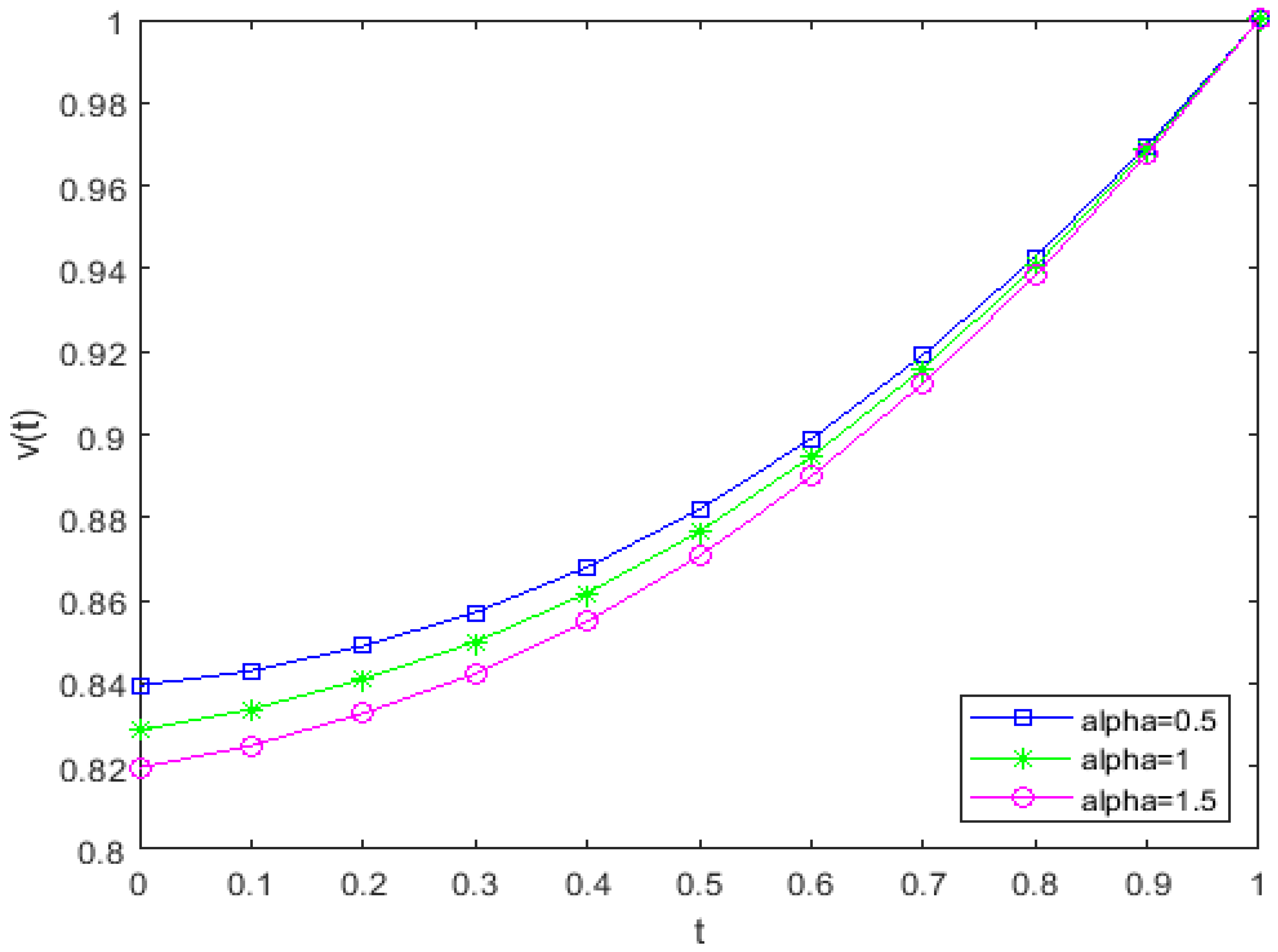
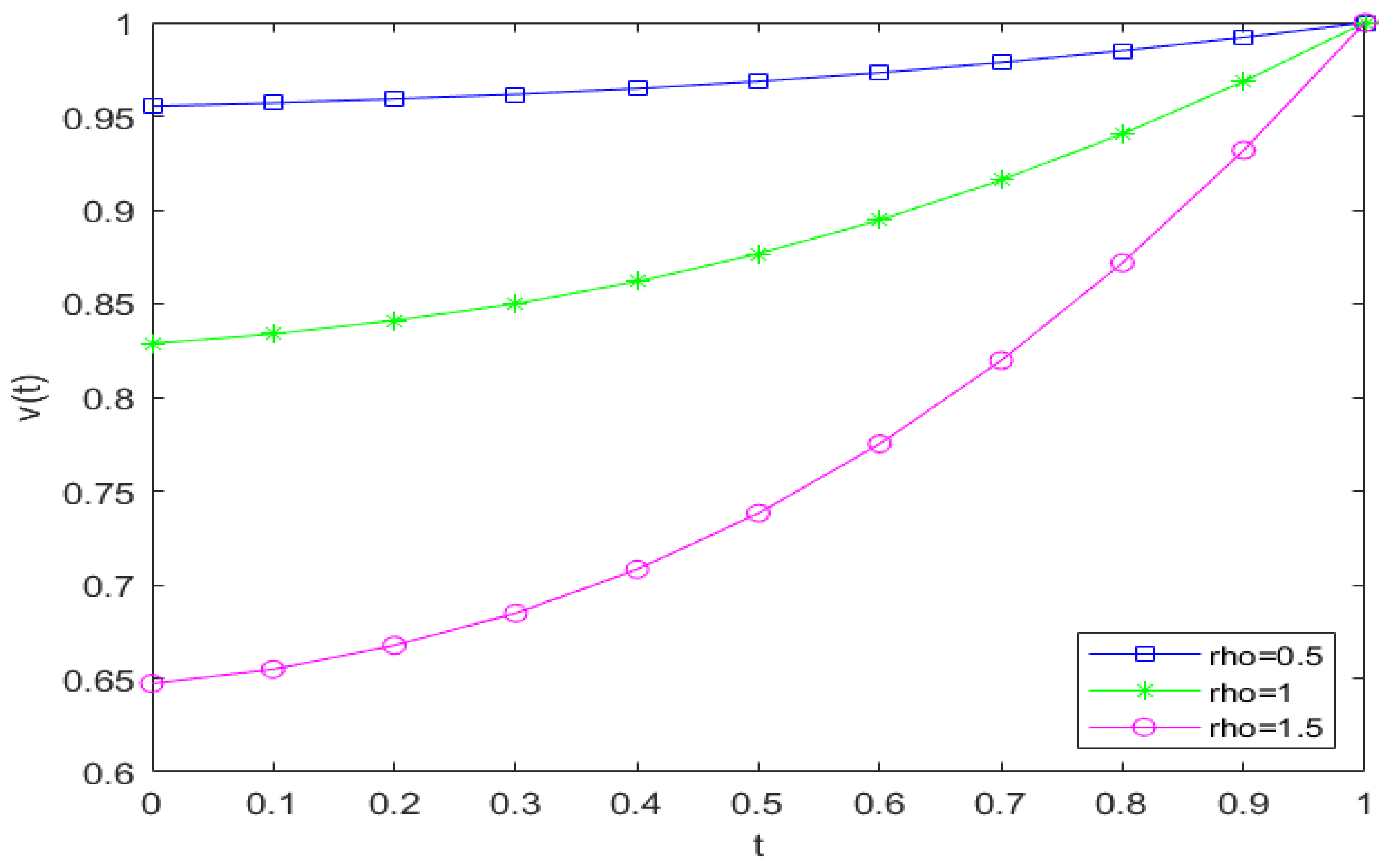
6.1. Results for the Spherical Catalyst Model

We first show the effect of the parameters μ ,   α and ρ on the concentration of the substance in a spherical catalyst model. Figure 1 illustrates the behaviour of the concentration v(t; α, μ, ρ) of the substance for different values of α at μ = 1 and ρ = 1 .
Figure 2 illustrates the behaviour of the concentration v ( t ;   α , μ , ρ ) of the substance for different values of ρ at μ = 1 and α = 1 . From Figure 1 and Figure 2, we can see that the concentration of the substance shows a continuous behaviour with the values of the parameters α and ρ .
In Table 1, the results are compared between those derived here by the proposed method and by the method which was used in [16] for different choices of   α and μ = 1 and ρ = 1 .
In Table 2 below, the results are compared between those derived here by our proposed method and by the method used in [16] for different choices of   ρ and μ = 1 and α = 1 .
In Table 3 below, the effectiveness factor ( τ ) for different choices of the parameters are listed. From Table 3, we can see that τ increases with the increase in α and decreases with the increase in ρ .
In Table 4, we have listed CPU time of computations for different dimensions of basis.

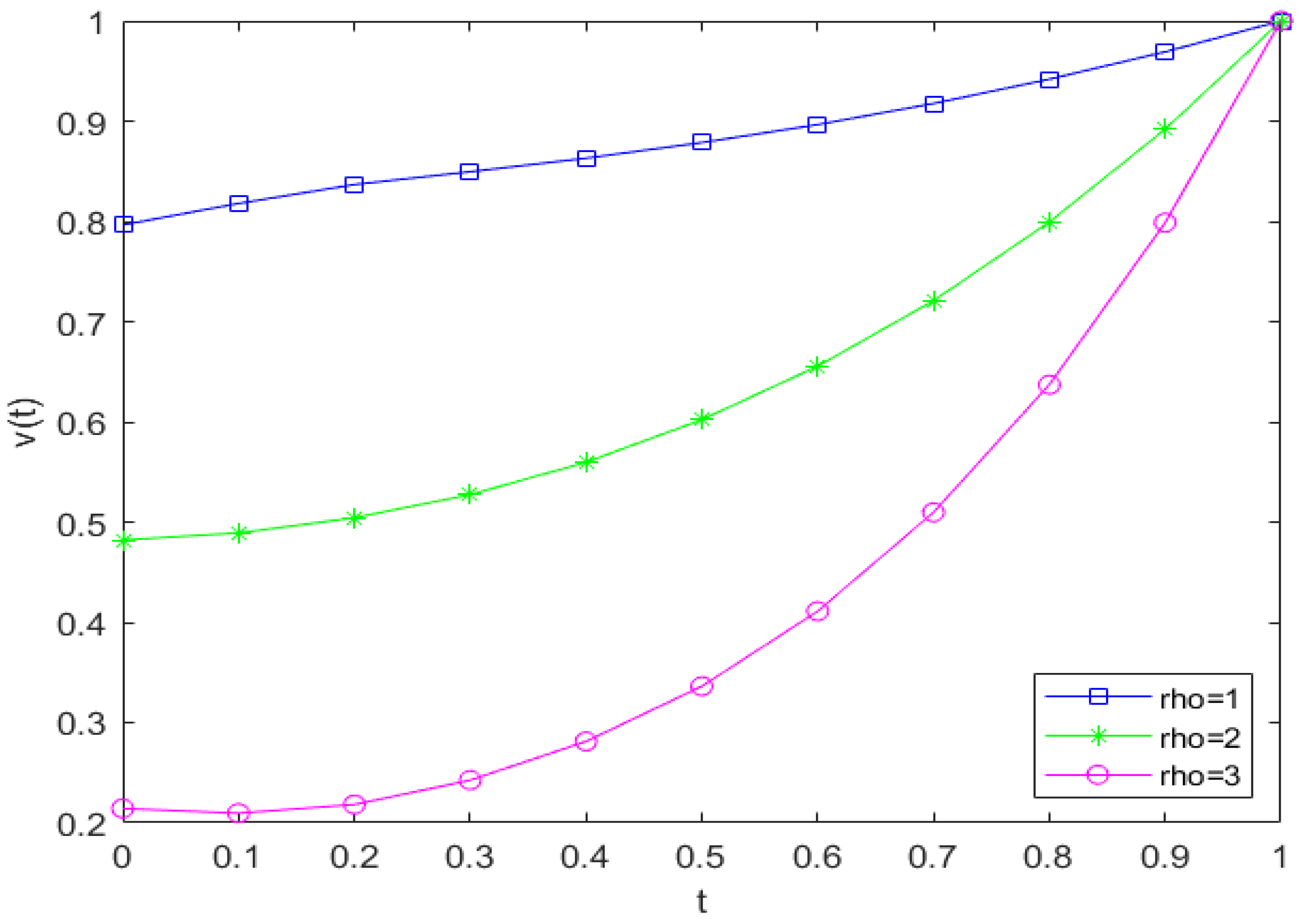
6.2. Results for the Spherical Biocatalyst Model

We show here the effect of the parameters μ ,   α and ρ on the concentration of the substance in a spherical biocatalyst model. Figure 1 shows the behaviour of the concentration v ( t ;   α , μ , ρ ) of the substance for different values of ρ at μ = 2 . From Figure 3, we can see that the concentration of the substance shows a continuous behaviour with the values of ρ .
In Table 5 below, the results are compared between those derived here by the proposed method and those by the method used in [16] for different choices of ρ and μ = 2 .
In Table 6, the τ values for different choices of parameters are listed. From Table 6, we can see that τ decreases with the increase in  ρ .

7. Conclusions

In this article, we have studied the behaviour of the concentration of the pellets at the spherical origin t = 0 . The main advantages of the technique, which we have proposed and used here, are that it handles the singularity at the origin remarkably easily and it provides an accurate solution at the origin and in the neighbourhood of the origin. Our proposed method is easy to handle because both of the mathematical models, which we have considered in this article, are converted into a system of non-linear algebraic equations. From the illustrative figures and numerical tables, the accuracy and efficiency of the proposed method are sufficiently clear. It is also observed that the desired accuracy is achieved by using a lower number of the basis elements. In our future communications, we can use a different class of polynomials and wavelets in order to possibly achieve a better accuracy.

Author Contributions

All authors have equal contributions. All authors have read and agreed to the published version of the manuscript.

Funding

This research received no external funding.

Institutional Review Board Statement

Not Applicable.

Informed Consent Statement

Not Applicable.

Data Availability Statement

Not Applicable.

Conflicts of Interest

The authors declare no conflict of interest.

Notations and Abbreviations

C A Concentration inside the pellet
C A s Concentration at the surface of pellet
D Effective diffusivity
E Activation energy
Δ H Heat of reaction
K Inside effective thermal conductivity
K r e f Reference reaction constant
r Radial distance
R g Universal gas constant
r A Arrhenius reaction rate
R Spherical catalytic pellet radius
T s Temperature at the surface
T Temperature inside the pellet.
v Radial-direction dimensionless concentration
t Dimensionless distance
α Dimensionless heat of reaction
μ Dimensionless activation energy
τ Effectiveness factor
ρ Thiele modulus

References

  1. Davis, H.T. Introduction to No nlinear Differential and Integral Equations; Dover Publications: New York, NY, USA, 1962. [Google Scholar]
  2. Lane, J.H. On theoretical temperature of the sun under the hypothesis of a gaseous mass maintaining its internal heat and depending on the laws of gases known to terrestrial experiment. Am. J. Sci. Arts 1870, 50, 57–74. [Google Scholar] [CrossRef]
  3. Van Gorder, R.A. Exact first integrals for a Lane–Emden equation of the second kind modeling a thermal explosion in a rectangular slab. New Astron. 2011, 16, 492–497. [Google Scholar] [CrossRef]
  4. Singh, H. An efficient computational method for the approximate solution of nonlinear Lane-Emden type equations arising in astrophysics. Astrophys. Space Sci. 2018, 363, 363–371. [Google Scholar] [CrossRef]
  5. Rach, R.; Duan, J.-S.; Wazwaz, A.-M. On the Solution of Non-Isothermal Reaction-Diffusion Model Equations in a Spherical Catalyst by the Modified Adomian Method. Chem. Eng. Commun. 2015, 202, 1081–1088. [Google Scholar] [CrossRef]
  6. Singh, H.; Srivastava, H.M.; Kumar, D. A reliable algorithm for the approximate solution of the nonlinear Lane-Emden type equations arising in astrophysics. Numer. Methods Partial Differ. Equ. 2014, 34, 1524–1555. [Google Scholar] [CrossRef]
  7. Chandrasekhar, S. Introduction to the Study of Stellar Structure; Dover Publications: New York, NY, USA, 1967. [Google Scholar]
  8. Horedt, G.M. Polytropes: Applications in Astrophysics and Related Fields; Kluwer Academic Publishers: Dordrecht, The Netherlands, 2004. [Google Scholar]
  9. Duan, J.-S.; Rach, R.; Wazwaz, A.M. Steady-state concentrations of carbon dioxide absorbed into phenylglycidyl ether solutions by the Adomian decomposition method. J. Math. Chem. 2015, 53, 1054–1067. [Google Scholar] [CrossRef]
  10. Wazwaz, A.M. The variational iteration method for solving new fourth-order Emden–Fowler type equations. Chem. Eng. Commun. 2015, 202, 1425–1437. [Google Scholar] [CrossRef]
  11. Wazwaz, A.M. Solving systems of fourth-order Emden–Fowler type equations by the variational iteration method. Chem. Eng. Commun. 2016, 203, 1081–1092. [Google Scholar] [CrossRef]
  12. Rach, R.; Duan, J.-S.; Wazwaz, A.M. Solving coupled Lane–Emden boundary value problems in catalytic diffusion reactions by the Adomian decomposition method. J. Math. Chem. 2014, 52, 255–267. [Google Scholar] [CrossRef]
  13. Saadatmandi, A.; Nafar, N.; Toufighi, S.P. Numerical study on the reaction cum diffusion process in a spherical biocatalyst. Iran. J. Math. Chem. 2014, 5, 47–61. [Google Scholar]
  14. Sevukaperumal, S.; Rajendran, L. Analytical solution of the concentration of species using modified Adomian decomposition method. Int. J. Math. Arch. 2013, 4, 107–117. [Google Scholar]
  15. Danish, M.; Kumar, S.; Kumar, S. OHAM solution of a singular BVP of reaction cum diffusion in a biocatalyst. Int. J. Appl. Math. 2011, 41, 223–227. [Google Scholar]
  16. Wazwaz, A.M. Solving the non-isothermal reaction-diffusion model equations in a spherical catalyst by the variational iteration method. Chem. Phys. Lett. 2017, 679, 132–136. [Google Scholar] [CrossRef]
  17. Singh, R. Optimal homotopy analysis method for the non-isothermal reaction–diffusion model equations in a spherical catalyst. J. Math. Chem. 2018, 56, 2579–2590. [Google Scholar] [CrossRef]
  18. Li, X.-M.; Chen, X.-D.; Chen, N.-X. A third-order approximate solution of the reaction diffusion process in an immobilized biocatalyst particle. Biochem. Eng. J. 2014, 17, 65–69. [Google Scholar] [CrossRef]
  19. Singh, H. A new numerical algorithm for fractional model of Bloch equation in nuclear magnetic resonance. Alex. Eng. J. 2016, 55, 2863–2869. [Google Scholar] [CrossRef] [Green Version]
  20. Singh, H. Operational matrix approach for approximate solution of fractional model of Bloch equation. J. King Saud Univ. Sci. 2017, 29, 235–240. [Google Scholar] [CrossRef]
  21. Petráš, I. Modeling and numerical analysis of fractional-order Bloch equations. Comput. Math. Appl. 2011, 61, 341–356. [Google Scholar] [CrossRef]
  22. Ahmadian, A.; Chan, C.S.; Salahshour, S.; Vaitheeswaran, V. FTFBE: A numerical approximation for fuzzy time-fractional Bloch equation. In Proceedings of the International Conference on Fuzzy systems (FUZZ-IEEE), World Congress on Computational Intelligence, Beijing, China, 6–11 July 2014; IEEE: Piscataway, NJ, USA, 2014; pp. 418–423. [Google Scholar]
  23. Wu, J.-L. A wavelet operational method for solving fractional partial differential equations numerically. Appl. Math. Comput. 2009, 214, 31–40. [Google Scholar] [CrossRef]
  24. Singh, H.; Srivastava, H.M.; Kumar, D. A reliable numerical algorithm for the fractional vibration equation. Chaos Solitons Fractals 2017, 103, 131–138. [Google Scholar] [CrossRef]
  25. Tohidi, E.; Bhrawy, A.H.; Erfani, K. A collocation method based on Bernoulli operational matrix for numerical solution of generalized pantograph equation. Appl. Math. Model. 2013, 37, 4283–4294. [Google Scholar] [CrossRef]
  26. Kazem, S.; Abbasbandy, S.; Kumar, S. Fractional-order Legendre functions for solving fractional-order differential equations. Appl. Math. Model. 2013, 37, 5498–5510. [Google Scholar] [CrossRef]
  27. Singh, C.S.; Singh, H.; Singh, V.K.; Singh, O.P. Fractional order operational matrix methods for fractional singular integro-differential equation. Appl. Math. Model. 2016, 40, 10705–10718. [Google Scholar] [CrossRef]
  28. Singh, H.; Srivastava, H.M. Jacobi collocation method for the approximate solution of some fractional-order Riccati differential equations with variable coefficients. Phys. A Stat. Mech. Appl. 2019, 523, 1130–1149. [Google Scholar] [CrossRef]
  29. Singh, C.S.; Singh, H.; Singh, S.; Kumar, D. An efficient computational method for solving system of nonlinear generalized Abel integral equations arising in astrophysics. Phys. A Stat. Mech. Appl. 2019, 525, 1440–1448. [Google Scholar] [CrossRef]
  30. Singh, H.; Pandey, R.K.; Baleanu, D. Stable numerical approach for fractional delay differential equations. Few-Body Syst. 2017, 58, 1–18. [Google Scholar] [CrossRef]
  31. Singh, H.; Singh, C.S. Stable numerical solutions of fractional partial differential equations using Legendre scaling functions operational matrix. Ain Shams Eng. J. 2018, 9, 717–725. [Google Scholar] [CrossRef]
  32. Podlubny, I. Fractional Differential Equations: An Introduction to Fractional Derivatives, Fractional Differential Equations, to Methods of Their Solution and Some of Their Applications; Mathematics in Science and Engineering; Academic Press: San Diego, CA, USA; London, UK, 1999; Volume 198. [Google Scholar]
  33. Cattani, C.; Srivastava, H.M.; Yang, X.-J. Fractional Dynamics; Emerging Science Publishers: Berlin, Germany, 2015. [Google Scholar]
  34. Singh, H.; Srivastava, H.M.; Hammouch, Z.; Nisar, K.S. Numerical simulation and stability analysis for the fractional-order dynamics of COVID-19. Results Phys. 2021, 20, 1–8. [Google Scholar] [CrossRef]
  35. Kilbas, A.A.; Srivastava, H.M.; Trujillo, J.J. Theory and Applications of Fractional Differential Equations; North-Holland Mathematical Studies; Elsevier (North-Holland) Science Publishers: Amsterdam, The Netherlands, 2006; Volume 204. [Google Scholar]
  36. Srivastava, H.M. Fractional-order derivatives and integrals: Introductory overview and recent developments. Kyungpook Math. J. 2020, 60, 73–116. [Google Scholar]
  37. Srivastava, H.M. Some parametric and argument variations of the operators of fractional calculus and related special functions and integral transformations. J. Nonlinear Convex Anal. 2021, 22, 1501–1520. [Google Scholar]
  38. Srivastava, H.M. An introductory overview of fractional-calculus operators based upon the Fox-Wright and related higher transcendental functions. J. Adv. Eng. Comput. 2021, 5, 135–166. [Google Scholar]
  39. Povstenko, Y. Linear Fractional Diffusion-Wave Equation for Scientists and Engineers; Birkhäuser: New York, NY, USA, 2015. [Google Scholar]
  40. Heydari, M.; Hosseini, S.M.; Loghmani, G.B. Numerical solution of singular IVPs of Lane-Emden type using integral operator and radial basis functions. Int. J. Ind. Math. 2011, 4, 135–146. [Google Scholar]
  41. Nikooeinejad, Z.; Heydari, M. Nash equilibrium approximation of some class of stochastic differential games: A combined Chebyshev spectral collocation method with policy iteration. J. Comput. Appl. Math. 2019, 362, 41–54. [Google Scholar] [CrossRef]
  42. Nikooeinejad, Z.; Delavarkhalafi, A.; Heydari, M. Application of shifted Jacobi pseudo spectral method for solving (in) finite-horizon min -max optimal control problems with uncertainty. Int. J. Control 2018, 91, 725–739. [Google Scholar] [CrossRef]
  43. Heydari, M.; Loghmani, G.B.; Hosseini, S.M.; Yildirim, A. A novel hybrid spectral-variational iteration method (H-S-VIM) for solving nonlinear equations arising in heat transfer. Iran. J. Sci. Technol. Trans. A 2013, 37, 501512. [Google Scholar]
  44. Mason, J.C.; Handscomb, D.C. Chebyshev Polynomials; Chapman and Hall/CRC: Boca Raton, FL, USA, 2003. [Google Scholar]
  45. Doman, B.G.S. The Classical Orthogonal Polynomials; World Scientific: Singapore, 2016. [Google Scholar]
Figure 1. Behaviour of the concentration at different values of the parameter.
Applsci 11 10423 g001
Figure 2. Effect of the Thiele modulus for different values of ρ on the concentration v ( t ;   α , μ , ρ ) .
Applsci 11 10423 g002
Figure 3. Effect of the Thiele modulus for different values of the parameter ρ on the concentration v ( t ;   μ , ρ ) .
Applsci 11 10423 g003
Table 1. Comparison of the results with different values of the parameter α .
t Present Method ( α = 0.5 ) Method in
[16]   ( α = 0.5 )
Present Method ( α = 1 ) Method in
[16]   ( α = 1 )
Present Method ( α = 1.5 ) Method in
[16]   ( α = 1.5 )
0.00.83946 0.83946 0.82874 0.828740.81965 0.81965
0.10.84301 0.84100 0.83376 0.83040 0.82499 0.82143
0.20.84901 0.84562 0.84102 0.83539 0.83276 0.82676
0.30.85710 0.85336 0.84995 0.84372 0.84231 0.83565
0.40.868010.86425 0.86171 0.85542 0.85487 0.84813
0.50.88193 0.87834 0.87656 0.87055 0.87069 0.86421
0.60.89893 0.89572 0.89458 0.88916 0.88980 0.88393
0.70.91917 0.91646 0.91591 0.91132 0.91234 0.90732
0.80.94270 0.94067 0.94058 0.93711 0.93825 0.93443
0.90.96960 0.96847 0.96858 0.96663 0.96747 0.96530
1.01.00000 1.00000 1.00000 1.00000 1.00000 1.00000
Table 2. Comparison of the results with different values of the parameter ρ .
t Present Method ( ρ = 0.5 ) Method in
[16]   ( ρ = 0.5 )
Present Method ( ρ = 1.5 ) Method in
[16]   ( ρ = 1.5 )
0.00.95541 0.95541 0.64719 0.64719
0.10.95708 0.95586 0.65480 0.65039
0.20.95924 0.95719 0.66754 0.66003
0.30.96164 0.95940 0.68476 0.67623
0.40.96473 0.96251 0.70812 0.69918
0.50.96858 0.96651 0.73814 0.72918
0.60.97322 0.97141 0.77515 0.76657
0.70.97868 0.97720 0.81960 0.81179
0.80.98496 0.98389 0.87175 0.86535
0.90.99206 0.99149 0.93181 0.92786
1.01.00000 1.00000 1.00000 1.00000
Table 3. Comparison of the effectiveness factor τ with different choices of the parameters.
β α ρ μ Present MethodMethod in [16]
0.8394623 0.5 110.9656645 1.003207
0.8287498 1.0 1 11 00.9943650 1.059701
0.81965801.5 111.0253210 1.098859
0.955417010.5 11.0041781 1.075815
0.828749811.0 10.9943650 1.059701
0.6471921 11.510.9637729 1.029147
Table 4. CPU time taken in computation for different values of n at β = 0.9554170509 , α = 1 ,   μ = 1 and ρ = 0.5 .
n Time (s)
48.201
718.034
1060.819
Table 5. Comparison of the results with different choices of the parameter ρ .
t Present Method ( ρ = 1 ) Method in
[16]   ( ρ = 1 )
Present Method ( ρ = 2 ) Method in
[16]   ( ρ = 2 )
Present Method ( ρ = 3 ) Method in
[16]   ( ρ = 3 )
0.00.79644 0.79644 0.48206 0.48206 0.21426 0.21426
0.10.83673 0.80322 0.50437 0.49965 0.21819 0.23594
0.20.863670.803220.504370.499650.218190.23594
0.30.84955 0.81262 0.52743 0.52202 0.24253 0.26447
0.40.86303 0.82544 0.55976 0.55404 0.28121 0.30696
0.50.87859 0.84227 0.60219 0.59640 0.33626 0.36575
0.60.89653 0.86338 0.65556 0.64999 0.41109 0.44360
0.70.91761 0.88914 0.72092 0.71586 0.50969 0.54338
0.80.94184 0.92005 0.79932 0.79522 0.63704 0.66792
0.90.96914 0.95674 0.89191 0.88944 0.79866 0.81958
1.01.00000 1.00000 1.00000 1.00000 1.00000 1.00000
Table 6. Comparison of the effectiveness factor τ with different choices of the parameters.
β ρ μ Present MethodMethod in [16]
0.7964472 110.9848465 1.4057760
0.4820697 210.9468011 0.8943578
0.2142606 310.7432604 0.6501860
Publisher’s Note: MDPI stays neutral with regard to jurisdictional claims in published maps and institutional affiliations.

