
MovieDIRec: Drafted-Input-Based Recommendation System for Movies


Abstract
:1. Introduction
- It is the subject of training and is input data that are continuously updated through learning once they are created ≈ preliminary and updatable object.
- These are the input data selected to describe the target in terms of the goal of the model ≈ select for a certain purpose.
- Verify the effect of Drafted-Input of movie/user on training and recommendation accuracy;
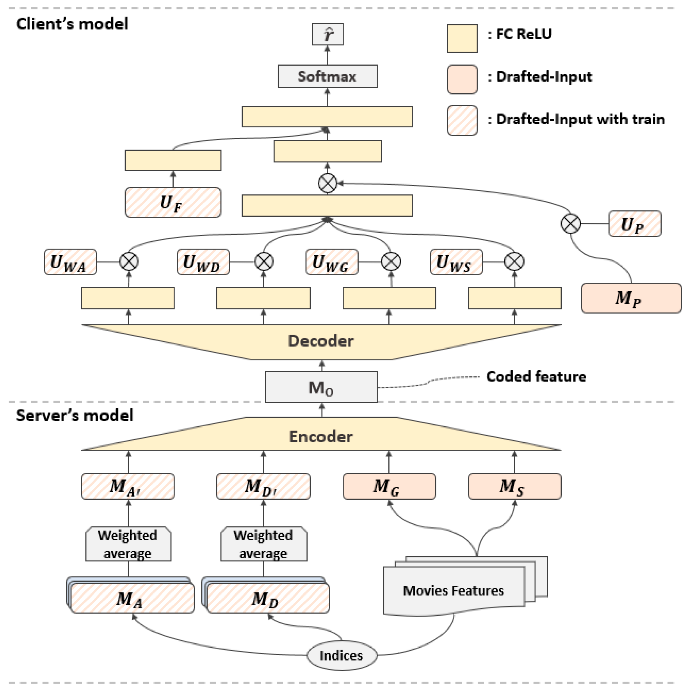
- Propose an inference resource distribution method based on Auto-Encoder considering the client–server environment;
- Propose a method to personalize by paying attention to specific preference features of items in the network using User’s weights extracted through a specific method.
2. Related Works
2.1. DNN-Based Recommendation System
2.2. TF-IDF
2.3. Truncated-SVD
2.4. Auto Encoder
3. Our Approach
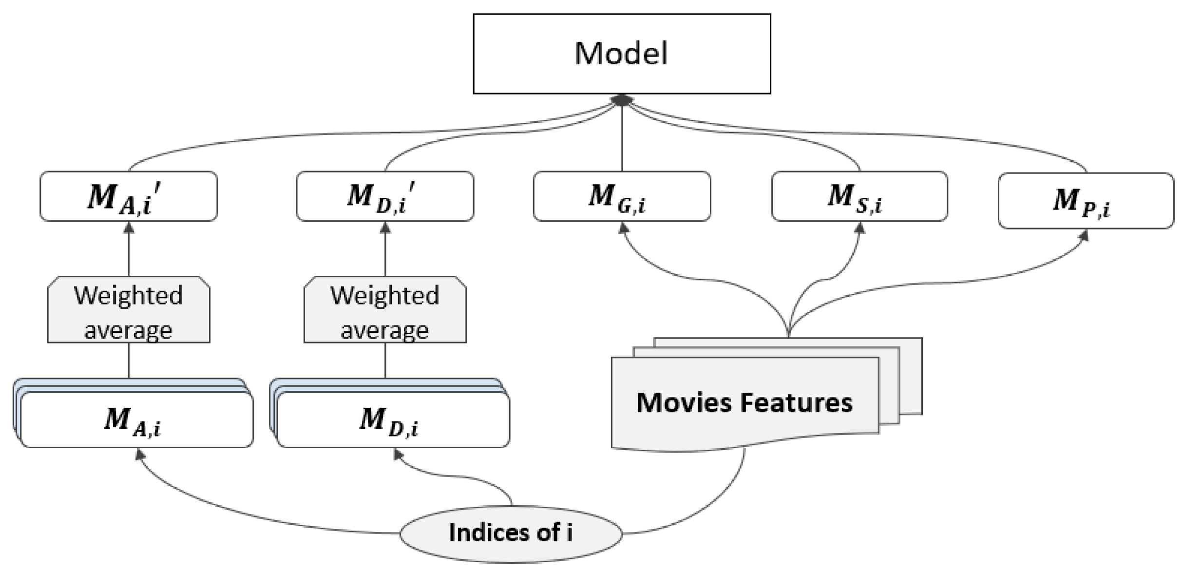
3.1. Drafted-Input
3.1.1. Movie Features
- Remove numbers and symbols that are not related to the story;
- Remove person names and attach NER(Named Entity Recognition) tags using the pre-trained Bert model [21];
- Remove movies with five or fewer descriptive words;
- Only words included in the movie plot were left, and TF-IDF was conducted only for words that appeared three or more times in all movies.
3.1.2. User Features
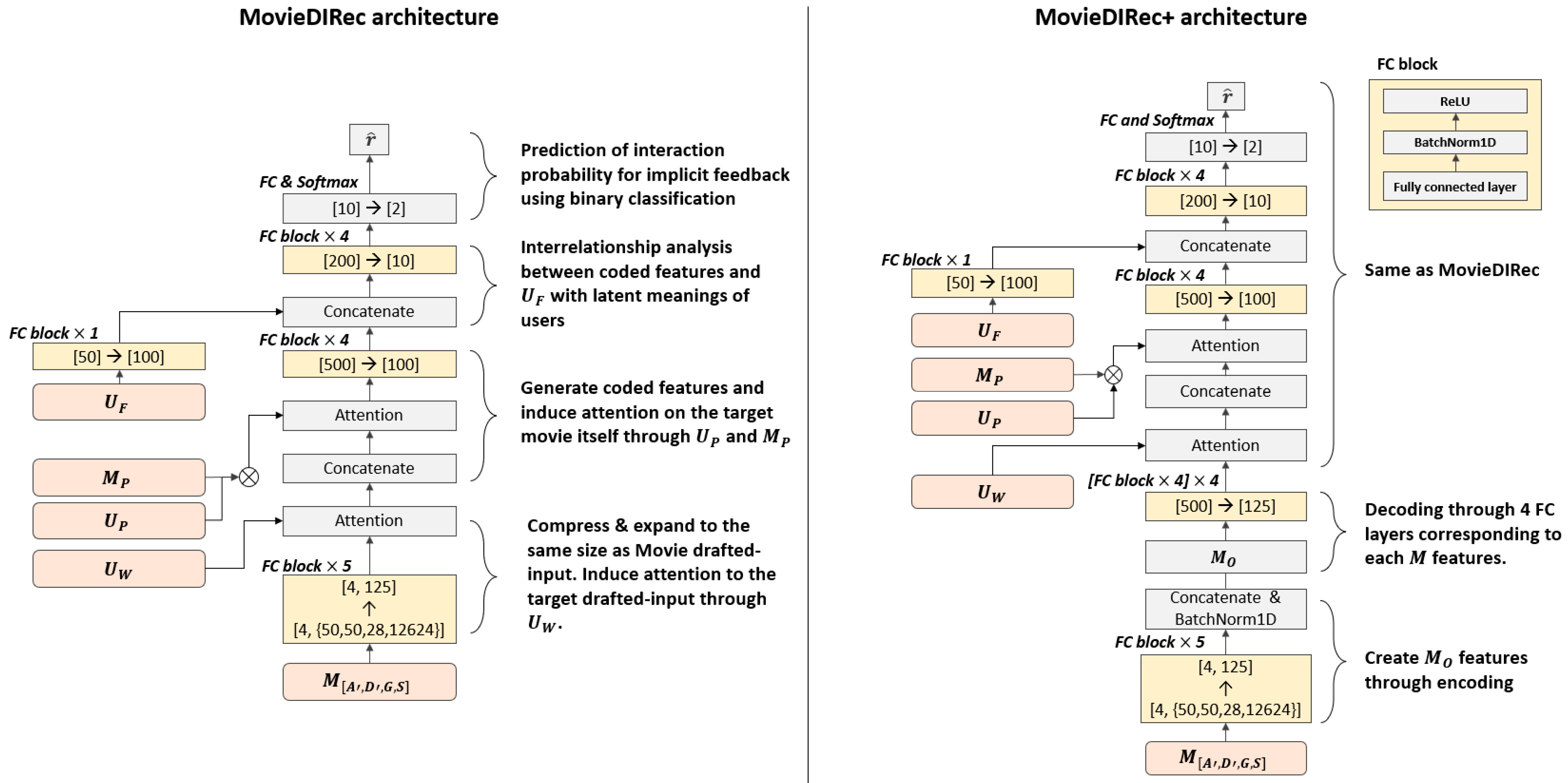
3.2. Proposed Methods: MovieDIRec and MovieDIRec+
4. Experiments
4.1. Metric
4.2. Setup
- VASP [4]: The author proposed a model ensembled by element-wise multiplication of NEASE and FLVAE as a VAE-based Top-N recommendation system.
- RaCT [5]: An efficient and scalable learning-to-rank algorithm was proposed by borrowing the actor–critic idea of reinforcement learning to approximate the ranking metric.
- RecVAE [6]: The authors followed the Mult-VAE model using multinomial distribution instead of Gaussian and Bernoulli distribution, which is generally used as the likelihood function in VAE, but improved the performance by modifying the Evidence Lower Bound (ELBO) formula and detailed architecture.
- CML [22]: By combining metric learning algorithms with collaborative filtering, the authors proposed a method to learn using similarity between user–user and user–item, and achieve significant speedup and approximate nearest-neighbor search with a slight decrease in accuracy.
4.3. Dataset
- D@1: All rating data;
- D@2, 3: Data(D@2) randomly extracted from 10 ratings per user to make Drafted-Input in D@1 and remaining data(D@3);
- D@4, 5: Data(D@4) extracted from D@3 of 10,000 Held-out users and the rest of the data (D@5);
- D@6, 7: Data(D@6) extracted at a rate of 10% from D@5 for training and data(D@7) extracted from 20% of the remaining data for testing for input training;
- D@8: Data extracted at a rate of 12% from D@4 for validation/test.
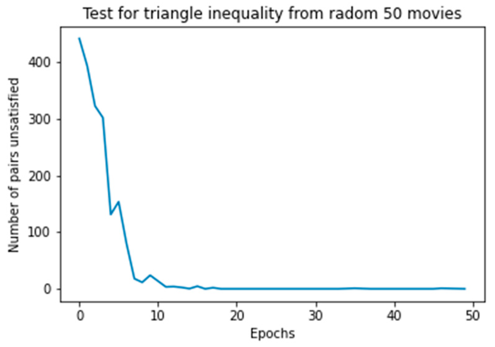
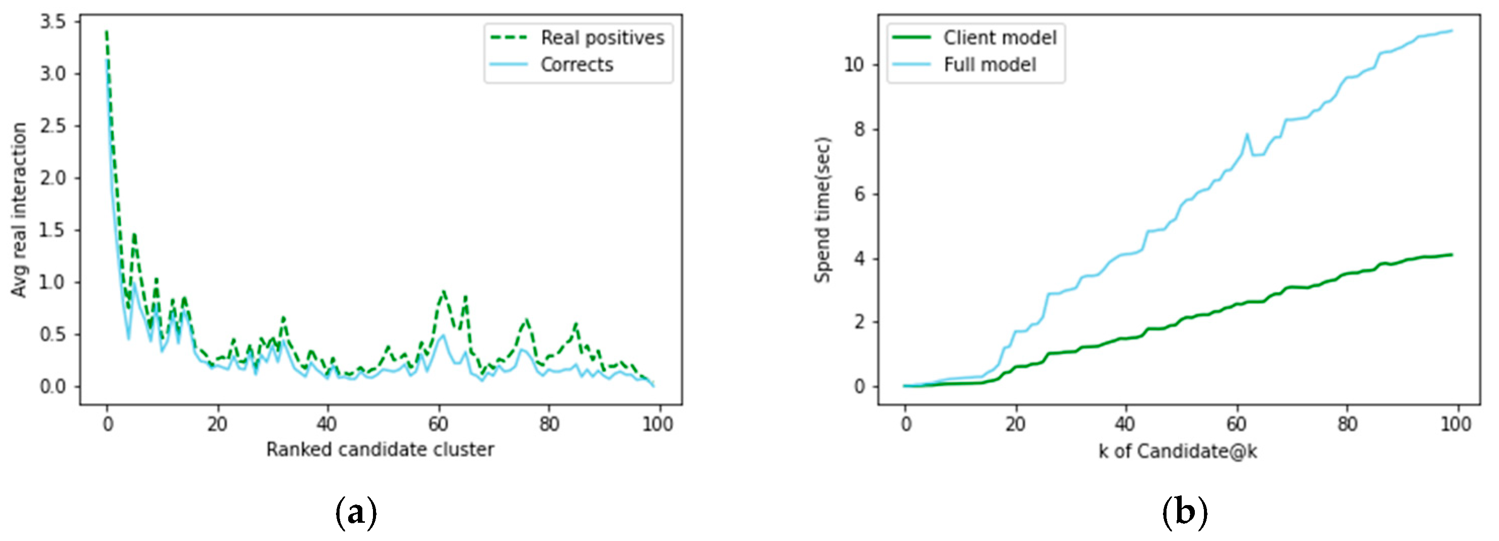
4.4. Results and Analysis
5. Conclusions
Author Contributions
Funding
Institutional Review Board Statement
Informed Consent Statement
Data Availability Statement
Conflicts of Interest
References
- An, H.-W.; Moon, N. Design of recommendation system for tourist spot using sentiment analysis based on CNN-LSTM. J. Ambient. Intell. Humaniz. Comput. 2019, 1–11. [Google Scholar] [CrossRef]
- Wei, T.; Wu, Z.; Li, R.; Hu, Z.; Feng, F.; He, X.; Sun, Y.; Wang, W. Fast Adaptation for Cold-start Collaborative Filtering with Meta-learning. In Proceedings of the 2020 IEEE International Conference on Data Mining (ICDM), Sorrento, Italy, 17–20 November 2020; IEEE: Piscataway, NJ, USA, 2020. [Google Scholar]
- Ammad-Ud-Din, M.; Ivannikova, E.; Khan, S.A.; Oyomno, W.; Fu, Q.; Tan, K.E.; Flanagan, A. Federated collaborative filtering for privacy-preserving personalized recommendation system. arXiv 2019, arXiv:1901.09888. Available online: https://arxiv.org/abs/1901.09888 (accessed on 1 September 2021).
- Vančura, V.; Kordík, P. Deep variational autoencoder with shallow parallel path for top-N recommendation (VASP). arXiv 2021, arXiv:2102.05774. Available online: https://arxiv.org/abs/2102.05774 (accessed on 2 September 2021).
- Lobel, S.; Li, C.; Gao, J.; Carin, L. Towards Amortized Ranking-Critical Training for Collaborative Filtering. arXiv 2019, arXiv:1906.04281. Available online: https://arxiv.org/abs/1906.04281 (accessed on 2 September 2021).
- Shenbin, I.; Alekseev, A.; Tutubalina, E.; Malykh, V.; Nikolenko, S.I. RecVAE: A new variational autoencoder for top-n recommendations with implicit feedback. In Proceedings of the 13th International Conference on Web Search and Data Mining, Houston, TX, USA, 3–7 February 2020. [Google Scholar]
- Steck, H. Embarrassingly shallow autoencoders for sparse data. In Proceedings of the World Wide Web Conference, San Francisco, CA, USA, 13–17 May 2019. [Google Scholar]
- Liang, D.; Krishnan, R.G.; Hoffman, M.D.; Jebara, T. Variational autoencoders for collaborative filtering. In Proceedings of the 2018 World Wide Web Conference, Lyon, France, 23–27 April 2018. [Google Scholar]
- Kim, J.; Park, J.; Shin, M.; Lee, J.; Moon, N. The Method for Generating Recommended Candidates through Prediction of Multi-Criteria Ratings Using CNN-BiLSTM. J. Inf. Process. Syst. 2021, 17, 707–720. [Google Scholar]
- Paul, C.; Adams, J.; Sargin, E. Deep neural networks for youtube recommendations. In Proceedings of the 10th ACM Conference on Recommender Systems, Boston, MA, USA, 15–19 September 2016. [Google Scholar]
- Vartak, M.; Thiagarajan, A.; Miranda, C.; Bratman, J.; Larochelle, H. A Meta-Learning Perspective on Cold-Start Recommendations for Items. 2017. Available online: https://papers.nips.cc/paper/7266-a-meta-learning-perspective-on-cold-start-recommendations-for-items.pdf (accessed on 5 September 2021).
- Bobadilla, J.; Alonso, S.; Hernando, A. Deep Learning Architecture for Collaborative Filtering Recommender Systems. Appl. Sci. 2020, 10, 2441. [Google Scholar] [CrossRef] [Green Version]
- Harper, F.M.; Konstan, J.A. The movielens datasets: History and context. ACM Trans. Interact. Intell. Syst. 2015, 5, 1–19. [Google Scholar] [CrossRef]
- Vozalis, M.G.; Margaritis, K.G. Using SVD and demographic data for the enhancement of generalized Collaborative Filtering. Inf. Sci. 2007, 177, 3017–3037. [Google Scholar] [CrossRef]
- Huseyin, P.; Du, W. SVD-based collaborative filtering with privacy. In Proceedings of the 2005 ACM Symposium on Applied Computing, Santa Fe, NM, USA, 13–17 March 2005. [Google Scholar]
- Barathy, R.; Chitra, P. Applying matrix factorization in collaborative filtering recommender systems. In Proceedings of the 2020 6th International Conference on Advanced Computing and Communication Systems (ICACCS), Coimbatore, India, 6–7 March 2020; IEEE: Piscataway, NJ, USA, 2020. [Google Scholar]
- Lourenco, J.; Varde, A.S. Item-Based Collaborative Filtering and Association Rules for a Baseline Recommender in E-Commerce. In Proceedings of the 2020 IEEE International Conference on Big Data (Big Data), Atlanta, GA, USA, 10–13 December 2020; IEEE: Piscataway, NJ, USA, 2020. [Google Scholar]
- Yan, C.; Zhang, Y.; Zhong, W.; Zhang, C.; Xin, B. A truncated SVD-based ARIMA model for multiple QoS prediction in mobile edge computing. Tsinghua Sci. Technol. 2021, 27, 315–324. [Google Scholar] [CrossRef]
- Zhuang, F.; Zhang, Z.; Qian, M.; Shi, C.; Xie, X.; He, Q. Representation learning via Dual-Autoencoder for recommendation. Neural Netw. 2017, 90, 83–89. [Google Scholar] [CrossRef] [PubMed]
- Yuan, F.; Yao, L.; Benatallah, B. Adversarial collaborative auto-encoder for top-n recommendation. In Proceedings of the 2019 International Joint Conference on Neural Networks (IJCNN), Budapest, Hungary, 14–19 July 2019; IEEE: Piscataway, NJ, USA, 2019. [Google Scholar]
- Devlin, J.; Chang, M.W.; Lee, K.; Toutanova, K. Bert: Pre-training of deep bidirectional transformers for language understanding. arXiv 2018, arXiv:1810.04805. Available online: https://arxiv.org/abs/1810.04805 (accessed on 10 September 2021).
- Hsieh, C.K.; Yang, L.; Cui, Y.; Lin, T.Y.; Belongie, S.; Estrin, D. Collaborative metric learning. In Proceedings of the 26th International Conference on World Wide Web, Perth, Australia, 3–7 April 2017. [Google Scholar]
- Kulis, B. Metric Learning: A Survey. Found. Trends Mach. Learn. 2013, 5, 287–364. [Google Scholar] [CrossRef]
- Xing, E.; Jordan, M.; Russell, S.J.; Ng, A. Distance metric learning with application to clustering with side-information. Adv. Neural Inf. Process. Syst. 2002, 15, 521–528. [Google Scholar]
- Daeryong, K.; Suh, B. Enhancing VAEs for collaborative filtering: Flexible priors & gating mechanisms. In Proceedings of the 13th ACM Conference on Recommender Systems, Copenhagen, Denmark, 16–20 September 2019. [Google Scholar]


| %Density Train | #Interaction Test | #User | #Movie | #Rating | %Train/Test | |
|---|---|---|---|---|---|---|
| VASP [4] | 0.29% | 14.63 | 136,677 | 20,108 | 10M | 80%/20% |
| RaCT [5] | - | - | 136,677 | 20,108 | 10M | - |
| RecVAE [6] | 0.28% | 14.61 | 136,677 | 20,720 | 9,990,682 | 80%/20% |
| CML [22] | 0.29% | 15.31 | 129,797 | 20,709 | 9,939,873 | 80%/20% |
| Ours | 0.26% | 14.87 | 51,869 | 4714 | 6,429,862 | 10%/12% |
| %Density Train | |||||
|---|---|---|---|---|---|
| VASP [4] | 0.29% | - | 0.448 | 0.414 | 0.552 |
| RaCT [5] | - | - | 0.403 | 0.403 | 0.543 |
| RecVAE [6] | 0.28% | - | 0.442 | 0.414 | 0.553 |
| CML [22] | 0.29% | 0.5301 | - | - | 0.4665 |
| MovieDIRec | 0.26% | 0.6113 | 0.4567 | 0.5223 | 0.5319 |
| MovieDIRec+ | 0.6246 | 0.4790 | 0.5532 | 0.5634 | |
| MovieDIRec * | 0.6136 | 0.4789 | 0.5189 | 0.5342 | |
| MovieDIRec+ * | 0.6535 | 0.5132 | 0.5049 | 0.5276 |
| %Density Train | |||||
|---|---|---|---|---|---|
| MovieDIRec | 3.85% | 0.7305 | 0.5908 | 0.5669 | 0.6384 |
| MovieDIRec+ | 0.7305 | 0.5910 | 0.5710 | 0.6443 | |
| MovieDIRec * | 0.7522 | 0.6368 | 0.5516 | 0.5851 | |
| MovieDIRec+ * | 0.7528 | 0.6293 | 0.5540 | 0.5972 |
| Total + Full Model | Total + Client Model | Candidate@10 + Full Model | Candidate@10 + Client Model | |
|---|---|---|---|---|
| Spend time | 5.1121 s | 2.9961 s | 0.2566 s | 0.1278 s |
| vs. Full model | - | ↓41.39% | ↓94.98% | ↓97.50% |
| Input size (91,514 movies) | 1.9 GB | 183 MB | 190 MB | 19 MB |
Publisher’s Note: MDPI stays neutral with regard to jurisdictional claims in published maps and institutional affiliations. |
© 2021 by the authors. Licensee MDPI, Basel, Switzerland. This article is an open access article distributed under the terms and conditions of the Creative Commons Attribution (CC BY) license (https://creativecommons.org/licenses/by/4.0/).
Share and Cite
An, H.; Kim, D.; Lee, K.; Moon, N. MovieDIRec: Drafted-Input-Based Recommendation System for Movies. Appl. Sci. 2021, 11, 10412. https://doi.org/10.3390/app112110412
An H, Kim D, Lee K, Moon N. MovieDIRec: Drafted-Input-Based Recommendation System for Movies. Applied Sciences. 2021; 11(21):10412. https://doi.org/10.3390/app112110412
Chicago/Turabian StyleAn, Hyeonwoo, Daeyeol Kim, Kwangkee Lee, and Nammee Moon. 2021. "MovieDIRec: Drafted-Input-Based Recommendation System for Movies" Applied Sciences 11, no. 21: 10412. https://doi.org/10.3390/app112110412