
Assembly Quality Detection Based on Class-Imbalanced Semi-Supervised Learning

Abstract
:1. Introduction
2. Class-Imbalanced Semi-Supervised Learning
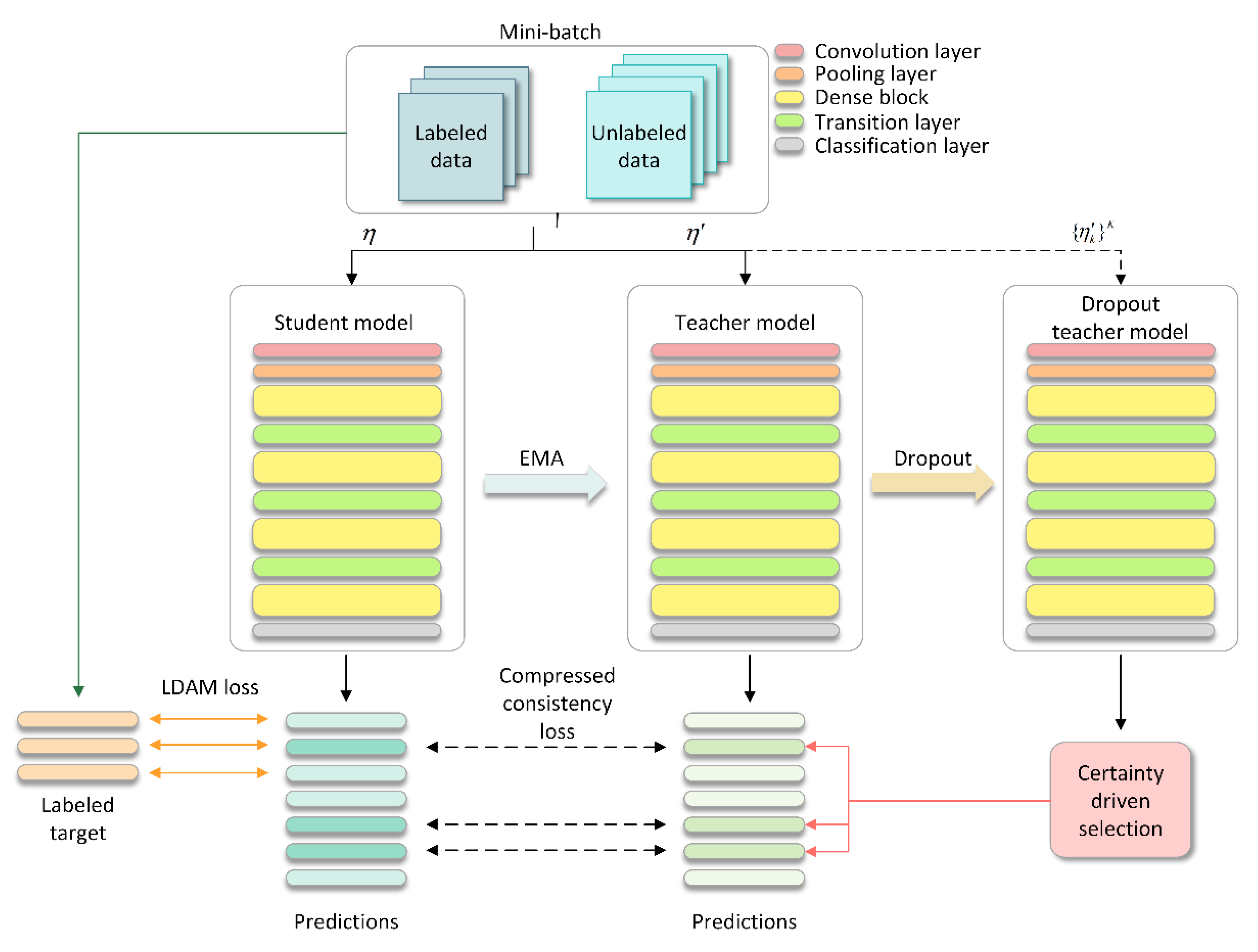
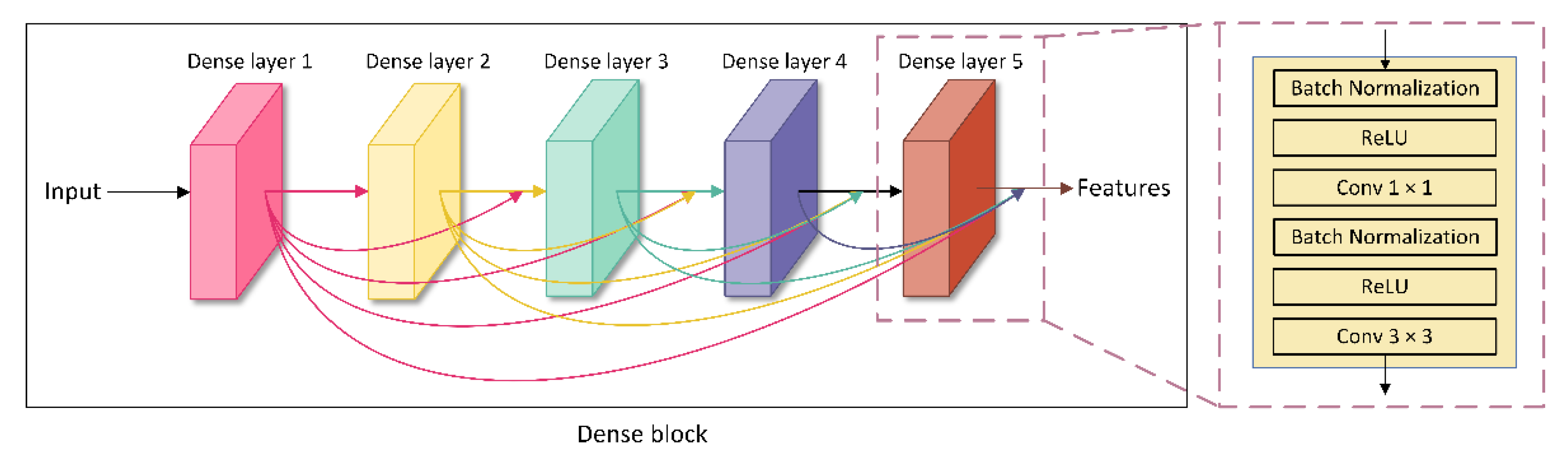
2.1. Model Framework for Assembly Quality Detection
| Algorithm 1 Training of the proposed method | |
| Input:Dl, Du, B, bl, β, K | |
| Initialization:θs, θt | |
| for | iter = 1 T do |
 | Sample batches |
| Student prediction | |
| Dropout samplings | |
| Teacher prediction | |
| Compute uncertainty | |
| Rearrange in ascending order | |
| Update the student model | |
| Update the teacher model | |
| end | |
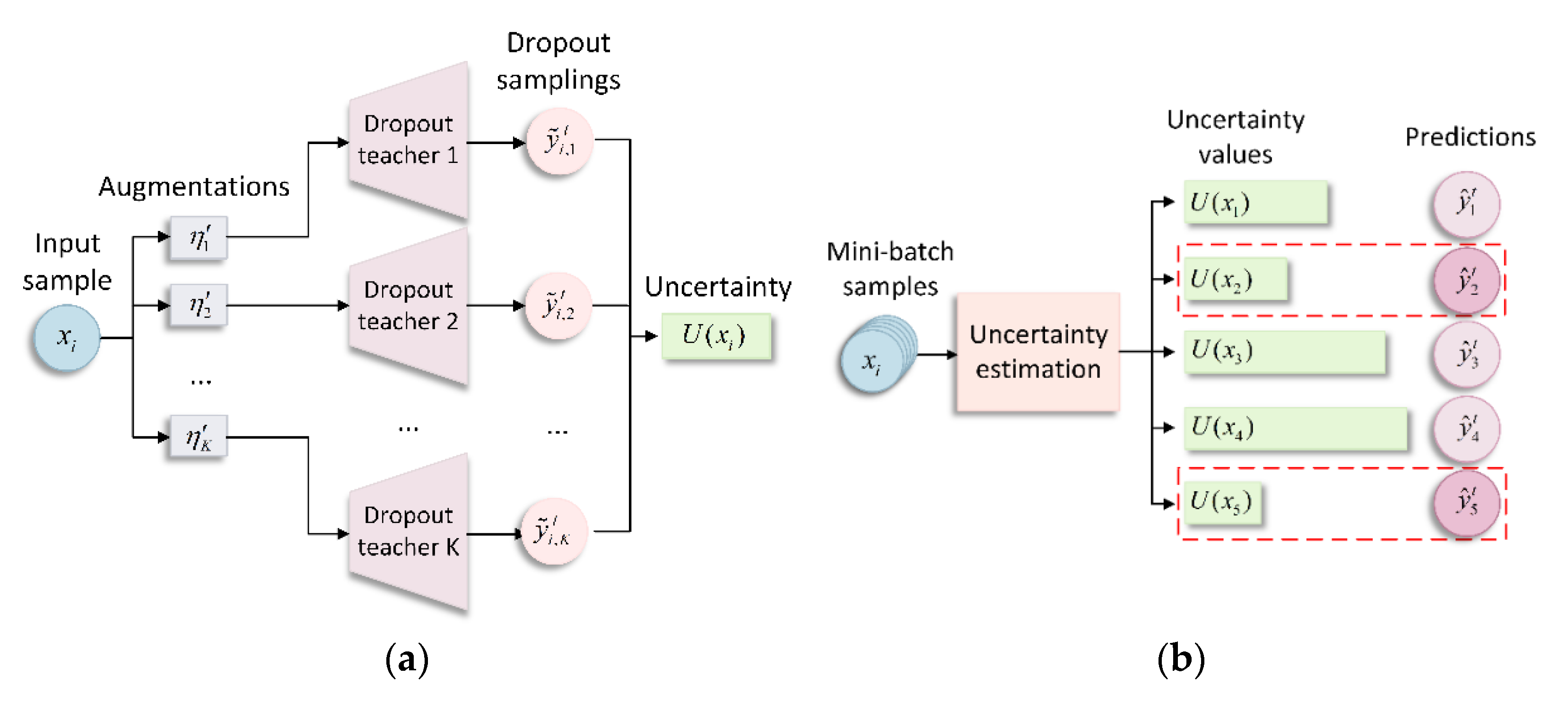
2.2. Certainty Driven Selection
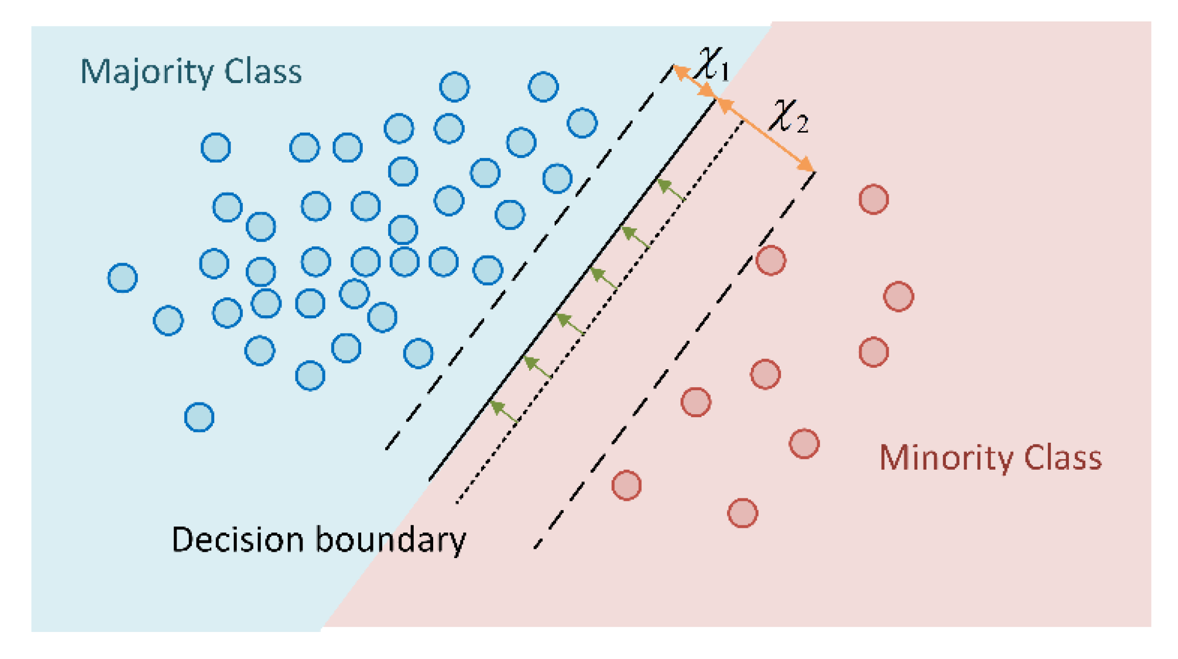
2.3. Class-Imbalanced Learning
3. Results
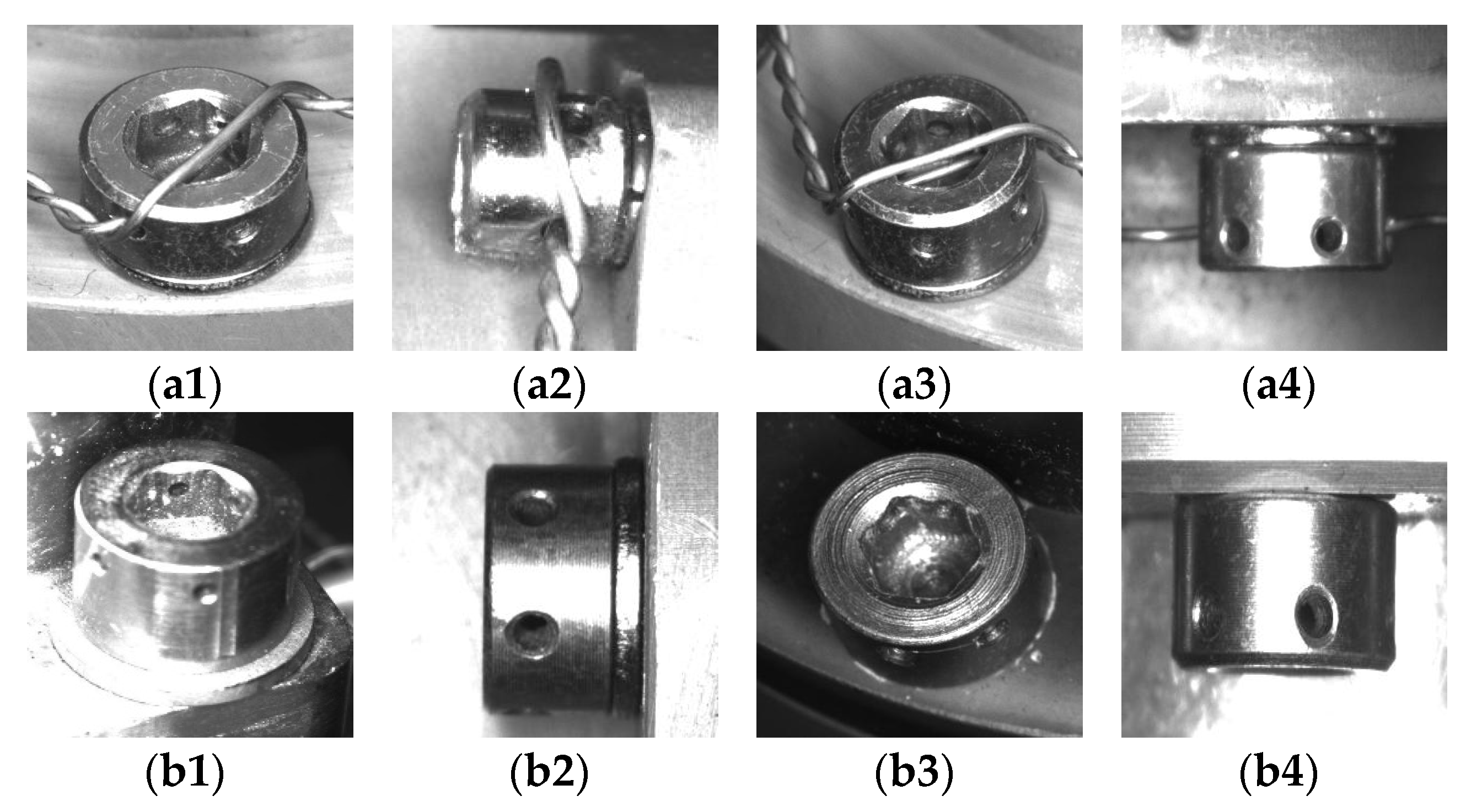
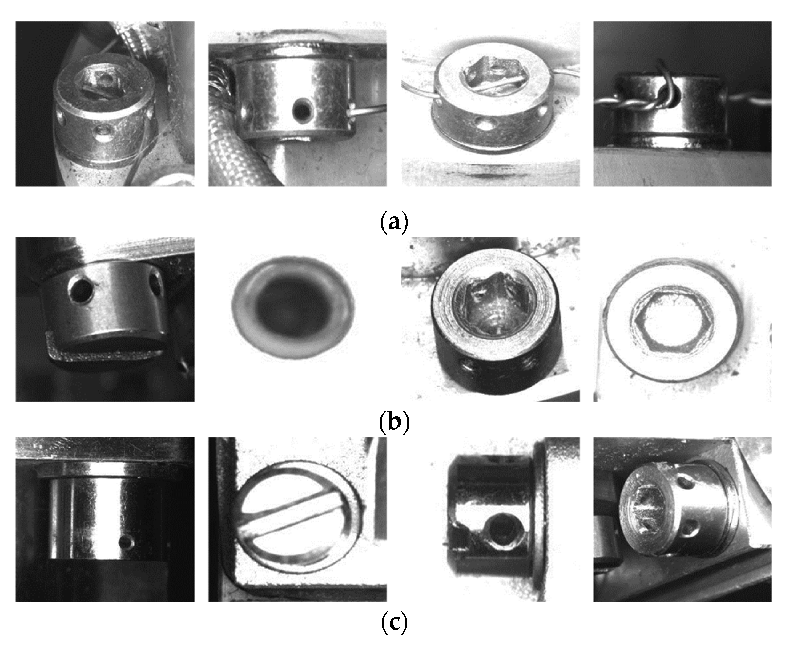
3.1. Dataset
3.2. Training Settings and Metrics
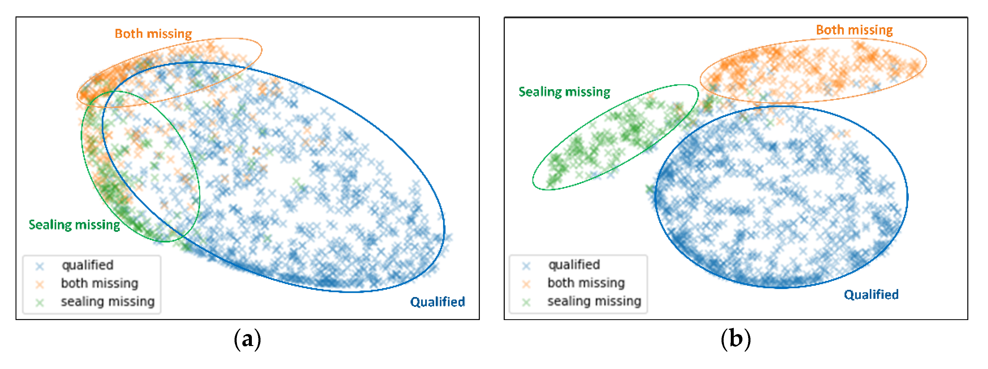
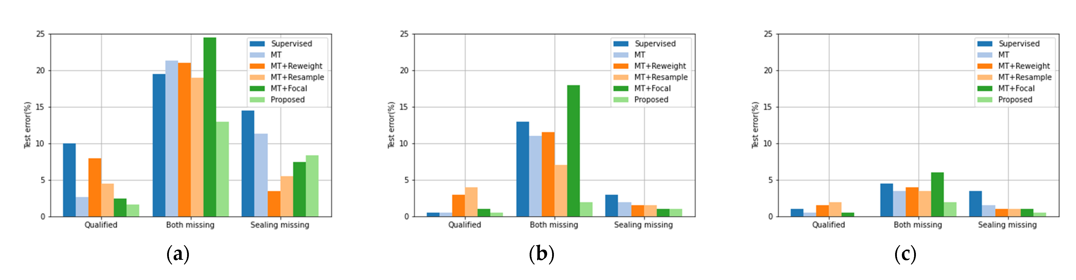
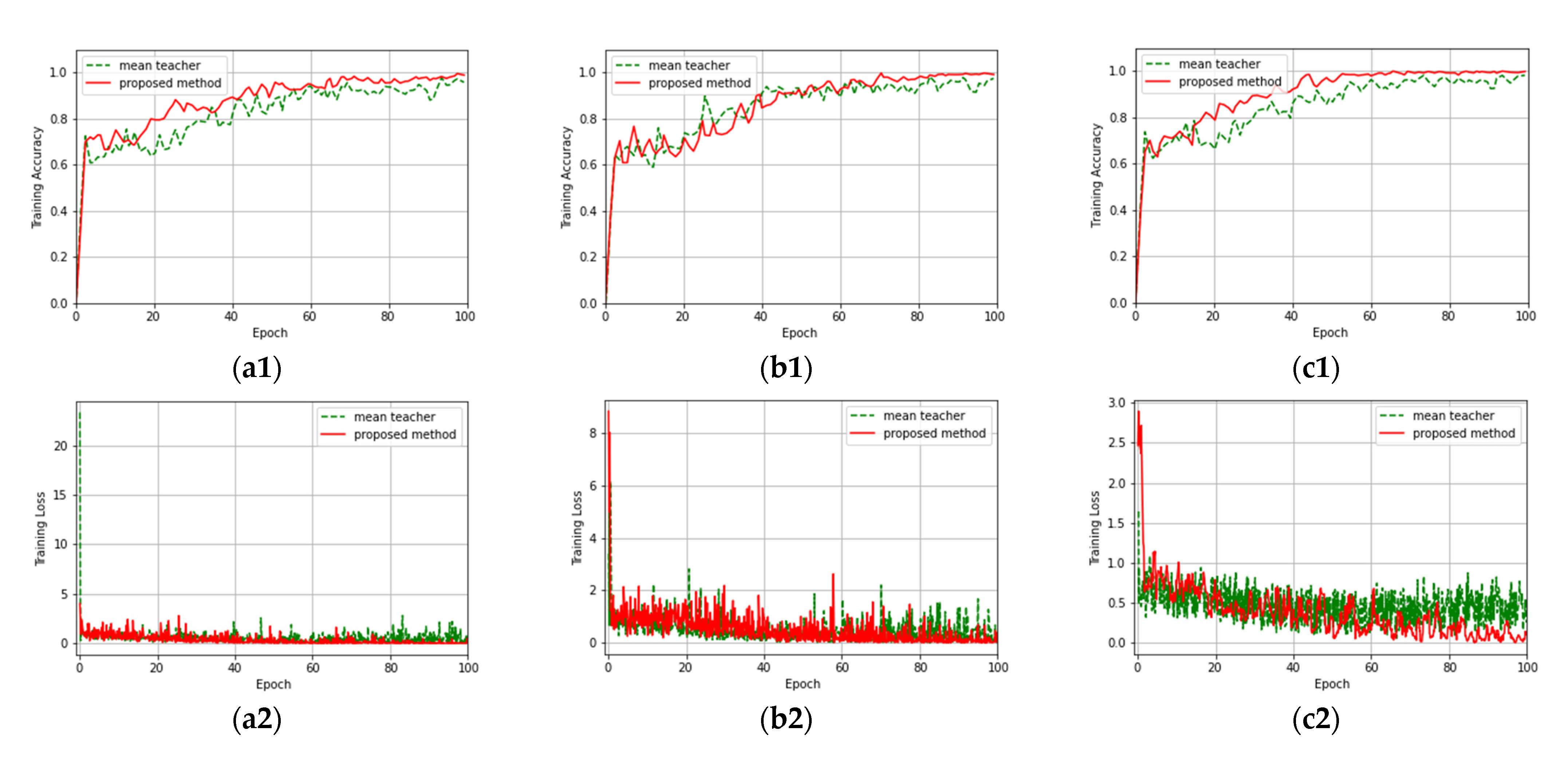
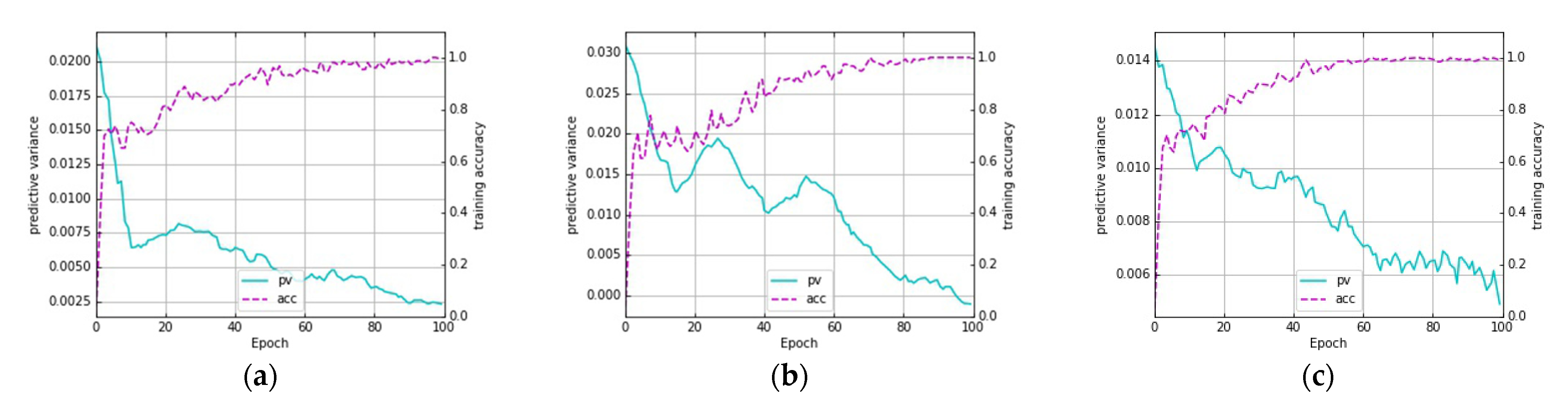
3.3. Experimental Results
4. Conclusions
Author Contributions
Funding
Institutional Review Board Statement
Informed Consent Statement
Data Availability Statement
Acknowledgments
Conflicts of Interest
References
- Feng, H.; Jiang, Z.; Xie, F.; Yang, P.; Shi, J.; Chen, L. Automatic Fastener Classification and Defect Detection in Vision-Based Railway Inspection Systems. IEEE Trans. Instrum. Meas. 2014, 63, 877–888. [Google Scholar] [CrossRef]
- Liu, L.; Zhou, F.; He, Y. Automated Visual Inspection System for Bogie Block Key Under Complex Freight Train Environment. IEEE Trans. Instrum. Meas. 2016, 65, 2–14. [Google Scholar] [CrossRef]
- Wojciechowski, J.; Suszynski, M. Optical Scanner Assisted Robotic Assembly. Assem. Autom. 2017, 37, 434–441. [Google Scholar] [CrossRef]
- Suszynski, M.; Wojciechowski, J.; Zurek, J. No Clamp Robotic Assembly with Use of Point Cloud Data from Low-Cost Triangulation Scanner. Teh. Vjesn. Tech. Gaz. 2018, 25, 904–909. [Google Scholar] [CrossRef]
- Reyno, T.; Marsden, C.; Wowk, D. Surface Damage Evaluation of Honeycomb Sandwich Aircraft Panels Using 3D Scanning Technology. NDT E Int. 2018, 97, 11–19. [Google Scholar] [CrossRef]
- Park, J.; Huynh, T.; Choi, S.; Kim, J. Vision-Based Technique for Bolt-Loosening Detection in Wind Turbine Tower. Wind. Struct. Int. J. 2015, 21, 709–726. [Google Scholar] [CrossRef]
- Gibert, X.; Patel, V.M.; Chellappa, R. Deep Multitask Learning for Railway Track Inspection. IEEE Trans. Intell. Transp. Syst. 2017, 18, 153–164. [Google Scholar] [CrossRef] [Green Version]
- Chen, J.; Liu, Z.; Wang, H.; Nunez, A.; Han, Z. Automatic Defect Detection of Fasteners on the Catenary Support Device Using Deep Convolutional Neural Network. IEEE Trans. Instrum. Meas. 2018, 67, 257–269. [Google Scholar] [CrossRef] [Green Version]
- Kang, G.; Gao, S.; Yu, L.; Zhang, D. Deep Architecture for High-Speed Railway Insulator Surface Defect Detection: Denoising Autoencoder With Multitask Learning. IEEE Trans. Instrum. Meas. 2019, 68, 2679–2690. [Google Scholar] [CrossRef]
- Chang, L.; Liu, Z.; Shen, Y.; Zhang, G. Novel Multistate Fault Diagnosis and Location Method for Key Components of High-Speed Trains. IEEE Trans. Ind. Electron. 2021, 68, 3537–3547. [Google Scholar] [CrossRef]
- Wang, C.; Xu, Z. An Intelligent Fault Diagnosis Model Based on Deep Neural Network for Few-Shot Fault Diagnosis. Neurocomputing 2021, 456, 550–562. [Google Scholar] [CrossRef]
- Zhang, S.; Ye, F.; Wang, B.; Habetler, T.G. Semi-Supervised Bearing Fault Diagnosis and Classification Using Variational Autoencoder-Based Deep Generative Models. IEEE Sens. J. 2021, 21, 6476–6486. [Google Scholar] [CrossRef]
- Tang, L.; Xuan, J.; Shi, T.; Zhang, Q. EnvelopeNet: A Robust Convolutional Neural Network with Optimal Kernels for Intelligent Fault Diagnosis of Rolling Bearings. Measurement 2021, 180, 109563. [Google Scholar] [CrossRef]
- Liu, C.; Wu, Y.; Liu, J.; Sun, Z.; Xu, H. Insulator Faults Detection in Aerial Images from High-Voltage Transmission Lines Based on Deep Learning Model. Appl. Sci. 2021, 11, 4647. [Google Scholar] [CrossRef]
- Gao, Z.; Yang, G.; Li, E.; Liang, Z. Novel Feature Fusion Module-Based Detector for Small Insulator Defect Detection. IEEE Sens. J. 2021, 21, 16807–16814. [Google Scholar] [CrossRef]
- Liu, J.; Liu, C.; Wu, Y.; Xu, H.; Sun, Z. An Improved Method Based on Deep Learning for Insulator Fault Detection in Diverse Aerial Images. Energies 2021, 14, 4365. [Google Scholar] [CrossRef]
- Wang, Y.; Yao, Q.; Kwok, J.T.; Ni, L.M. Generalizing from a Few Examples: A Survey on Few-Shot Learning. ACM Comput. Surv. 2020, 53, 63:1–63:34. [Google Scholar] [CrossRef]
- Wu, J.; Zhao, Z.; Sun, C.; Yan, R.; Chen, X. Few-Shot Transfer Learning for Intelligent Fault Diagnosis of Machine. Measurement 2020, 166, 108202. [Google Scholar] [CrossRef]
- Gao, F.; Ma, F.; Wang, J.; Sun, J.; Yang, E.; Zhou, H. Semi-Supervised Generative Adversarial Nets with Multiple Generators for SAR Image Recognition. Sensors 2018, 18, 2706. [Google Scholar] [CrossRef] [Green Version]
- Cabrera, D.; Sancho, F.; Long, J.; Sánchez, R.; Zhang, S.; Cerrada, M.; Li, C. Generative Adversarial Networks Selection Approach for Extremely Imbalanced Fault Diagnosis of Reciprocating Machinery. IEEE Access 2019, 7, 70643–70653. [Google Scholar] [CrossRef]
- Li, X.; Zhang, W.; Ding, Q. Cross-Domain Fault Diagnosis of Rolling Element Bearings Using Deep Generative Neural Networks. IEEE Trans. Ind. Electron. 2019, 66, 5525–5534. [Google Scholar] [CrossRef]
- Zhou, F.; Song, Y.; Liu, L.; Zheng, D. Automated Visual Inspection of Target Parts for Train Safety Based on Deep Learning. IET Intell. Transp. Syst. 2018, 12, 550–555. [Google Scholar] [CrossRef]
- Chapelle, O.; Schölkopf, B.; Zien, A. Semi-Supervised Learning; MIT Press: Cambridge, MA, USA, 2009. [Google Scholar]
- Sajjadi, M.; Javanmardi, M.; Tasdizen, T. Regularization With Stochastic Transformations and Perturbations for Deep Semi-Supervised Learning. In Proceedings of the 30th International Conference on Neural Information Processing Systems, Barcelona, Spain, 5–10 December 2016; Curran Associates Inc.: Red Hook, NY, USA, 2016. [Google Scholar]
- Laine, S.; Aila, T. Temporal Ensembling for Semi-Supervised Learning. In Proceedings of the 5th International Conference on Learning Representations, ICLR 2017, Toulon, France, 24–26 December 2017. [Google Scholar]
- Tarvainen, A.; Valpola, H. Mean Teachers Are Better Role Models: Weight-Averaged Consistency Targets Improve Semi-Supervised Deep Learning Results. In Proceedings of the 31st International Conference on Neural Information Processing Systems, Long Beach, CA, USA, 4–9 December 2017; Curran Associates Inc.: Red Hook, NY, USA, 2017. [Google Scholar]
- Kim, J.; Hur, Y.; Park, S.; Yang, E.; Hwang, S.; Shin, J. Distribution Aligning Refinery of Pseudo-Label for Imbalanced Semi-Supervised Learning. In Proceedings of the 34th International Conference on Neural Information Processing Systems, Online, 6–12 December 2020; Curran Associates Inc.: Red Hook, NY, USA, 2020. [Google Scholar]
- Cao, K.; Wei, C.; Gaidon, A.; Arechiga, N.; Ma, T. Learning Imbalanced Datasets with Label-Distribution-Aware Margin Loss. In Proceedings of the 33rd International Conference on Neural Information Processing Systems, Vancouver, BC, Canada, 8–14 December 2019; Curran Associates Inc.: Red Hook, NY, USA, 2019. [Google Scholar]
- Huang, G.; Liu, Z.; Maaten, L.V.D.; Weinberger, K.Q. Densely Connected Convolutional Networks. In Proceedings of the 2017 IEEE Conference on Computer Vision and Pattern Recognition (CVPR), Honolulu, HI, USA, 21–26 July 2017; pp. 2261–2269. [Google Scholar]
- Gal, Y.; Ghahramani, Z. Dropout as a Bayesian Approximation: Representing Model Uncertainty in Deep Learning. In Proceedings of the 33rd International Conference on Machine Learning, New York, NY, USA, 19–24 June 2016. [Google Scholar]
- Gal, Y.; Ghahramani, Z. Bayesian Convolutional Neural Networks with Bernoulli Approximate Variational Inference. In Proceedings of the 4th International Conference on Learning Representations, ICLR2016. Caribe Hilton, San Juan, Puerto Rico, 2–4 May 2016. [Google Scholar]
- Liu, L.; Li, Y.; Tan, R.T. Decoupled Certainty-Driven Consistency Loss for Semi-Supervised Learning. arXiv 2020, arXiv:1901.05657. [Google Scholar]
- He, H.; Garcia, E.A. Learning from Imbalanced Data. Knowl. Data Eng. IEEE Trans. 2008, 21, 1263–1284. [Google Scholar] [CrossRef]
- Buda, M.; Maki, A.; Mazurowski, M.A. A Systematic Study of the Class Imbalance Problem in Convolutional Neural Networks. Neural Netw. 2018, 106, 249–259. [Google Scholar] [CrossRef] [Green Version]
- Cui, Y.; Jia, M.; Lin, T.-Y.; Song, Y.; Belongie, S. Class-Balanced Loss Based on Effective Number of Samples. In Proceedings of the 2019 IEEE Conference on Computer Vision and Pattern Recognition (CVPR), Long Beach, CA, USA, 16–20 June 2019. [Google Scholar]
- Deng, J.; Dong, W.; Socher, R.; Li, L.; Li, K.; Li, F.-F. ImageNet: A Large-Scale Hierarchical Image Database. In Proceedings of the 2009 IEEE Conference on Computer Vision and Pattern Recognition, Miami, FL, USA, 20 June 2009; pp. 248–255. [Google Scholar]
- Huang, C.; Li, Y.; Loy, C.C.; Tang, X. Learning Deep Representation for Imbalanced Classification. In Proceedings of the 2016 IEEE Conference on Computer Vision and Pattern Recognition (CVPR), Las Vegas, NV, USA, 26 June–1 July 2016; pp. 5375–5384. [Google Scholar]
- Branco, P.; Torgo, L.; Ribeiro, R.P. A Survey of Predictive Modeling on Imbalanced Domains. ACM Comput. Surv. 2016, 49, 1–50. [Google Scholar] [CrossRef]
- Lin, T.-Y.; Goyal, P.; Girshick, R.; He, K.; Dollár, P. Focal Loss for Dense Object Detection. In Proceedings of the 2017 IEEE International Conference on Computer Vision, Venice, Italy, 22–19 October 2017; pp. 2980–2988. [Google Scholar]
- Van der Maaten, L.; Hinton, G. Visualizing Data Using T-SNE. J. Mach. Learn. Res. 2008, 9, 2579–2605. [Google Scholar]


| Class | Training Set | Testing Set | ||
|---|---|---|---|---|
| Qualified | 1136 | 2272 | 5680 | 100 |
| Both missing | 311 | 622 | 1555 | 100 |
| Sealing missing | 216 | 432 | 1080 | 100 |
| Unlabeled | 15,000 | 13,337 | 8348 | - |
| Methods | ||||||
| bACC | GM | bACC | GM | bACC | GM | |
| Supervised | 85.34 ± 0.94 | 85.10 ± 0.99 | 94.50 ± 0.42 | 94.32 ± 0.45 | 97.00 ± 0.09 | 96.98 ± 0.09 |
| MT | 88.22 ± 0.45 | 87.87 ± 0.47 | 95.50 ± 0.52 | 95.37 ± 0.54 | 98.16 ± 0.05 | 98.16 ± 0.05 |
| MT + Reweight | 89.34 ± 0.66 | 88.98 ± 0.70 | 94.67 ± 0.56 | 94.50 ± 0.61 | 97.84 ± 0.05 | 97.82 ± 0.04 |
| MT + Resample | 90.34 ± 0.47 | 90.06 ± 0.29 | 95.84 ± 0.52 | 95.80 ± 0.53 | 97.84 ± 0.05 | 97.82 ± 0.05 |
| MT + Focal | 88.50 ± 0.81 | 87.86 ± 0.90 | 93.33 ± 0.28 | 92.95 ± 0.32 | 97.50 ± 0.09 | 97.46 ± 0.11 |
| Proposed method | 93.67 ± 0.27 | 93.57 ± 0.28 | 98.83 ± 0.14 | 98.83 ± 0.14 | 99.17 ± 0.07 | 98.99 ± 0.04 |
Publisher’s Note: MDPI stays neutral with regard to jurisdictional claims in published maps and institutional affiliations. |
© 2021 by the authors. Licensee MDPI, Basel, Switzerland. This article is an open access article distributed under the terms and conditions of the Creative Commons Attribution (CC BY) license (https://creativecommons.org/licenses/by/4.0/).
Share and Cite
Lu, Z.; Jiang, J.; Cao, P.; Yang, Y. Assembly Quality Detection Based on Class-Imbalanced Semi-Supervised Learning. Appl. Sci. 2021, 11, 10373. https://doi.org/10.3390/app112110373
Lu Z, Jiang J, Cao P, Yang Y. Assembly Quality Detection Based on Class-Imbalanced Semi-Supervised Learning. Applied Sciences. 2021; 11(21):10373. https://doi.org/10.3390/app112110373
Chicago/Turabian StyleLu, Zichen, Jiabin Jiang, Pin Cao, and Yongying Yang. 2021. "Assembly Quality Detection Based on Class-Imbalanced Semi-Supervised Learning" Applied Sciences 11, no. 21: 10373. https://doi.org/10.3390/app112110373