Wind Power Forecasting with Deep Learning Networks: Time-Series Forecasting ^†

Abstract

Studies have demonstrated that changes in the climate affect wind power forecasting under different weather conditions. Theoretically, accurate prediction of both wind power output and weather changes using statistics-based prediction models is difficult. In practice, traditional machine learning models can perform long-term wind power forecasting with a mean absolute percentage error (MAPE) of 10% to 17%, which does not meet the engineering requirements for our renewable energy project. Deep learning networks (DLNs) have been employed to obtain the correlations between meteorological features and power generation using a multilayer neural convolutional architecture with gradient descent algorithms to minimize estimation errors. This has wide applicability to the field of wind power forecasting. Therefore, this study aimed at the long-term (24–72-h ahead) prediction of wind power with an MAPE of less than 10% by using the Temporal Convolutional Network (TCN) algorithm of DLNs. In our experiment, we performed TCN model pretraining using historical weather data and the power generation outputs of a wind turbine from a Scada wind power plant in Turkey. The experimental results indicated an MAPE of 5.13% for 72-h wind power prediction, which is adequate within the constraints of our project. Finally, we compared the performance of four DLN-based prediction models for power forecasting, namely, the TCN, long short-term memory (LSTM), recurrent neural network (RNN), and gated recurrence unit (GRU) models. We validated that the TCN outperforms the other three models for wind power prediction in terms of data input volume, stability of error reduction, and forecast accuracy.

1. Introduction

With the increasingly serious global warming crisis and the burning of fossil fuels inducing air pollution and climate change, concerned parties have begun to invest in the development and application of renewable energy. European countries such as Denmark, Germany, and Sweden have invested in renewable energy through smart power grids, in which power suppliers and regional suppliers provide two-way complementary power supply and demand. The key technology of a smart power grid is power forecasting in relation to renewable energy, which is a clean power supply.

Many techniques have been applied to wind power forecasting to solve various problems, such as the fluctuations in power from wind farms for very short-term, short-term (from 30 min to day-ahead), medium-term (from day-ahead to month-ahead), and long-term (more than month-ahead) [1].

Wind power forecasting prediction models can be classified using the following three approaches: (1) the physical approach, in which weather changes are considered as deterministic events [1], (2) the statistical approach, in which weather changes are considered as a random process [2,3], and (3) the hybrid approach, which constitutes a weighted aggregation of the other two prediction models [4,5,6,7,8,9]. Compared with these three methods for wind power prediction problems, deep learning network (DLN) approaches, such as Boltzmann machines (RBM), long short-term memory (LSTM), temporal convolutional networks (TCN), and convolutional neural networks (CNN) have exhibited superior results and are generally considered as an alternative solution for wind power prediction [10,11]. These wind power forecasting schemes are summarised as

Table 1. Four Major Approaches for Wind Power Forecasting.

	Features	Limitations
Physical methods [1]	Physical methods for wind forecasting use numerical weather prediction (NWP) to predict weather, considering the effects of atmosphere, local terrain, and wind farm layout factors.	Needs a lot of weather experts to handle numerical weather data prediction. In case that accuracy of NWP is poor, the wind power generation forecasting becomes inaccurate.
Statistical methods [2,3]	Applies statistical methods to find the relationships between weather features and the predicted power. Statistical methods include Bayesian, regression, and auto regression integrated moving average (ARIMA) models.	A specific statistical method cannot handle complex weather conditions affected by atmosphere and environment factors. Thus, enhanced learning schemes such as random trees and GDBT are proposed in order to increase the accuracy for wind power prediction.
Hybrid methods [4,5,6,7,8,9]	Aggregate different weights of models to improve model performance by preserving advantages of each approach, such as combination of fuzzy logic approach, artificial neural network (ANN) and support vector machine (SVM), where SVM and fuzzy logic approach can complement each other and ensure superior results.	These hybrid models have problems with stable prediction as their complex learning architecture may cause low efficiency, long training times and even under-fitting.
Deep learning methods [10,11]	Use convolution operation to extract the features of time series data and predict the output using classification results. Multilayer neural networks for multiclass classification exhibited superior results in wind power forecasting applications. Compared with the traditional ANNs, deep learning neural networks do not need extra unsupervised networks or data preprocessing (e.g., decomposition).	The performance of the DLN model is constrained by the quality of data input and neural architecture design. To avoid constraints from data inputs, researchers have begun to study and propose new (NWP + DLN) models recently.

.

These developed models can perform long-term day-ahead wind power forecasting; however, forecasting schemes with a mean absolute percentage error (MAPE) between 12% and 17% [12,13] do not meet the engineering requirements. Thus, the development of an accurate and robust approach for wind power forecasting under varying climate conditions is still a challenge. Considering the increasing role of wind power in the renewable energy system, the research gaps and opportunities for wind power predicting are summarised as:

• Practically, most existing approaches to forecasting do not model the uncertainty of wind well. Thus, a high-accuracy wind power model needs high resolution weather data inputs generated by an NWP model, which is not a trivial task.
• Typically, deep learning-based neural networks for day ahead wind power forecasting outperform traditional neural networks such as ANN in renewable power forecasting problems, as these deep learning networks (DLNs) do not need extra data pre-processing, i.e., decomposition, in order to retrieve features from datasets.

Typically, wind power forecasting is subject to a power level output classification problem related to different spatial temporal weather data. Four major types of DLNs for time series data have been applied to wind power forecasting from the time-series sequence data input, namely the recurrent neural network (RNN), long short-term memory (LSTM), gated recurrence unit (GRU), and temporal convolutional network (TCN).

RNNs were the first neural networks to assist in analyzing and learning sequences of data. However, some problems with RNNs were raised during model training, including slow computation times on account of their recurrent nature. Particularly when using Relu or Tanh as the activation function, long sequence inputs (i.e., gradient exploding and vanishing problems) become difficult to process [14]. LSTM was later proposed to solve the gradient exploding and vanishing problems. Typically, LSTM is capable of learning lengthy time dependencies by using the forget, input, and output gates in the module. Similarly, LSTMs have some weaknesses, for example difficulty in applying the dropout algorithm. Dropout is a regularization method in which input and recurrent connections to the LSTM units are probabilistically excluded from activation and weight updates when training a network [15,16]. GRU is a type of RNN that, in certain cases, has advantages over LSTM. GRU uses less memory and is faster than LSTM, although LSTM is more accurate when using datasets with longer sequences [17,18,19].

In this study, we intend to answer the question of which deep machine learning methods for time series data input can predict day-ahead wind power generation with the smallest error. To investigate the forecast accuracy of day-ahead for wind turbines measured with a performance evaluation index (i.e., MAPE), we developed a feature-based learning model for wind power forecasting and trained TCNs [20,21,22,23] to learn meteorological features and identify the output class of power generation. We applied a multilayer neural convolutional architecture with gradient descent algorithms to minimize the estimation model error.

Four major types of sequence-to-sequence DLN models for wind power forecasting were compared to assess model performance. The experimental results demonstrated that the TCN outperforms canonical recurrent networks, LSTMs, RNNs, and GRUs across a diverse range of experiments and datasets. Thus, the TCN provides an effective means of accurately predicting power generation under varying climate conditions.

In summary, the primary contributions of this study are as follows:

▪

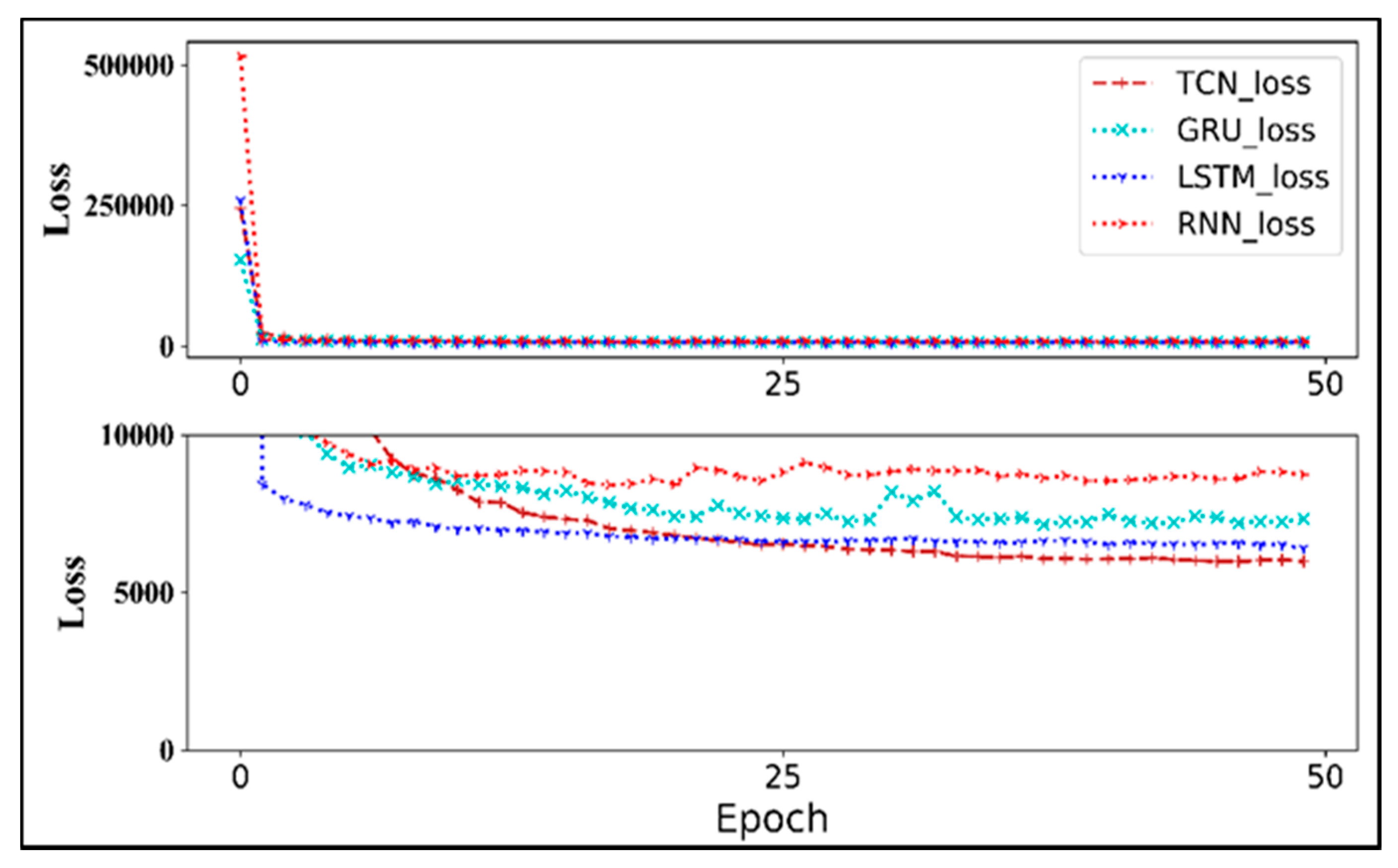
The optimal parameters of the models were investigated using evolutionary algorithms (EAs) in order to minimize convergence loss in the learning process.

▪

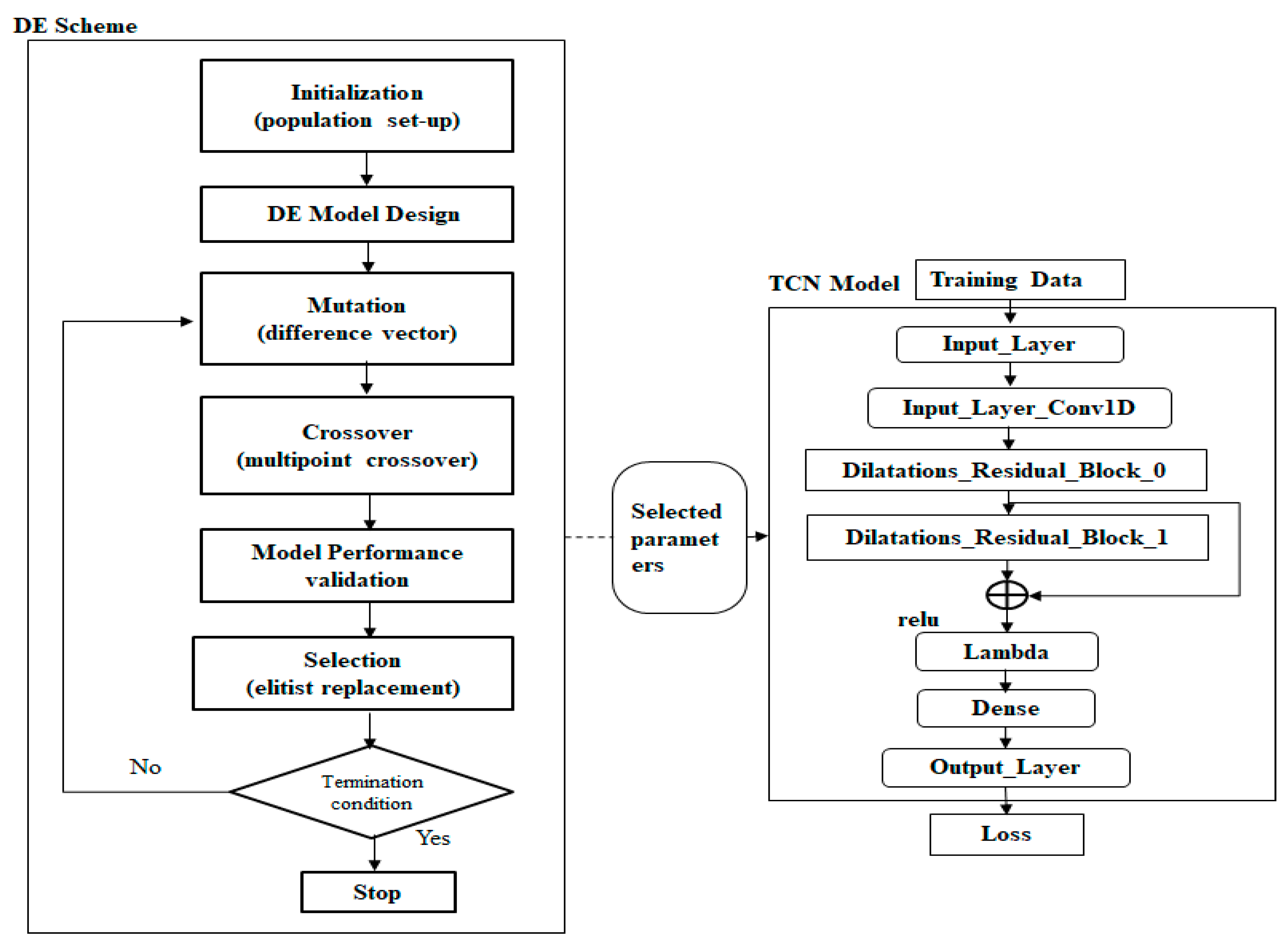
Four crucial architecture parameters for developed wind power prediction models were analysed, incorporating the differential evolution (DE) algorithm [16,17,18] in the learning process of the TCN model, namely, (i) number of filters, (ii) activation function, (iii) optimizer, and (iv) dilatation coefficient, in order to determine the initial model architecture for model training, according to the natural feature of TCN.

▪

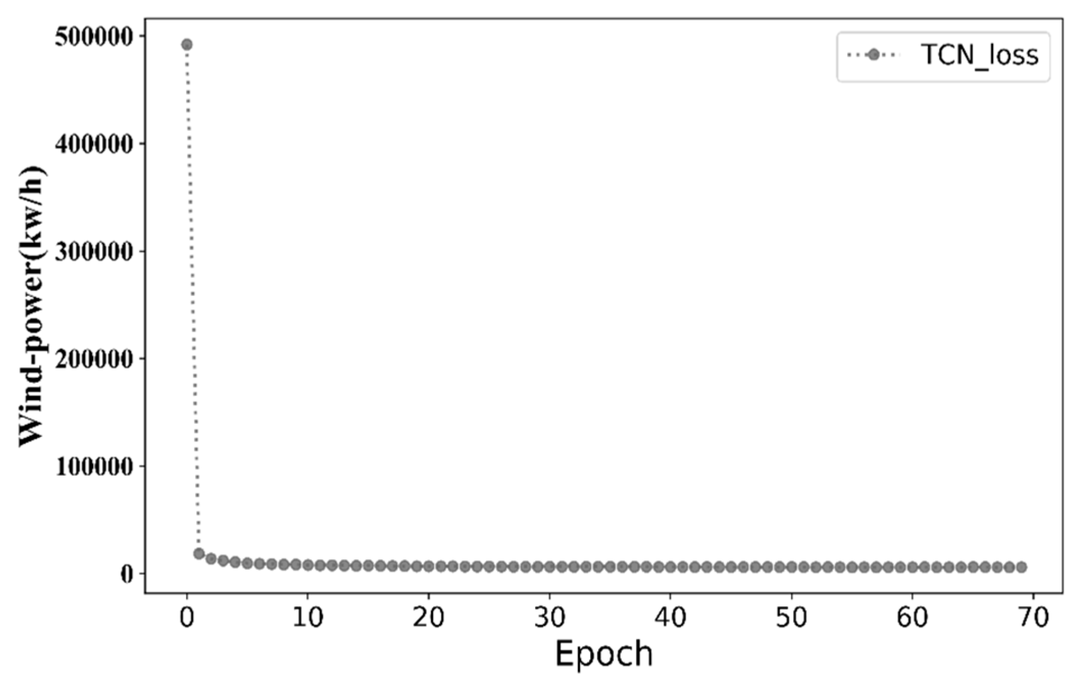
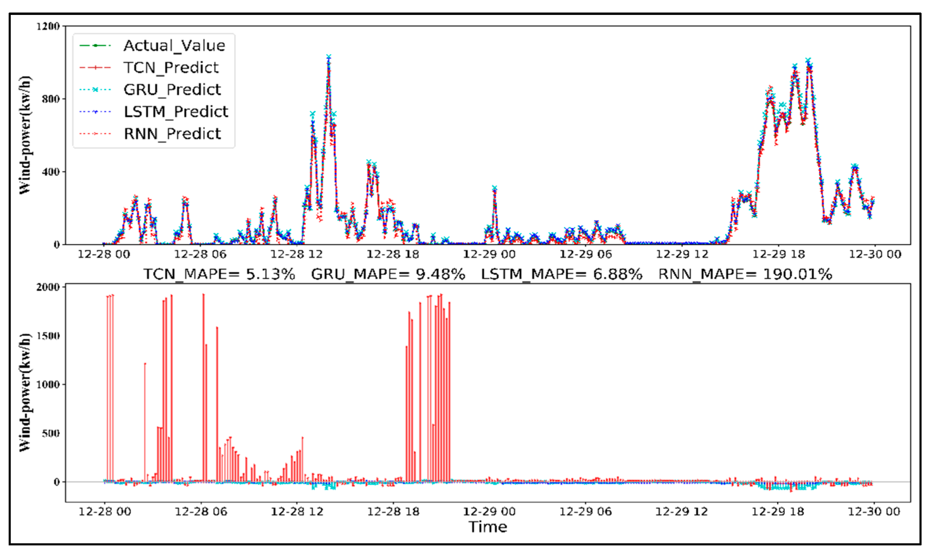
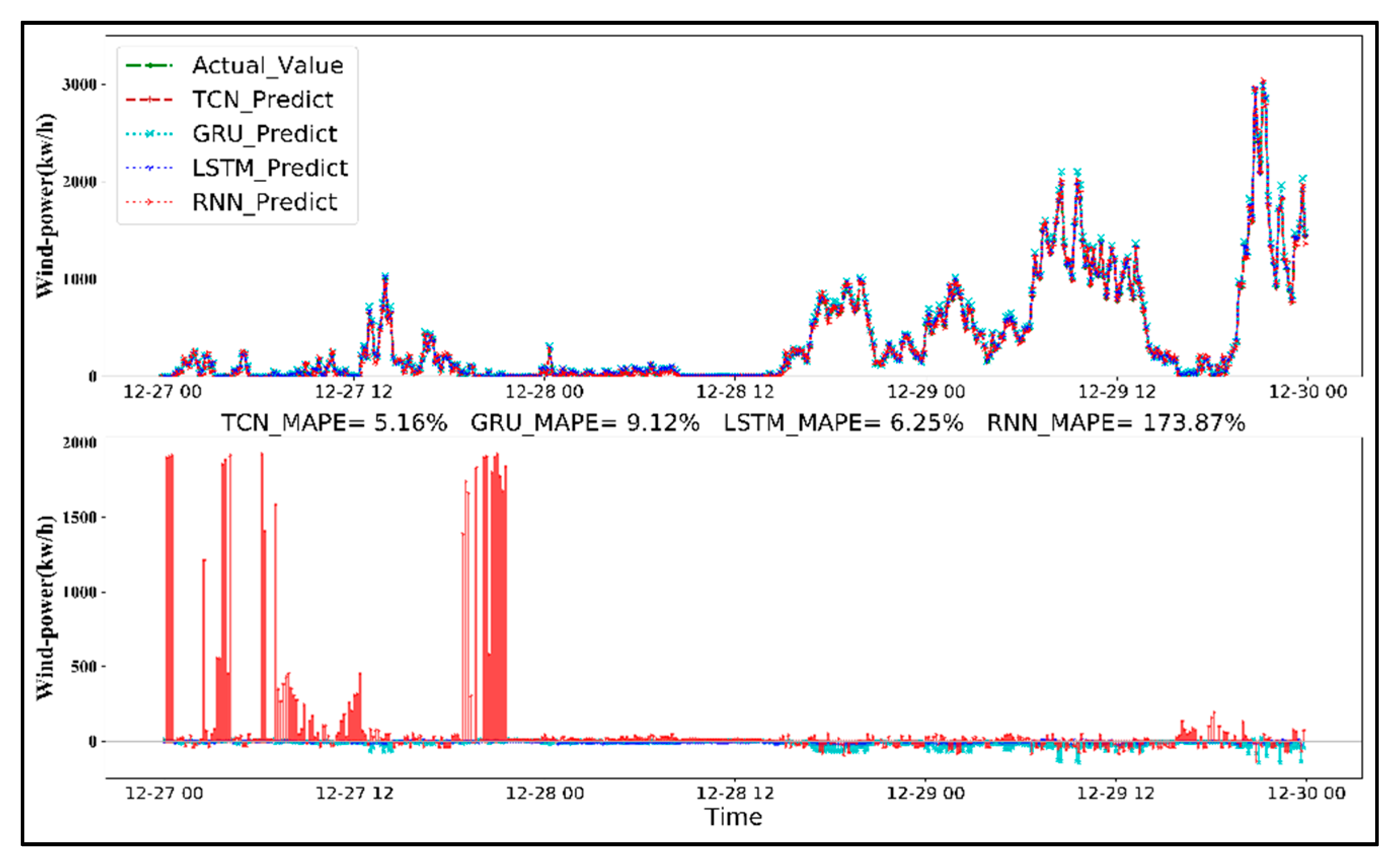
In our experiment, the prediction error of the TCN model for wind power prediction decreased most steadily among the four models, followed by LSTM, GRU, and RNN.

▪

With an increasing amount of historical data, the prediction error (MAPE) of the TCN-based model decreased significantly; the 72 h forecast error of the 1-week, 1-month, and 1-year training datasets was 66.43%, 10.93%, and 5.13%, respectively.

▪

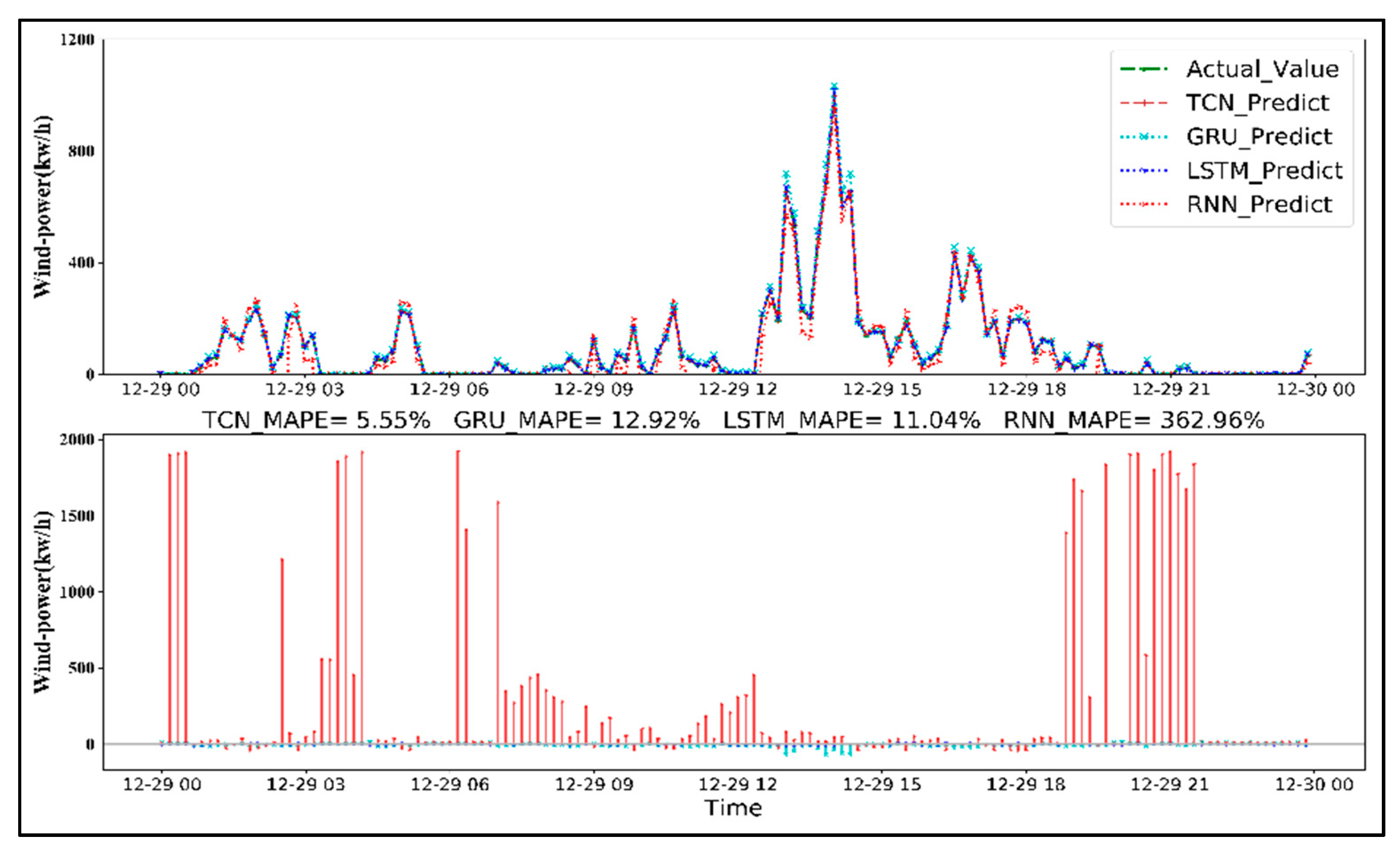
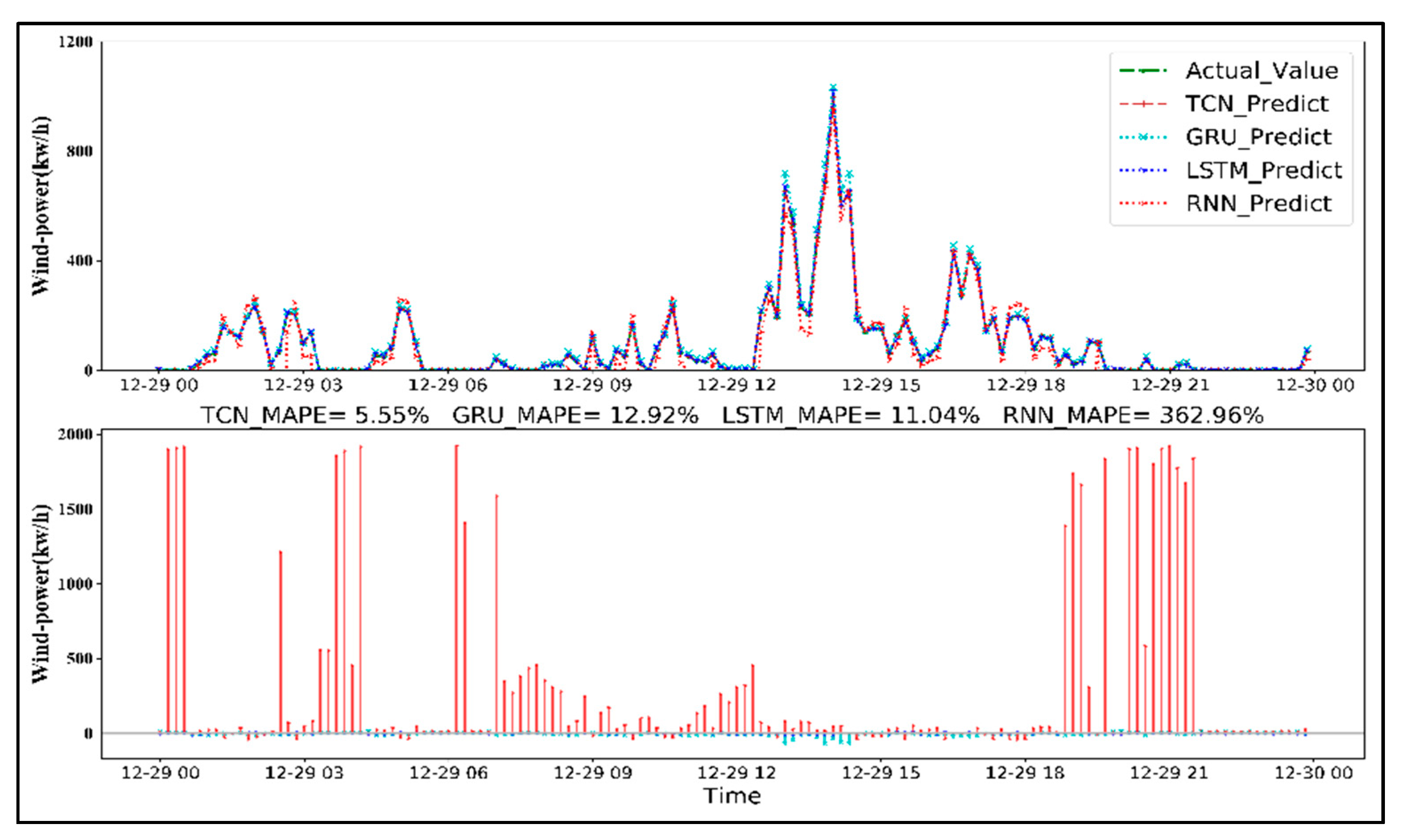
Compared with LSTM, GRU, and RNN models, the TCN model created long effective memory in the deep learning framework and exhibited a lower forecast error to predict 24-, 48-, and 72-h ahead of wind power generation, which is more suitable for sequence modeling based on sequence-to-sequence applications.

The remainder of this article is organized as follows. Section 2 provides a review of other relevant studies in this field, and Section 3 introduces the proposed TCN-based model for wind power forecasting. The results and performance analysis are presented in Section 4. Finally, Section 5 provides the concluding remarks.

2. Literature Review

This section provides an overview of deep neural networks (DNNs) in relation to their processing of time-series data and the application of the differential evolution (DE) algorithm to improve the forecast accuracy of wind power generation.

2.1. DNNs for Processing Time-Series Data

To address the issues involved in wind power forecasting, researchers have developed DNNs, which include the RNN, LSTM, GRU, and TCN and can be applied to address complex nonlinear relations between wind power output and climate data.

RNNs can manage several types of sequence problems, including speech and text recognition, language-to-language translation, handwriting recognition, and sequence data analysis (i.e., forecasting). Generally, RNNs are the best candidate for sequence-to-sequence learning because their internal memory gates obtain outstanding results in natural language processing and other applications. However, RNNs have limited testing with wind time-series data, as well as long memory requirements. LSTMs were later designed to avoid the vanishing gradient that occurs with long sequences. A simplified version of the LSTM, the GRU was applied to resolve simple problems using shorter sequences. In 2016, Lea et al. [20] first proposed temporal convolutional networks (TCNs) for video-based action segmentation. In practice, TCNs have all the advantages of LSTMs as well as extended memory processing input based on dilated convolution architecture and residual connections, with higher classification accuracy than LSTMs.

TCN architecture is based on dilated casual convolutions that enable an exponentially large receptive field. This is more suitable for sequence modeling based on sequence-to-sequence applications that require long effective memory, such as long- or medium-term wind power forecasting [14]. Dilated convolution is a means of increasing the receptive view of the network exponentially, as well as linear parameter accretion [21]. Thus, TCNs are considered a better-adapted architectures thanks to their simplicity, autoregressive prediction, and flexibility for sequence modeling, with a large long memory.

Many researchers have demonstrated that TCNs effectively perform sequence-to-sequence tasks, such as machine translation or speech synthesis in text-to-speech systems. Bai [21] conducted a systematic evaluation of generic convolutional and recurrent networks for sequence modeling and reported that the TCN outperformed canonical recurrent networks across a broad range of standard tasks. Four deep learning network schemes for wind power forecasting are summarised in

Table 2. Deep Learning Approaches for Wind Power Forecasting.

	Features	Limitations
RNN [14]	Used for mapping inputs to outputs of varying types and lengths, and are fairly generalized in their applications such as text translation and voice recognition.	RNNs have a major setback called the exploding/vanishing gradient, which causes difficulties in learning long-range dependencies. RNNs become severely difficult to train as the number of parameters becomes extremely large.
LSTM [15,16]	LSTMs are a novel, efficient, gradient-based method for handling complex, artificial long-time-lag tasks. Essentially, LSTMs are a special kind of RNN capable of learning long-term dependencies.	LSTMs require a lot of memories and time in order to be trained for real-world applications. LSTMs can solve the problem of vanishing gradients; however, they fail to remove it completely.
GRU [17,18,19]	GRUs reduce the number of gating units on the LSTM model and optimize the network structure, which is now widely used in industrial practice.	GRU models have problems with slow convergence rate and low learning efficiency, resulting in too long a training time, and even under-fitting.
TCN [20,21,22,23]	TCNs consist of dilated, causal 1D convolutional layers with the same input and output lengths to create a powerful forecasting model in distinct domains.	Many studies show that TCNs exhibit better performance than RNNs in domain applications, while avoiding the drawback of the exploding/vanishing gradient problem in RNN models.

.

TCNs exhibit outstanding behavior with sequences of undetermined length, and the TCN architecture can assist engineers in managing information flows in incredibly long sequences. Consequently, TCNs have stronger learning capabilities and exhibit equal or better results compared to those of the RNN, LSTM, and GRU.

To meet the large memory requirements for DLNs, TCNs use one-dimensional (1D) separable convolutions to factorize a standard convolution into a depth-wise and pointwise convolution. Typically, the TCN consists of three parts: dilated causal convolutions, nonlinear activation, and residual connections. A causal convolutional network is used with 1-dimensional fully convolutional network architecture. A key characteristic is that the output at time t is only convolved with the elements that occurred before t. In 2020, Yan et al. [23] used a TCN for weather state predictions in a comparative experiment conducted with an LSTM. Notably, the results demonstrated that the TCN outperformed other models, including the RNN, LSTN, and GRU, in prediction tasks with time-series data. As shown in Figure 1, the TCN used the 1-dimensional convolutional neural network for short-term wind power prediction, showing that it not only retained the powerful ability of feature learning from both the weather data and electric power output, but was also suitable for processing large volumes of time series data.

2.2. Differential Evolution Algorithm

In the design of DNNs for processing time-series data, the optimal parameters of the developed model are identified from training data in order to achieve high predictive precision in the model output.

In supervised machine learning algorithms, in order to minimize the convergence loss of the model in the learning process the optimal parameters of the model can be investigated using evolutionary algorithms (EAs). Practically, the EA algorithm is an effective and efficient approach for solving global numerical optimization problems, avoiding overfitting, and preventing the gradient descent algorithms from converging prematurely on a local suboptimal solution. EAs constitute a smart approach to solving constrained multiobjective optimization problems. In practice, EAs are a family of nature-inspired algorithms widely used for solving complex optimization problems which can be used for assisting developers in determining the optimal parameters of the training model. The differential evolution (DE) algorithm [24,25,26,27,28] is a branch of EA that follows the general procedures of EAs.

In detail, DE is a metaheuristic method that optimizes a problem by iteratively attempting to provide an improved candidate solution with regard to a set measure of quality. DE was introduced by Storn and Price in the 1990s [16], and is applied to solve multiobjective optimization with constraints. Typically, metaheuristic methods can search large spaces for candidate solutions. DE is particularly used for multidimensional real-valued functions; however, it does not use the gradient of the problem being optimized and therefore does not require the optimization problem to be differentiable. Thus, DE can be used on optimization problems that are not continuous, noisy, or changeable over time.

The three basic operators of the DE algorithm are the mutation, crossover, and selection operators. The fundamental idea behind DE is a scheme for producing trial vectors according to the manipulation of target vector and difference vector. If the trail vector yields a lower objective function than a predetermined population member, the newly generated trail vector will replace the vector and be compared in the following generation [28].

After the initialization process, DE forms a loop of the mutation, crossover, and selection processes until the termination condition is satisfied [24]. The processes of these operators are described as follows:

(i)

Initialization

Suppose that each individual of the population is denoted as X_i = [x_ij] = (x_i,1, …, x_i,j, …, x_i,D), where i = 1, …, N, N is the number of the solution as well as j = 1, …, D, and D represents the number of the dimension. X_i is limited by X_min = ($x_{min}^G$, …, $x_{min}^G$, …, $x_{min}^G$) and X_max = ($x_{max}^G$, …, $x_{max}^G$, …, $x_{max}^G$), which is specified by the user. G is the generation number.

An individual of the population can be defined as follows:

X_i = (x_i,1, …, x_i,j, …, x_i,D), i = 1, …, N. j = 1, …, D

(1)

First, the initialization population randomly selects the initial parameter values uniformly based on the intervals [X_min, X_max]. The commonly used initialization method for individuals is

$$X_i^G=rand\left(0,1\right)·\left(X_{max}-X_{\min }\right)+X_{min}$$

(2)

where rand(0, 1) represents the generation of a uniformly distribution random number located in [0, 1].

(ii)

Mutation

The DE algorithm adopts the mutation strategy, in which a mutant vector is created for each individual $V_i^G$ (also called the trial vector) in each generation G. For a given parameter vector $V_i^G$, three vectors are selected randomly: $X_{r1}^G$, $X_{r2}^G$, and $X_{r3}^G$, such that the indices i, r₁, r₂, and r₃ are distinct. First, the weighted difference of two of the vectors is added to form$V_i^G$

$$V_i^G=X_{r1}^G+F·\left(X_{r2}^G-X_{r3}^G\right),$$

(3)

where F is the scaling factor that controls the amplification of the differential evolution, i.e., mutation scale; its value is located in [0, 2]. Small values of F will lead to smaller mutation step sizes. Consequently, it will take longer for the algorithm to converge. Conversely, large values of F enable exploration, but can lead to the algorithm overshooting good optima. Thus, the value has to be small enough to enhance local exploration but also large enough to maintain diversity [25]. A well-known DE mutation operation is described as follows [26,27]:

$$V_i^G=V_{best}^G+F·\left(V_{r1}^G-V_{r2}^G\right)$$

(4)

$$V_i^G=V_{r1}^G+F·\left(V_{r2}^G-V_{r3}^G\right)+F·\left(V_{r4}^G-V_{r5}^G\right)$$

(5)

$$V_i^G=V_i^G+F·\left(V_{r1}^G-V_{ri}^G\right)+F·\left(V_{r2}^G-V_{r3}^G\right),$$

(6)

where r₁, r₂, r₃, r₄, and r₅ are the distinct integers randomly generated from the range of [1, N] and are not equal to i, i.e., (r₁ ≠ r₂ ≠ r₃ ≠ r₄ ≠ r₅ ≠ i). $V_{best}^G$ is the best individual with the highest fitness value (objective value) at generation G.

(iii)

Crossover

After mutation, a trial vector $X_i^G$ = ($X_{i,1}^G,X_{i,2}^G,\dots ,X_{i,D}^G$) is generated for each individual according to a binomial crossover operator on $X_i^G$ and $V_i^G$, as follows:

$$U_{i,j}^G=\{\begin{array}{cc}{V}_{i,j}^G& if \left(ran{d}_{i,j}\left(0,1\right)\le CR or j==j_{rand}\right)\\ X_{i,j}^G& otherwise\end{array}$$

(7)

In this equation, rand is a uniformly distributed random integer in the range of [1, D], which is generated for each individual. CR is the crossover rate, which is restricted in the range of [0, 1]. CR controls the number of elements that will adjust. Larger values of CR will lead to deriving more variation in the new population, therefore increasing it also increases exploration [25].

If the j-th variable $U_{i,j}^G$ of the trial vector $U_i^G$ violates the boundary constraints, it is reset as follows:

$$U_{i,j}^G=X_j^{min}+rand\left(0,1\right)·\left(X_j^{max}-X_j^{min}\right).$$

(8)

(iv)

Selection

The selection operator determines whether the target or trial vector survives and enters the next generation based on their fitness values. For a minimization problem, the decision vector with the lower fitness value (objective value) can enter the next generation, which can be expressed as follows:

$$X_i^{G+1}=\{\begin{array}{cc}{V}_i^G& if (fit\left(U_i^G\right)\le fit\left(X_i^G\right)\\ X_i^G& otherwise\end{array}$$

(9)

The process is repeated with the expectation, though it is not guaranteed, that a satisfactory solution will eventually be discovered.

3. Wind Power Forecasting Model with Temporal Convolutional Networks

In this section, a TCN-based approach for a long-term wind power forecasting model is presented. A detailed workflow of the TCN model design for 24–72 h wind power forecasting is described herein. The following three subphases comprise the TCN model development process with DE for determining the optimal parameters of the proposed model: (i) architecture design, (ii) determination of the architecture parameters of the model, and (iii) the overall process for model development.

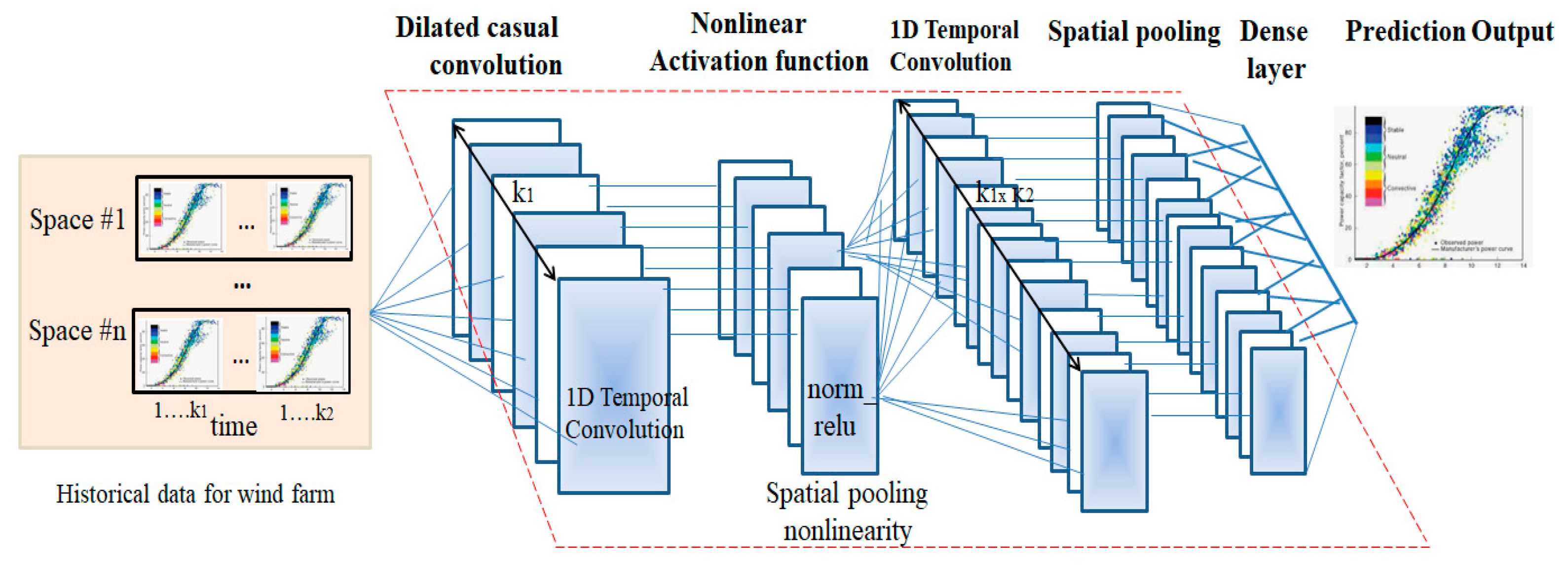
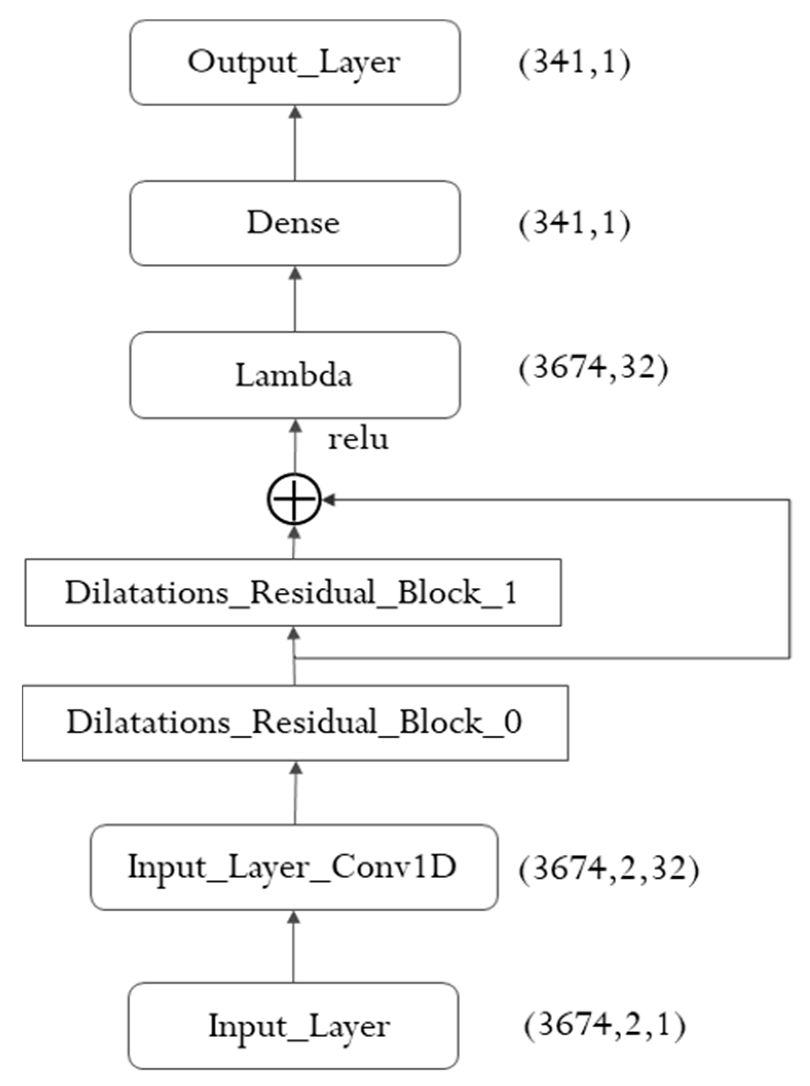
3.1. Architectural Design for TCN

Inspired by [20], we incorporated the convolutional network architecture involved in casual convolution with residual connections to construct a stable TCN-based prediction model for 24–72 h wind power forecasting. Dilated convolution is used to select which values of the neurons from the previous layer contribute to those in the next layer. Thus, the dilated convolution operation captures both local and temporal information.

The dilated convolution function, F(s), is provided by [21]

$$F\left(s\right)=\left(x{\ast }_{d}f\right)\left(s\right)={{\displaystyle \sum }}_{i=0}^{k-1}f\left(i\right)·x_{s-d.i},$$

(10)

where $x_s$ is the current input sequence data at time t, d is the dilation factor parameter, and f is a filter of size k.

The TCN model can be defined as follows [23]:

$$x_t^l=\sigma (W_x^l·F_d\left(x_t^{l-1}\right)+b_x^l+x_t^{l-1}),$$

(11)

where F_d$(.)$ is the dilated convolution function of d factor, $x_t^l$ is the value of the neuron of the l-th layer at time t, $W_x^l$ and $b_x^l$ are the weights and bias corresponding to the l-th layer, and σ is the activation function. The dilated residual block in our project is detailed in Figure 2.

The system must use the residual block to the convolutional layers when deep and large TCNs are employed in order to achieve further stabilization. As presented in Figure 3, the residual connections constituted the addition of the data input to the output before applying the activation function; the residual block (d = 16) is used between each layer in the TCN to accelerate convergence and enable the training of deeper models.

3.2. Parameter Selection for TCN Model Using Evolutionary Algorithm

The architecture design for TCN and optimal parameters for the developed wind power prediction model with the DE search mechanism are analyzed in this section.

3.2.1. Preliminary Architecture Design

In this step, four crucial architecture parameters were selected by transferring learning cases in the TCN predictor [20,21,22,23]; the original parameters of TCN models developed for wind power prediction models were obtained from P. Rémy at GitHub [29], namely, (i) number of filters, (ii) activation function, (iii) optimizer, and iv) dilatation coefficient, in order to decide the initial model architecture for model training.

(i)

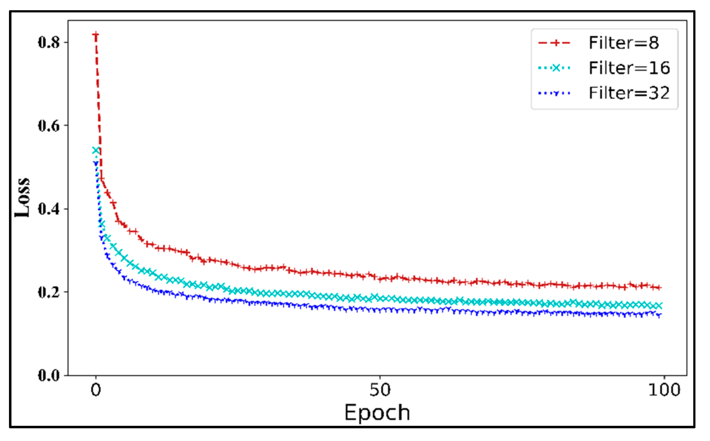
Filter size

In practice, the cost function is a measure of the inaccuracy of the model in terms of the difference between predicted values and real measured values. Following the analysis of three filter sizes (8, 16, and 32), as described in Figure 4, the filter size of 32 exhibited the smallest convergence error of the cost function after 100 iterations of simulation and was the optimal choice for the designed TCN-based prediction model.

(ii)

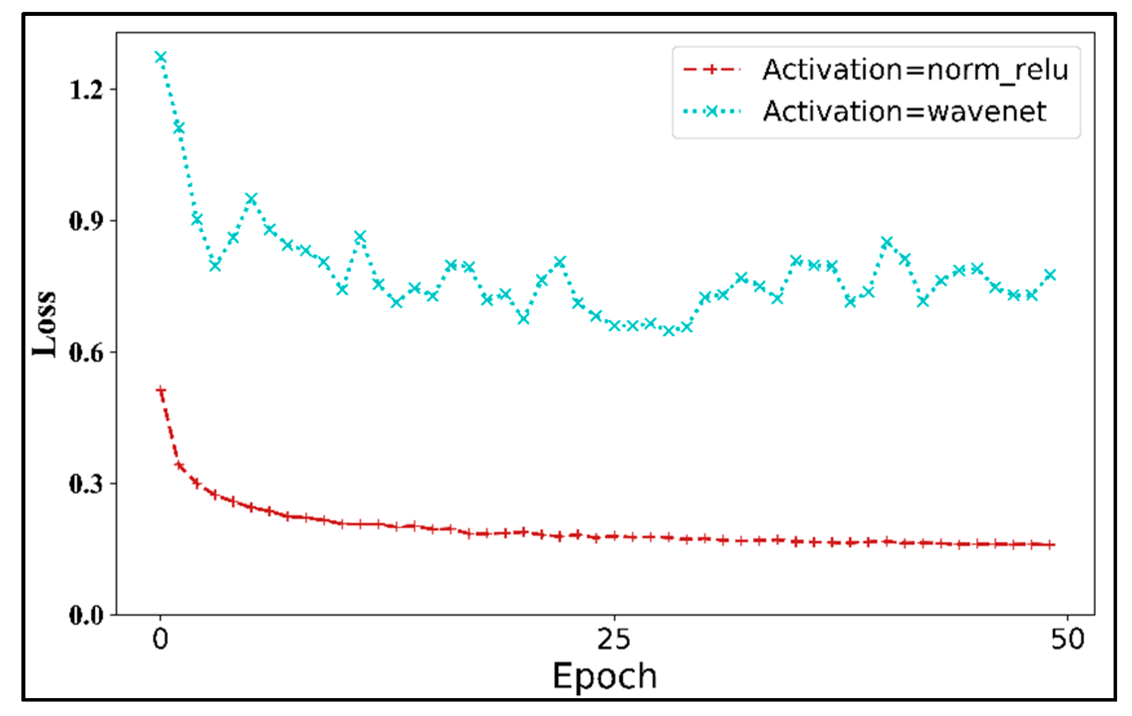
Activation function

In artificial neural networks, the activation function of a node defines the output of that node based on the input or set of inputs. Generally, nonlinear activation functions allow such networks to compute complex problems using a few nodes. In the experiment, we analyzed two types of nonlinear activation function, the norm_relu and Tanh*Sigmoid activation function used in WaveNet. The corresponding convergence error of the cost function for these activation functions is presented in Figure 5; norm_relu was selected as the activation function of the model.

(iii)

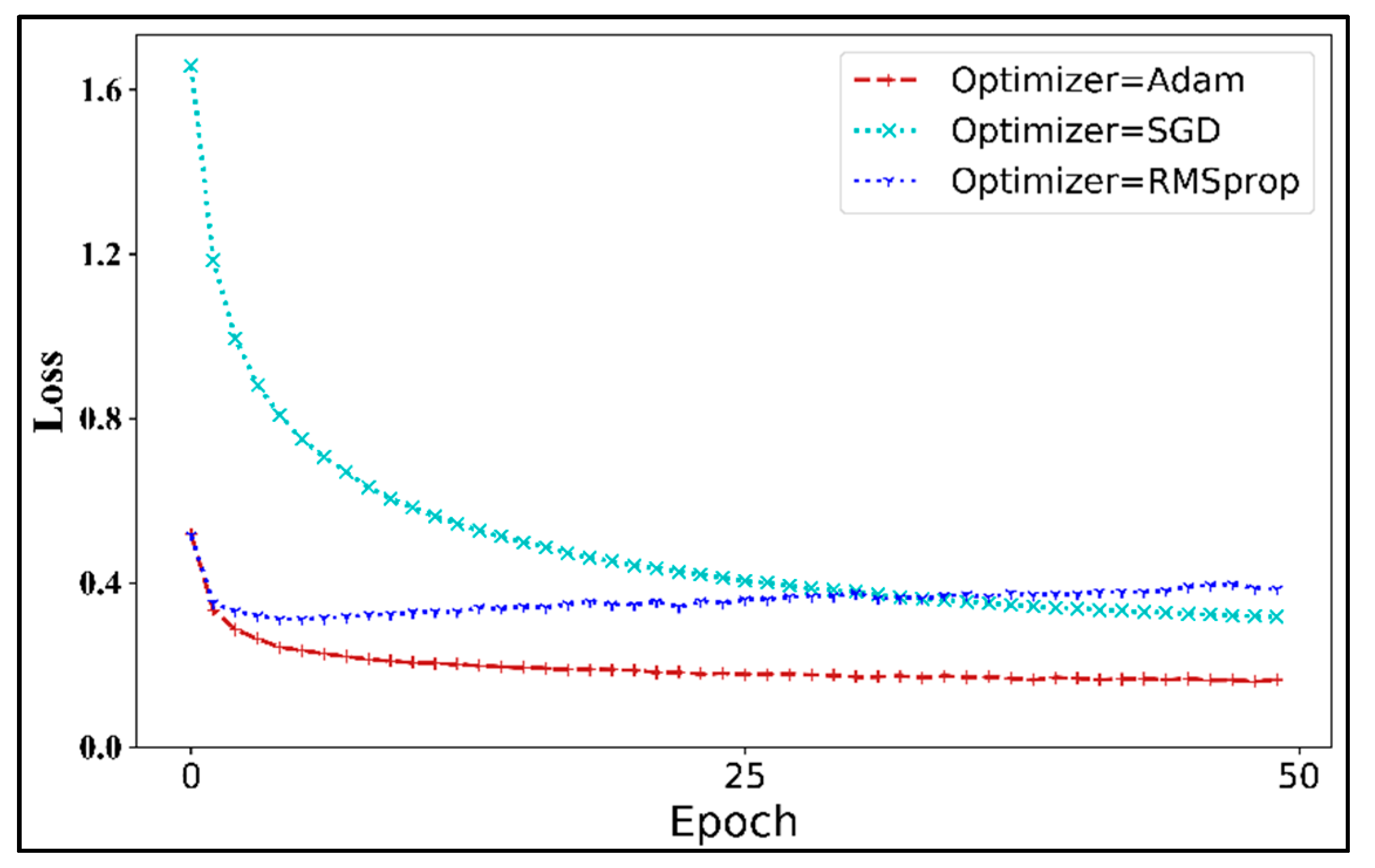
Optimizer

To minimize loss during model training, an optimizer was adopted to improve the accuracy of the model through adjustment of the filter weights. We assessed three popular optimizers in the TCN model, Adam, SGD, and RMSprop; the corresponding convergence error of cost function is detailed in Figure 6. The Adam optimizer was chosen as the ideal optimizer for model training.

(iv)

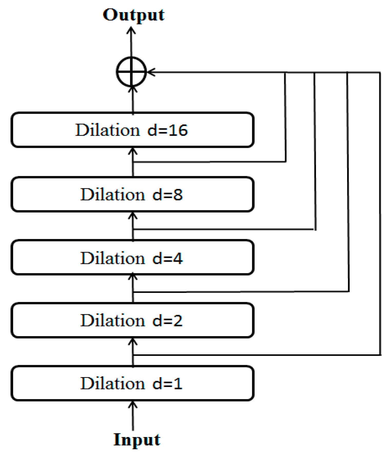
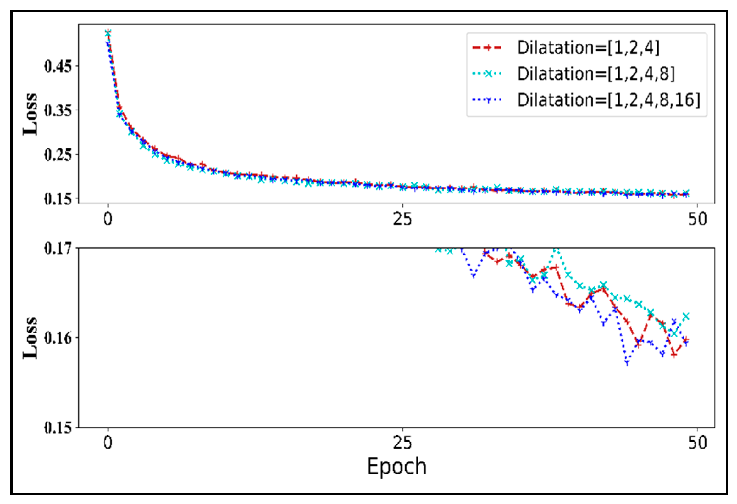
Dilatation coefficient

Following the analysis of three combinations of dilatation coefficients (1, 2, 4; 1, 2, 4, 8; 1, 2, 4, 8, 16) in the model input architecture, the third set (1, 2, 4, 8,16) achieved the most optimal results in relation to the error convergence of the cost function, as depicted in Figure 7.

The architectural components of the proposed TCN model for transferring learning from model training are listed in

Table 3. Architecture of the proposed TCN model.

	Number of Filter	Kernel_Size	Dilatations	Number of Stack	Optimizer
Parameter Value	32	10	[1, 2, 4, 8, 16]	2	Adam

.

To confirm the appropriate architecture of the model design, different model architecture parameters were experimentally investigated. In this experiment, 83.3% (500,000 records) of the data from the open dataset of wind farm in Turkey (2018) [30] was randomly selected to serve as the training dataset, and the remaining 17.7% (100,000 records) was used for testing. The average accuracy of the results of experimental training and testing is summarized in

Table 4. Accuracy analysis of the TCN model architecture.

	Maximum	Minimum	Average
Training accuracy	98.2%	97.1%	97.8%
Test accuracy	96.7%	92.9%	95.1%
Average	97.45%	95.0%	96.4%

. Model accuracy was above 96.4% based on different parameter combinations, with a low convergence loss result for the cost function. Thus, the architectural parameters of Table 3 for the TCN model were validated.

3.2.2. Analysis of Architecture Design

Following the architecture analysis step of detailed model design, experiments were conducted with model training in order to validate the optimal parameters of the developed TCN model based on training samples. In the experiment, differential evolution (DE) methods [24,25,26,27,28] explored these solutions to handle the hyper-parameter tuning of the TCN model for predicting wind power output in order to reach the satisfactory prediction accuracy for different weather conditions. Essentially, the DE method is a population-based stochastic search process using the distance and direction information from the current population to conduct its search. Inspired by [25], we selected the DE method to solve our problem because the historical data for wind power generation are generally not continuous, noisy, or changeable over time; thus, the gradient of the problem being optimized is not used.

For all experiments, 50 independent runs were conducted for each test function. The parameter settings for the DE algorithm are listed in

Table 5. The parameter settings for the architectural analysis.

Algorithm	Parameter Setting
DE	NP = 10, F = 0.5, CR = 0.3, G = 30

. As shown in Table 5, the following parameters were chosen for the application of DE: population size NP = 10; scaling_rate F = 0.5, crossover_rate CR = 0.3, generation number G = 30, and maximum iteration = 500. Optimization was terminated at the pre-specified number of generations.

Then, nine trial vectors $V_i^G$ and difference vectors (

Table 6. The parameter settings for the nine trial vectors.

Target Vector	Filter_Size	Dilatation	Number of Stacks	Activation Function	Optimizer
#1	8	[1, 2, 4, 8]	2	norm_relu	RMSporp
#2	32	[1, 2, 4, 8, 16]	2	wavenet	RMSporp
#3	16	[1, 2, 4, 8]	4	norm_relu	Adam
#4	8	[1, 2, 4, 8]	3	norm_relu	SGD
#5	32	[1, 2, 4, 8]	3	wavenet	RMSporp
#6	8	[1, 2, 4, 8]	2	wavenet	SGD
#7	16	[1, 2, 4, 8, 16]	3	norm_relu	SGD
#8	16	[1, 2, 4, 8]	2	wavenet	SGD
#9	32	[1, 2, 4]	4	norm_relu	Adam

) were generated for each generation G according to the mutation, crossover and selection operations using Equations (1)–(9). If the trail vector yielded a lower error value of objective function than a predetermined population member, the newly generated trail vector replaced the target vector and was compared in the following generation.

For analysis of the optimal parameters of the TCN model, DE allows for the process of mutation, crossover, and selection until the termination condition is satisfied, using Equations (1)–(9); the analysis process is shown in Figure 8.

In our experiment, the error value and error reduction speed of the loss function were adopted to evaluate whether the appropriate model parameters had been selected. If the convergence error decrease was not smooth (i.e., a bouncing phenomenon), the cost function or model parameters required adjustment. The convergence error of cost function in the training process for TCN model is illustrated in Figure 9.

As shown in Figure 9, a stable convergence was reached after a stable error descent was exhibited in the experiments. Overall, the experimental results for the selected optimal parameters of the TCN model are listed in

Table 7. Selected optimal parameters of the TCN model.

Algorithm	Layers	Total Params/Kernels	AF/LF	Optimizer	Dilations	Number of Stack
TCN model for wind power prediction	TCN	45,761/16	norm_Relu	Adam	[1, 2, 4, 8]	4
	Input Layer	0	-
	Initial_Conv	(11,16)
	Dilated ConvLayer	(16,161,16)	norm_Relu/MSE
	Dropout layer	0
	Conv Layer	(16,17,16)	norm_Relu/MSE
	OutputDense Layer	(17,1)	linear

AF = activation function, LF = loss function, MSE = mean squared error.

.

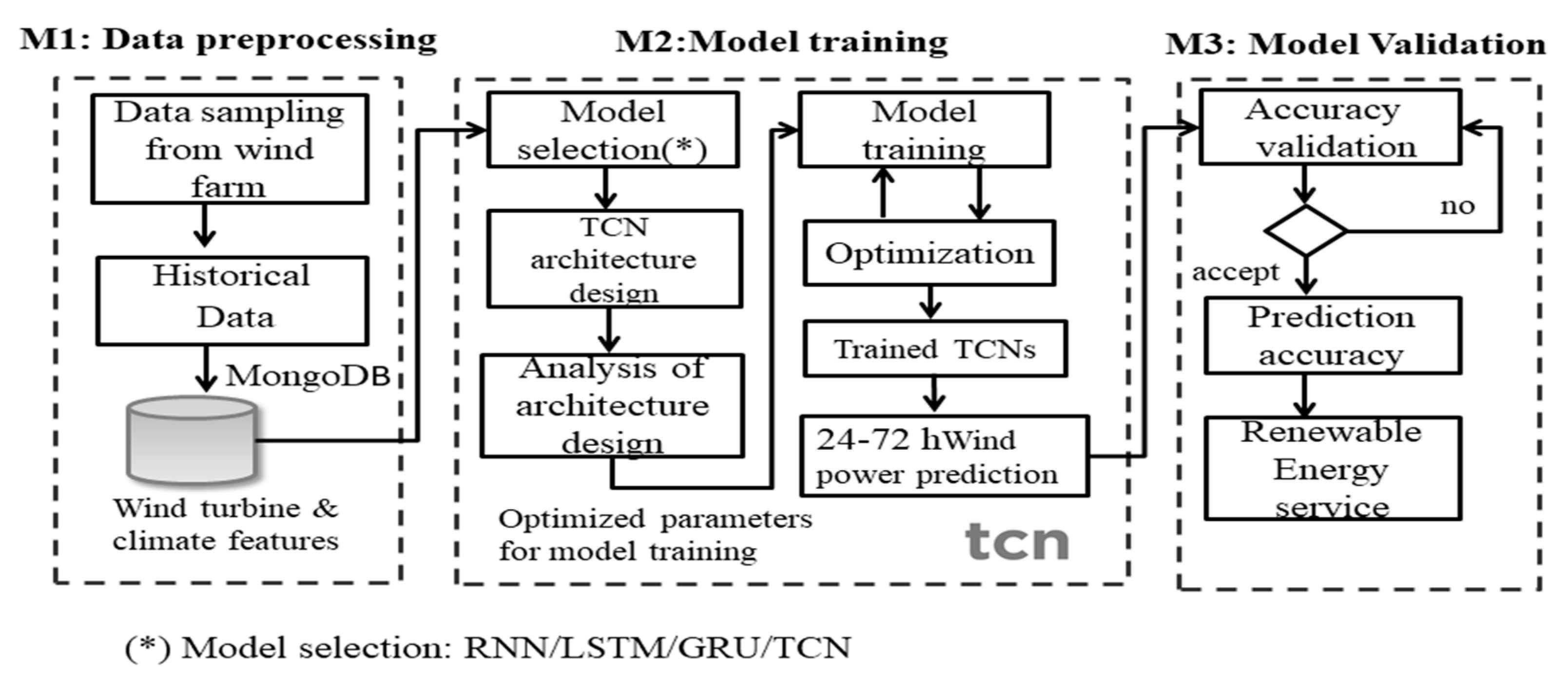
3.3. Overall Process of the Model Operations

Four experimental DNN models for wind power forecasting incorporating RNN, LSTM, GRU, and TCN were employed to verify the performance of model training. The execution process of model development is illustrated in Figure 10. The proposed TCN model comprised the following three subphases in the model operation process: (i) data preprocessing, (ii) model training, and (iii) model validation.

Step 1. Data preprocessing

Before performing model pretraining, engineers must perform data processing for wind farm datasets that contain real weather observations and wind turbine power outputs with anomaly data. Each record in the wind power dataset includes items such as wind speed, wind direction, temperature, humidity, height of wind turbine for model pretraining, and some null fields where linear proportions of the neighbouring observation data are noted in advance.

Following the study of patterns in high-dimension data using principal component analysis, the prediction experiment employed two key model parameters, wind speed and wind direction, which were applied to model training.

Step 2. Model training

Step 2.1 Model pretraining

In the pretraining phase, the proposed model incorporated the gradient descent optimization algorithm in order to fine-tune the model parameters for transfer learning using error derivatives of back-propagation with the optimizer for all layers. Then, a series of experiments were pretrained to investigate the performance of the TCN-based classifier using the Scada dataset, where the learning results were regarded as a basis of the optimal model parameters, including number of filters, dilatation coefficient, activation function, epochs, and prediction accuracy (Table 2).

Step 2.2 Model fine-tuning

During the fine-tuning of the model, we adopted a cross-validation scheme to evaluate the predicted accuracy of the model and overcome the problem of over-training using various n-folds of the cross-validation scheme. For example, k = 5 indicates that 80% of the dataset collected was used in the training experiment, with the remaining 20% used for alternative testing that was repeated five times. In the model validation phase, the system provided a quick response for wind power forecasting using the weights of the neural nets employed in the trained TCN model learning.

Step 3. Model validation

To test the robustness of the proposed model, the trained TCN model associated with the test dataset was adopted to examine the model performance. Finally, the MAPE was selected to evaluate the power prediction performance of the proposed model as follows:

$$MAPE=\frac{1}{n}{{\displaystyle \sum }}_{i=1}^n\left|\frac{O_i-\widehat{O_i}}{W_i}\right|,$$

(12)

where $W_i$ represents the installed capacity of the wind turbine, $O_i$ is the real value, and $\widehat{O_i}$ is estimated output.

In the experiment, an open historical dataset from the Scada wind farm in Turkey, including real weather observations and wind turbine power outputs, was used in model pretraining. Each record of the Scada dataset can be found in [30].

The detailed algorithm for wind power prediction with the TCN-based model is described by PDL as follows (Algorithm 1).

Algorithm 1 Pseudocode of the TCN-based model for wind power prediction.

Input: 1. Historical weather data and wind turbine power outputs from Scada wind farm in Turkey, containing five parameters sampled every 10 min, with a total of 52,560 samples listed. 2. Model parameters of the proposed TCN model including the batch set, kernel, and epochs.

Output: predicted accuracy of wind power generation

1: Initialize the model parameters of the model

2: Set the value of the epochs to 50

3: Assign the stop condition value (ε) as 0.0001

4: Training loop

5: While (the number of epochs) do

6: Determine the optimal parameters of TCN model, as given in Equations (1)–(9)

7: Perform the wind power prediction, as given in Equations (10) and (11)

8: Return (model_file)

9: The training results of the model_file include: (1) filter size, (2) activation function, (3) optimizer, (4) dilatation coefficient, (5) final loss of the cost function, and (6) output result of the training process ($\widetilde{O_i}$)

10: Return train (output_file)

11: End loop

12: Test phase

13: Accuracy prediction with loss of cost function by using specific parameters from the model

14: return predict (accuracy)

15: End

4. Results

In this section, the performance of the proposed TCN-based model for wind power prediction is demonstrated by means of an example. The experiments were conducted using the Python programming language and TensorFlow, which is an open source software library for numerical computation. Moreover, TensorFlow incorporates numerical libraries such as Pandas, NumPy, and Matplotlib for computation. The parallelisation of the multicore architecture increased the computation speed of the TCN model. The multicore architecture included an AMD Ryzen Threadripper processor (3.4 GHz) with 32 GB RAM, a 64-bit Ubuntu 14.04 operating system, an Nvidia GeForce GTX 1080 graphics card (GPU), graphics core computing, and the MongoDB 2.2.6 database. The experimental environment is described in

Table 8. Experimental environment for TCN-based prediction model.

IP	Programming Language	Operating System	Numerical Library
192.168.1.10 (AMD Ryzen Threadripper, 1920X, 3.4G)	Python 3.5	Ubuntu 14.04 LTS 64	Tensorflow-gpu 1.1.3
			Pandas 0.23.4
			Numpy 1.1.8
			Matplotlib 3.3.2

.

4.1. Case Study: Performance Analysis for TCN-Based Model (Scada Wind Farm, Turkey)

Step 1. Data preprocessing phase

In the experiment, an open historical dataset from Scada wind farm in Turkey, including real weather observations and wind turbine power outputs, was used in model pretraining. Each record in the Scada dataset contained five parameters sampled every 10 min, with a total of 52,560 samples listed [31]. Notably, some null fields contained linear proportions of the neighbouring observation data in advance. Our training dataset comprised samples from 1 January 2018, to 26 December 2018, and the test dataset used samples from three days, namely December 27 to 29, 2018.

Scada Systems measured and saved data including wind speed, wind direction, generated power, etc. This file was taken from a Scada Systems wind turbine working and generating power in Turkey. The data in the file are listed as follows: [30]

• Date/Time: 10 min intervals
• LV ActivePower (kW): The power generated by the turbine for that moment.
• Wind Speed (m/s): The wind speed at the hub height of the turbine.
• Theoretical Power Curve (KWh): The theoretical power values that the turbine generates with that wind speed, which is given by the turbine manufacturer.
• Wind Direction (°): The wind direction at the hub height of the turbine

Step 2. Model training phase

To examine model efficiency, four deep neural models were incorporated for series data processing, namely, RNN, LSTM, GRU, and TCN, in order to conduct wind power forecasting 72 h ahead of time. We set the initial values of TCN model parameters as in Algorithm 1, and the experiment parameters for the RNN, LSTM and GRU models as in

Table 9. Experimental parameters for RNN, LSTM and GRU prediction models.

	Parameter	Output Unit	Optimizers	Learning Rate (lr)	Layers
Model
RNN		64	RMSporp	0.002	3
LSTM		64	RMSporp	0.002	2
GRU		32	RMSporp	0.01	2

.

Step 3. Model validation phase

Two experiments with training datasets of different sizes (i.e., one month and one year) were conducted to verify the effectiveness of the four DNN-based models for wind power forecasting.

In the first experiment, the one-month dataset was used to train four DNNs. The LSTM model had the lowest prediction error (MAPE = 3.8%), followed by the GRU (9.09%) and the TCN (10.93%) models, with the RNN model exhibiting the poorest performance (11.21%), as detailed in Figure 11.

In the second experiment, the one-year historical data were used to pretrain the four DNNs; the prediction results for 24, 48, and 72 h are presented in Figure 12, Figure 13 and Figure 14. For 72 h ahead of time, the prediction error of the TCN model indicated the highest accuracy (MAPE = 5.13%), followed by the GRU (6.25%), LSTM (9.12%), and RNN (173.87%) models.

4.2. Method Comparisons

Theoretically, the convergence error of the cost function decreased in each iteration of model training, as detailed in Figure 15. As presented in Figure 15, the convergence error gradually converged and decreased with the increasing number of iterations (epochs) when three of the prediction models (TCN, LSTM, and GRU) were applied; the RNN model convergence error did not converge, and the prediction error did not decrease. RNNs are thus not suitable for wind power forecasting from large amounts of temporal–spatial data series inputs. The convergence error of the TCN model decreased more than that of the LSTM close to the twentieth epoch, and continued to decrease steadily with the increasing number of iterations. The prediction error of the TCN model decreased most steadily among the four models, followed by LSTM and then GRU.

The performance of the four prediction models was affected by the varying amounts of input training data. Therefore, performance analysis must be assessed with different amounts of historical data for long-term prediction. In our experiment, different amounts of historical data were used for model pretraining and the output results of the modules were sorted; the stability comparison of the convergence errors is detailed in

Table 10. Performance comparison of four DNN models for wind power forecasting.

	Performance	Excellent	Good	Medium	Bad
Period
Week		RNN	GRU	LSTM	TCN
Month		LSTM	GRU	TCN	RNN
Year		TCN	LSTM	GRU	RNN

. With increasing amounts of historical data, the prediction error (MAPE) of the TCN-based model decreased significantly, and the 72-h forecast error of the one-week, one-month, and one-year training datasets was 66.43%, 10.93%, and 5.13%, respectively. In the experiment, the TCN model exhibited consistent, stable and good prediction results by using selected parameters from the DE algorithm.

In summary, the wind power forecast error (MRE) of the proposed TCN-based model was near 5.13% based on one-year historical data in different climatic scenarios. Compared to the accuracy of other projects in wind power forecasting, the European team’s SafeWind project in 2011 achieved a forecasting error of 17%. In 2017, the predicted error improved to 11%; a project of the BSI electric power company reached within 10% in 2019. As shown in

Table 11. Performance comparison of other real projects for wind power forecasting.

Research Team	Prediction Cycle	Prediction Intervals	Prediction Error (MAPE)
ANEMOS, ANEMOS.plus & SafeWind, 2011 [31]	Short-term	within 36 h	17–35%
ANEMOS.plus & SafeWind, 2017 [12]	Short-term	within 48 h	11–14%
UK Power Networks 2016 [13]	Medium-term	within 120 h	10%
Proposed model	Medium-term	within 72 h	Near 5%

, the proposed TCN-based approach provides a lower prediction error with higher prediction accuracy than those of real projects in studies of wind power forecasting [12,13,31].

5. Conclusions

This study presented a TCN-based model for day-ahead wind power prediction based on a casual convolution architecture with residual connections, in order to learn correlations between meteorological features and wind power generation. The proposed scheme effectively solves the long-distance dependency problem, as demonstrated by the input of large amounts of temporal–spatial series data such as one-year wind power data. The experimental results indicate that TCN models have the capability for feature extraction of long-term sequence data, and exhibit the same or higher prediction accuracy compared to LSTM and GRU models. Overall, the proposed TCN-based approach provides a lower convergence error with higher prediction accuracy than those of other models employed in other studies of wind power forecasting [12,13,31].

References

- Alexiadis, M.; Dokopoulos, P.; Sahsamanoglou, H. Wind speed and power forecasting based on spatial correlation models. IEEE Trans. Energy Convers. 1999, 14, 836–842. [Google Scholar] [CrossRef]
- Cadenas, E.; Rivera, W.; Campos-Amezcua, R.; Heard, C. Wind speed prediction using a univariate ARIMA model and a multivariate NARX model. Energies 2016, 9, 109. [Google Scholar] [CrossRef] [Green Version]
- Mohandes, M.; Halawani, T.; Rehman, S.; Hussain, A.A. Support vector machines for wind speed prediction. Renew. Energy 2004, 29, 939–947. [Google Scholar] [CrossRef]
- Moreno, S.; da Silva, R.G.; Mariani, V.C.; Coelho, L. Multi-step-ahead wind speed forecasting based on a hybrid decomposition method and temporal convolutional networks. Energy 2021, 238, 121981. [Google Scholar] [CrossRef]
- Donadio, L.; Fang, J.; Porté-Agel, F. Numerical weather prediction and artificial neural network coupling for wind energy forecast. Energies 2021, 14, 338. [Google Scholar] [CrossRef]
- Hong, Y.Y.; Rioflorido, C.L.P.P. A hybrid deep learning-based neural network for 24-h ahead wind power forecasting. Appl. Energy 2019, 250, 530–539. [Google Scholar] [CrossRef]
- Mana, M.; Astolfi, D.; Castellani, F.; Meißner, C. Day-ahead wind power forecast through high-resolution mesoscale model: Local computational fluid dynamics versus artificial neural network downscaling. J. Sol. Energy Eng. 2020, 142, 034502. [Google Scholar] [CrossRef]
- Emeksiz, C.; Tan, M. Multi-step wind speed forecasting and Hurst analysis using novel hybrid secondary decomposition approach. Energy 2022, 238, 121764. [Google Scholar] [CrossRef]
- Jiang, P.; Liu, Z.; Niu, X.; Zhang, L. A combined forecasting system based on statistical method, artificial neural networks, and deep learning methods for short-term wind speed forecasting. Energy 2021, 217, 119361. [Google Scholar] [CrossRef]
- Neshat, M.; Nezhad, M.M.; Abbasnejad, E.; Mirjalili, S. A deep learning-based evolutionary model for short-term wind speed forecasting: A case study of the Lillgrund offshore wind farm. Energy Convers. Manag. 2021, 236, 114002. [Google Scholar] [CrossRef]
- Sareta, K. Short-term wind speed forecasting system using deep learning for wind turbine applications. Int. J. Electr. Comput. Eng. 2020, 10, 5779–5784. [Google Scholar]
- Kariniotakis, G. Renewable Energy Forecasting, from Models to Applications; Cambridge Elsevier Science & Technology: Cambridge, UK, 2017. [Google Scholar]
- UK Power Networks. KASM SDRC 9.3: Installation of Forecasting Modules, November 2016. Available online: https://innovation.ukpowernetworks.co.uk/wp-content/uploads/2019/05/Installation-of-forecasting-modules.pdf (accessed on 8 February 2021).
- Gupta, D. Fundamentals of Deep Learning—Introduction to Recurrent Neural Networks. 2019. Available online: https://www.analyticsvidhya.com/blog/2017/12/introduction-to-recurrent-neural-networks/ (accessed on 20 March 2021).
- Hochreiter, S. Long-short term memory. Neural Comput. 1997, 9, 1735–1780. [Google Scholar] [CrossRef] [PubMed]
- Kandpal, A. Generating Text Using an LSTM Network, Codeburst Web Site. 2018. Available online: https://machinelearningmastery.com/text-generation-lstm-recurrent-neural-networks-python-keras/ (accessed on 8 February 2021).
- Firat, O.; Oztekin, I. Learning Deep Temporal Representations for Brain Decoding. In Proceedings of the First International Workshop, MLMMI 2015, Lille, France, 11 July 2015; pp. 25–34. [Google Scholar]
- Ding, L.; Xu, C. TricorNet: A. Hybrid Temporal Convolutional and Recurrent Network for Video Action Segmentation. arXiv 2017, arXiv:1705.07818. [Google Scholar]
- Wang, X.; Xu, J.; Shi, W.; Liu, J. OGRU: An Optimized Gated Recurrent Unit Neural Network. J. Phys. Conf. Ser. 2019, 1325, 012089. [Google Scholar] [CrossRef]
- Lea, C.; Flynn, M.D.; Vidal, R.; Reiter, A.; Hager, G.D. Temporal Convolutional Networks for Action Segmentation and Detection. In Proceedings of the 2017 IEEE Conference on Computer Vision and Pattern Recognition (CVPR), Honolulu, HI, USA, 21–26 July 2017; pp. 1003–1012. [Google Scholar]
- Bai, S.; Kolter, J.Z.; Koltun, V. An Empirical Evaluation of Generic Convolutional and Recurrent Networks for Sequence Modeling. arXiv 2018, arXiv:1803.01271. [Google Scholar]
- Torres, J.F.; Hadjout, D.; Sebaa, A.; Martínez-Álvare, F.Z.; Troncoso, A. Deep Learning for Time Series Forecasting: A Survey. Big Data 2021, 9, 3–21. [Google Scholar] [CrossRef] [PubMed]
- Yan, J.; Mu, L.; Wang, L.; Ranjan, R. Temporal Convolutional Networks for the Advance Prediction of ENSO. Sci. Rep. 2020, 10, 8055. [Google Scholar] [CrossRef]
- Storn, R.; Price, K.V. Differential Evolution: A Simple and Efficient Heuristic for Global Optimization over Continuous Space. J. Glob. Optim. 1997, 11, 341–359. [Google Scholar] [CrossRef]
- Georgioudakis, M.; Plevris, V. A Comparative Study of Differential Evolution Variants in Constrained Structural Optimization. Front. Built Environ. Comput. Methods Struct. Eng. 2020, 6, 1–14. [Google Scholar] [CrossRef]
- Zhang, J.; Sanderson, A.C. JADE: Adaptive Differential Evolution with Optional External Archive. IEEE Trans. Evol. Comput. 2009, 13, 945–958. [Google Scholar] [CrossRef]
- Yu, W.J.; Shen, M.; Chen, W.N.; Zhan, Z.H.; Gong, Y.J.; Lin, Y. Differential Evolution with Two-level Parameter Adaption. IEEE Trans. Cybern. 2014, 44, 1080–1099. [Google Scholar] [CrossRef] [PubMed]
- Li, X.; Yin, M. Application of Differential Evolution Algorithm on Self-Potential Data. PLoS ONE 2012, 7, e51199. [Google Scholar] [CrossRef] [PubMed]
- Rémy, P. Keras-tcn, GitHub. Available online: https://github.com/philipperemy/keras-tcn (accessed on 15 February 2021).
- Erisen, B. Wind Turbine Scada Dataset: 2018 Scada Data of a Wind Turbine in Turkey. Available online: https://www.kaggle.com/berkerisen/wind-turbine-scada-dataset (accessed on 7 January 2021).
- Giebel, G.; Brownsword, R.; Kariniotakis, G.; Denhard, M.; Draxl, C. The State-of-the-Art in Short-Term Prediction of Wind Power: A Literature Overview, 2nd ed. 2011. Available online: http://ecolo.org/documents/documents_in_english/wind-predict-ANEMOS.pdf (accessed on 10 February 2021).