Article

Robust Static Structural System Identification Using Rotations

1
Key Laboratory of Earthquake Engineering and Engineering Vibration, Institute of Engineering Mechanics, China Earthquake Administration, Harbin 150086, China
2
School of Civil and Environmental Engineering, Harbin Institute of Technology, Shenzhen 518055, China
3
Department of Civil Engineering, University of Castilla-La Mancha, 13071 Ciudad Real, Spain
4
Department of Bridge Engineering, Tongji University, Shanghai 200092, China
5
Department of Civil and Environmental Engineering, Universitat Politècnica de Catalunya, BarcelonaTech, 08034 Barcelona, Spain
*
Author to whom correspondence should be addressed.
Appl. Sci. 2021, 11(20), 9695; https://doi.org/10.3390/app11209695
Submission received: 1 September 2021 / Revised: 24 September 2021 / Accepted: 27 September 2021 / Published: 18 October 2021
(This article belongs to the Special Issue Structural Health Monitoring & Nondestructive Testing)

Abstract

:
Deflections are commonly measured in the static structural system identification of structures. Comparatively less attention has been paid to the possibility of measuring rotations for structural system identification purposes, despite the many advantages of using inclinometers, such as a high resolution and being reference free. Although some work using rotations can be found in the literature, this paper, for the very first time, proposes a statistical analysis that justifies the theoretical advantage of measuring rotations. The analytical expressions for the target parameters are obtained via static structural system identification using the constrained observability method first. Combined with the inverse distribution theory, the probability density function of the estimations of the target parameters can be obtained. Comparative studies on a simply supported bridge and a frame structure demonstrate the advantage of measuring rotations regarding the unbiasedness and the extent of variation in the estimations. To achieve robust parameter estimations, four strategies to use redundant rotations are proposed and compared. Numerical verifications on a bridge structure and a high-rise building have shown promising results.

1. Introduction

1.1. Existing Structural System Identification Method

Potential catastrophic events due to the failure or malfunction of civil infrastructures (e.g., bridges, high-rise buildings, dams) might claim people’s lives and cause substantial economic losses. To avoid this undesirable consequence, it is vital to know the current condition of structures. For this reason, structural health monitoring (SHM) and structural system identification have attracted much attention in recent decades [1,2,3]. A basic assumption in structural system identification is that the deterioration or the damage of structures is reflected in the change in structural parameters (such as bending and axial stiffness). These parameters can be estimated by various structural system identification methods using a measured response from structures under external excitations.
Dynamic-based methods account for the majority of structural system identification methods. Depending on the source of excitation, dynamic structural system identification methods are categorized as input–output methods and output-only methods. In the input–output methods, the time history of the excitation and the response are measured to compute frequency response functions. These functions are used to determine the natural frequencies, mode shapes, and damping ratios of the structure using well-established methods [4,5,6]. In the output-only methods [7,8], instead of using heavy, cumbersome and expensive devices to excite large-scale structures in a controlled way, the ambient (wind-induced, traffic-induced and subtle seismic) vibrations are measured conveniently and economically. The modal information of structures can be obtained by analyzing the correlation functions or the spectral density matrices computed from the operating response data. Among these methods, the Bayesian methods [8] can obtain the posterior distributions of the target parameters by combining the assumed distributions of the parameters in the priors and the evidence from the measurements. The error-domain model [9,10,11] can identify parameter values in the existence of systematic errors and detect the presence of unrecognized systematic errors. The residual minimization method [12] can localize model errors and estimate physical parameters by minimizing the force unbalance in the equations of motion.
Compared with dynamic methods, static structural system identification methods are much less developed. Sanayei et al. [13] identified the plate-bending stiffness of a reinforced concrete pier deck with incomplete static test data using accurate forces and displacements. Later, Banan et al. [14] formulated structural system identification as a constrained nonlinear least squares problem by minimizing the discrepancies between the measured and predicted displacements or forces. Hjelmstad et al. [15] incorporated an adaptive parameter grouping strategy with the work from Banan. The proposed method can locate and assess damage even under sparse and noisy measurements. Yang et al. [16] were able to locate and quantify damages in a cantilever beam and two trusses using a flexibility disassembly technique with a baseline model and all DOFs measured. Sun et al. [17] approximated the beam curvatures by the second-order difference of deflections. This work was able to locate damage from the abnormality in the curvature curves while the damage extent could not be quantified.
Recently, observability methods [18,19] were applied in the field of state estimation. This method was able to identify whether a set of available measurements was sufficient to estimate the state of systems. Lozano et al. [20] applied the observability method (OM) to determine the observability of structural parameters in 2D beam models symbolically with static measurements. Later, structural system identification by numerical OM (NOM) was proposed by Nogal [21] to carry out numerical estimation of target parameters. Recently, Tomás et al. [22] and Emadi et al. [23] developed this method to deal with actual measurements on site, including shear deformations. The effects of measurement errors and simulation errors on the estimation accuracy were investigated in [24]. Later, Lei [25] derived the analytical relations that the displacements of beam-like structure should satisfy using OM. The adverse effect of measurement errors on the estimation accuracy was reduced by imposing the compatibility conditions. A new formulation of observability equation with the measurement error terms separated was proposed in [26].

1.2. Application of Inclinometers in Civil Engineering

Existing static structural system identification methods largely measure deflections rather than rotations [16,17,27]. However, wide industrial applications (e.g., automotive, electronics and aviation industries) of inclinometers can be found [28]. The merits of inclinometers make them very desirable for SHM applications [29,30,31,32,33]. Application of inclinometers in SHM of civil structures can be found in the literature; for instance, stadiums Design Plaza Building [34], Tianjin 117 (597 m) [35], construction hoists [36], Lutrive Bridge [32], pavement construction [37], ground movement [38] and slope measurement [39]. In particular, inclinometers are used to reconstruct the deflected shape of bridges due to the difficulty in measuring deflections directly. However, direct use of rotations might be preferred because systematic errors might be introduced into the approximated deflections depending on the assumption made in the basic functions (e.g., precalculated deflected shapes [32], polynomials [40]). Zhang estimated the deflections accurately via the partial least squares method from a Finite Element Model (FEM) without using basis functions [33]. The possibility of locating damage using inclinometers was also investigated in this work. Liu [37] achieved real-time measurement of lift-thickness during highway construction using a system-integrating inclinometer, robotic total station, and laser ranging sensors. Ha et al. [38] developed and applied a wireless MEMS-based borehole inclinometer for automated measurement of ground movement. Hou [41] proposed to monitor interstory drift in building structures via rotation measurements with MEMS inclinometers and an optimized sensor layout. A comparison of inclinometers versus deflection measurements has already been investigated using information entropy metrics [42]. Different metrics to evaluate the goodness of sensor placement were also studied by Papadimitriou [43] and Argyris [44].

1.3. Research Objective

The novelty of this method is that it can determine the observability of target parameters when a measurement set is given. It is highlighted that a systematic procedure to carry out statistical analysis of the distribution of parameter θ using analytical expression is presented. The expression for parameter θ is obtained under the framework of static structural system identification using the observability method. The distribution of the parameters can be determined by the analytical expression from OM and the theory of inverse distribution [45]. The advantage of this method is that it can obtain analytical expression of the target parameters which have clear physical meaning and mathematical elegance. It can avoid the heavy computation burden that normally occurs in the Bayesian method or optimization-based method.
Although inclinometers have been used in SHM for a long time, the research on the use of rotations in structural system identification is very limited. In the case of static structural system identification for beam-like structures [25], it is found that the estimations of bending stiffness were more sensitive to the measurement errors in deflections than errors in rotations using Monte Carlo analysis. However, no theoretical advantage of using rotations can be found. A comparative study of the use of rotations and/or deflections was carried out to justify the theoretical advantage of using rotations over deflections regarding the unbiasedness and the extent of variation in the estimations. Different strategies to use redundant rotations with the aim of improving estimation accuracy are also discussed.
The remainder of this paper is organized as follows. Section 2 describes the algorithm for structural system identification by constrained OM [46], which obtains the analytical expressions for the parameters. Then, the procedure to carry out statistical analysis with the resulting expression is also presented in this section. Section 3 adopts two illustrative examples to justify the theoretical advantages of using rotations over deflections. Section 4 investigates the effectiveness of four strategies to make use of redundant rotations in a high-rise building. Finally, some conclusions are presented in Section 5.

2. Methodology

This section presents the methodology to carry out statistical distribution of the estimations. In Section 2.1, structural system identification using the Constrained Observability Method is introduced. Then, the procedure to carry out the statistical analysis of the distribution of estimations is described in Section 2.2.

2.1. Structural System Identification Using the Constrained Observability Method

In a previous study [20], the observability of structural parameters was determined symbolically by checking the null space of the coefficient matrix of a system of equations adapted from equilibrium equations. The null space for a m × n matrix [A] is the vector space whose vectors satisfy the homogeneous equation as shown in Equation (1).
[ A ] { x } = { 0 }
The null space for matrix [A] is defined in Equation (2).
N u l l ( [ A ] ) = { { x } R n | [ A ] { x } = 0 }
The null space matrix [N] for the matrix [A] is a matrix whose columns form a basis of the null space Null([A]), which can be computed by Gaussian elimination. In fact, any vector in the null space is a linear combination of the basis vectors for Null([A]), i.e., columns of the matrix [N]. In structural system identification using both OM and NOM, the identification of structural parameters is a recursive process in which the parameters that are identified in the last recursive step are incorporated into the input of the current recursive step to enable the identification of other parameters. In each recursive step, the nonlinear variables appearing in the system of equations are treated as linearized ones. However, the assumption of linearity might reduce the number of observable parameters with given measurement sets [39]. Then, two-stage structural system identification using the constrained OM (COM) was proposed. In Stage 1, the original structural system identification using NOM is carried out until no more parameters are observable. In Stage 2, the system of equations from the last recursive step in Stage 1 is reformulated as a constrained optimization problem, minimizing the square sum of the residuals of this system. The procedure to carry out structural system identification using COM is described in the seven steps below, and all the seven steps are the novelty of this method. Stage 1 is related to Steps 2–5, while Stage 2 is related to Step 7.
Step 1: Define an initial FEM using 2D beam elements for the structure to be analyzed. Generate the system of equilibrium equations for this FEM, as shown by Equation (3).
[K]{δ} = {f}
The matrix [K] is the global stiffness matrix that includes the information of length Lj, elastic moduli Ej, area Aj and inertia Ij of element j (j = 1, 2… Ne). The displacement vector {δ} comprises horizontal deflection ui, vertical deflection vi and rotation wi of node i (i = 1, 2… Nn). The force vector {f} comprises horizontal force Hi, vertical force Vi and moment Mi applied on node i (i = 1, 2… Nn). The numbers of elements and nodes in the FEM are denoted by Ne and Nn.
Step 2: Introduce the boundary conditions and values of the increments in displacements and forces during the static test to obtain the observability equations.
The entries in the matrix [K] are sums of monomial ratios, which are the ratios between axial or bending stiffnesses and the square (or cubic) of the length, i.e., E j A j L j , E j I j L j 2 or E j I j L j 3 . In static structural system identification, it is assumed that Lj is known and Ej, Aj and Ij are unknown parameters to be estimated. Note that Ej, Aj, Ij and Lj from different elements might appear in the same entry due to element connectivity. To separate these parameters, each column of matrix [K] is divided into multiple columns such that any resulting column is uniquely related to one monomial (stiffness), EjAj or EjIj. Meanwhile, the displacement vector {δ} is expanded correspondingly. Then, these stiffnesses are extracted from the matrix [K] and the expanded displacement vector is multiplied by them. Hence, a (constant) modified matrix [K*] and a modified vector {δ*} composed of nonlinear products, e.g., EjAjui, EjIjwi, EjIjvi, are obtained, as shown in Equation (4).
[ K * ] { δ * } = { f }
Once the boundary conditions and the forces applied in the non-destructive static test have been defined, it is assumed that a subset of increments in deflections { δ 1 * } of { δ * } are known and a subset of forces {f1} are known, while the remaining parts { δ 0 * } and {f0} are unknown. By static condensation, Equation (4) can be partitioned as Equation (5).
[ K * ] { δ * } = [ K 00 * K 01 * K 10 * K 11 * ] { δ 0 * δ 1 * } = { f 0 f 1 } = { f }
To cluster the unknowns { δ 0 * } and {f0}, Equation (5) can be rewritten equivalently as the observability equation, Equation (6). I and 0 are the null and the identity matrices.
[ B ] { z } = [ K 10 * 0 K 00 * I ] { δ 0 * f 0 } = { f 1 K 11 * δ 1 * K 01 * δ 1 * } = { D }
Step 3: Check the null space matrix [N] of the coefficient matrix [B] to determine the observability of unknowns in {z} and obtain the numerical estimations for observable variables. The structure of the general solution {zg} to Equation (6) is given by Equation (7).
{ z g } = { z p } + { z h } = { δ 0 * f 0 } p + [ N ] { ρ }
{zp} is a particular solution to Equation (6) and {zh} is a solution to the homogeneous version of Equation (6) (i.e., the vector [D] is replaced by zeros). {zh} is a linear combination of the columns of the matrix [N]. The coefficients of the linear combination are denoted by the vector {ρ}. The observability of unknowns in the vector {z} is determined by checking null rows in the matrix [N]. If any row in the matrix [N] is null, then the same row of {zh} is also null. Then, the associated variable in {zg} is determined by the particular solution {zp}. Hence, the variable is uniquely determined and observable. The calculation of the null space matrix [N] should be carried out symbolically to avoid omitting observable variables, because close-to-zero values from numerical calculations might appear in those null rows. The numerical values of the observable variables are obtained from the particular solution of Equation (6) using least squares methods.
Step 4: Check whether new variables in the unknown vector {z} were identified or not. If identified, go to Step 5. Otherwise, go to Step 6.
Step 5: Any identified variables will be incorporated into the preceding input to form the subsequent input and initiate a new recursive step. This may enable the identification of other unknowns in {z}. Steps 2–4 are repeated until no more variables can be identified.
Step 6: Check whether all variables are identified or not. If all the parameters are identified, then end the procedure. Otherwise, go to Step 7.
Step 7: Obtain the estimations of parameters by solving the constrained optimization problem that is adapted from the observability equations in the last recursive step. Since the linearization of the unknowns leads to the reduction in observable unknowns, the nonlinearity in structural system identification is regained by means of solving an optimization problem with the constraints that the linearized products are equal to the product of associated single variables, e.g., EI2v2 = EI2·v2.
Some single variables {zs} may not appear in the unknown vector {z} of Equation (6). A new unknown vector {z*} is obtained by adding {zs} in {z}. A null matrix [] is introduced into the coefficient matrix so that the equations are not violated, as shown in Equation (8).
[ B * ] { z * } = [ B   Ω ] { z z s } = { D }
The objective function (Equation (9)) of the optimization is to minimize the square sum of the residuals (unbalanced nodal forces) in Equation (8).
f ( { z * } ) = i = 1 3 N n ϵ i 2
where ϵi is the residual of the ith equation in Equation (8), and Nn is the number of nodes.
The procedure to carry out structural system identification by COM is summarized in Figure 1.
In stage 1 (Steps 2–5), the observability equations are treated linearly such that the computation is much reduced when compared with nonlinear methods. All the steps in stage 1 are the same as those in structural system identification by NOM. In stage 2 (Step 7), nonlinearity is introduced by imposing constraints via optimization, with the aim of identifying more parameters. As some parameters have been identified in stage 1, the solution space for the optimization algorithm to explore in stage 2 is much reduced, which eases the computation and convergence issues.
It is highlighted that the observability of the parameters can be analyzed in the 7-step procedure. The observability analysis can differentiate the meaningful estimations from those estimations obtained using numerical optimization. That is to say, the numerical estimations from optimization can always provide numerical values for all parameters, but some values are not meaningful as they are not observable due to the limited number or the limited spatial distribution of measurements.

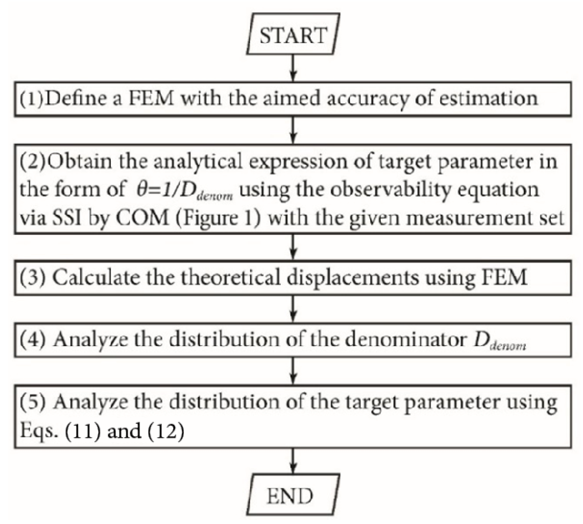
2.2. Procedure for the Statistical Analysis of the Distribution of Estimations

In Step 3 (Figure 1) of the structural system identification using COM described in Section 2.1, instead of obtaining numerical estimations of the variables, the analytical expressions can be obtained symbolically using Gaussian elimination. The obtained analytical expression of the structural parameters is in the form of a fraction with the measurements in the denominator. In this paper, it is assumed that measurement errors follow a normal distribution. Random errors are added to theoretical displacements (usually generated by the FEM) in a proportional manner, as indicated by Equation (10).
δ ˜ = δ r ( 1 + E l e v e l ξ )
where δr is the displacement obtained from FEM and Elevel is the error level; ξ is a random number that follows a normal distribution with zero mean and standard deviation 0.5. The setting of this value is to be consistent with previous research. The effect of choosing such a value is the decrease in the dispersion of the distribution of errors. Hence, it reduces the chance of obtaining more extreme errors.
As the random variables are in the denominator, the definition of inverse distribution is introduced here. Let X be a random variable and the random variable Y be the inverse of X, i.e., Y = 1/X. Then, the distribution of Y is the inverse distribution of X. A closed-form solution for the probability density function (PDF) of the distribution of Y is available when the random variable X follows a normal distribution [45]. If the normally distributed variable X has a mean of µ and standard deviation of σ, i.e., XN(µ,σ2), the PDF of the random variable Y = 1/X (or the inverse distribution of X) is given by Equation (11).
p Y ( y | μ , σ ) = 1 2 π σ y 2 e [ ( 1 y ) μ ] 2 2 σ 2
The distribution of Y is bimodal, and it has a negative mode at y1 and a positive mode at y2.
y 1 = μ + μ 2 + 8 σ 2   4 σ 2   ,   y 2 = μ + μ 2 + 8 σ 2   4 σ 2
The mean and standard deviation for the distribution of Y at a specified interval can be calculated by associated integrations of the PDF pY. These formulas can be found in classic statistic books [45]. With Equations (11) and (12) and the analytical expression of the parameters, the procedure to carry out statistical analysis of the distribution of estimations can be summarized below, and is depicted in Figure 2. Illustrative examples are provided and discussed in detail in Section 3.
  • Step 1: Define a FEM for the structure to be analyzed according to the targeted accuracy of estimations.
  • Step 2: Choose a measurement set to obtain the analytical expression for the target parameter θ, employing structural system identification using COM (see Section 2.1). Rewrite this expression for θ as the reciprocal of an expression denoted by Ddenom, i.e., θ = 1/Ddenom.
  • Step 3: Calculate the theoretical displacements of the structure using the finite element method.
  • Step 4: Analyze the distribution of Ddenom using Equation (10) and the theoretical values obtained in Step 3.
  • Step 5: Analyze the distribution of θ = 1/Ddenom using Equations (11) and (12).
In the parameter estimation problem in power systems, if a measurement set of n measurements is able to identify all the n parameters and the drop in any measurement fails to do so, then this set is defined as an essential set [47]. The availability of analytical expressions for static structural system identification using COM depends on the number and the type of measurements in Step 2. When less than the required measurements, which is equal to the number of unknown parameters, are used, the target parameter is not observable [48]. Neither analytical expressions nor numerical estimations can be obtained. When more than the required measurements are used, the target parameters are observable and can be numerically evaluated, while the analytical expressions are not obtainable. The necessary measurements can be determined by trial and error methods, i.e., adding one measurement each time until the analytical expressions are obtained. It is noted that the trial-and-error method can be carried out using computer programs. However, in the case of a large structure, it could be a heavy workload as there are many combinations of different DOFs. This trial-and-error method certainly can be helped by engineering judgement, which makes the workload much lighter. The measurement sets that are capable of deriving the analytical expressions for the target parameters θ are referred to as essential sets of parameters θ.
In the whole process, MATLAB was used to develop a code based on the procedure in Figure 1 and Figure 2.

3. Theoretical Motivation for Measuring Rotations

The advantages of using rotations are not limited to the practical issues mentioned in Section 1.2. Statistical analyses of two structures were carried out to emphasize the theoretical motivation of measuring rotations rather than deflections. Example 1 corresponds to a simply supported bridge, while example 2 corresponds to a two-story frame.

3.1. Statistical Analysis of a Simply Supported Bridge

Example 1 was a simply supported bridge measuring 3L long. Statistical analysis was carried out for this structure using different measurement sets. The parameterization of the FEM for this structure is shown in Figure 3. The target parameter was EI2. OM (observability method) indicates that any two rotations, or one rotation plus two deflections, or three deflections, in nodes 5–9 are qualified to identify EI2. Without loss of generality, three measurement sets, set 1 (v5, v7, v9), set 2 (v5, v7, w9) and set 3 (w5, w9), were studied, where vi and wi denote the measured deflection and rotation, respectively.
Employing structural system identification using COM with set 3 (w5, w9), the analytical expression of EI2 (as shown in Equation (13)) can be obtained by solving the observability equation symbolically.
E I   2 s e t 3 = L 32 ( w 5 w 9 ) { 16 i = 1 5 ( M i M 14 i ) + 8 M 6 8 M 8 + 4 i = 2 5 [ ( i 1 ) V i L + ( i 1 ) V 14 i L ] + 19 V 6 L + 20 V 7 L + 19 V 8 L }
In Equation (13), the external loads are collected in the numerator while the measurements (w5, w9) are collected in the denominator. The estimation of EI2 depends on the loading case and the measured displacements, not related to EI1 or EI3. Assume that L = 3 m, and the depth and width of the cross section are 0.5 m and 0.3 m. The inertia and the elastic modulus are 3.125 × 10⁻³ m4 and 3.5 × 10⁷ kN/m2, respectively. A vertical concentrated load V5 = 100 kN is applied at the one-third point. The ratio of the maximum deflection to the span is 1/760. The increments in the measured displacements obtained from FEM are listed in Table 1. Since V5 = −100 kN and all the other loads are null, Equation (13) can be simplified as Equation (14).
E I 2 set 3 = V 5 L 2 2 ( w 5 w 9 ) = 1 2 ( w 5 w 9 ) V 5 L 2
As can be observed in Equation (14), the analytical equation of stiffnesses includes the term w 5 w 9 . Hence, the sign of the analytical equation can be affected by the sign of the term w 5 w 9 . When errors are introduced into the measurements, the sign of the term w 5 w 9 might be reversed. Consequently, negative EI values might appear. The advantage of this analytical method is that if such values appear, it is easy to locate the source of error and either to discard the results, to improve the measurement data or to change the measurement points to avoid close-to-zero values.
With Table 1, Equations (10)–(12), the distributions of w5w9 and 2 ( w 5 w 9 ) V 5 L 2 as well as E I 2 s e t 3 can be obtained. The distributions for E I 2 s e t 1 (v5, v7 and v9) and E I 2 s e t 2 (v5, v7 and w9) were obtained in the same way. To validate the statistical analysis, 2000 samples of measurement set (v5, v7 and v9) were generated by Equation (10) with an error level of 5%. Two thousand estimations of EI2 were obtained. All estimations were normalized by their nominal values. The probability density curve of the estimation of EI2 was obtained from the 2000 estimations using kernel density estimation, which was carried out by the ksdensity command in Matlab.
The validity of the proposed statistical analysis is justified by the complete agreement between the estimated probability density curve and the theoretical one from Equation (11) in Figure 4a. The distribution of EI2 using set 1 (v5, v7 and v9) is severely right skewed, characterized by the extremely long right tail. At low error levels, the positive mode occurs close to one and the value of probability density is high for all three sets. This is no longer true as error levels increase. Figure 4b,c provide the probability density curves for the estimations of EI2 using set 1 and set 3 with 20% error. For set 1, the biased positive mode x = 0.535 is related to a small density of 0.971. In addition, the negative mode x = −1.152 is not negligible. On the contrary, for set 3, the positive mode x = 0.990 is related to a much higher probability density of 5.664, while the negative mode x = −99.771 is negligible and hence not shown. This implies that for high error levels, the estimation using deflections leads to underestimations, and even negative estimations. In addition, the severe right skewness of the probability density curve for set 1 indicates a much larger variation in the estimations than in the case of using rotations (set 3).
The 95% confidence intervals of the estimations of EI2 using set 3 with error levels ranging from 0% to 20% are depicted in Figure 5. The lower and upper bounds of the confidence interval are the cutting points of the 2.5% regions on the left and right sides of the probability density curve (shaded in Figure 4c). Figure 5 shows that the bounds of these confidence intervals satisfy a linear relation with the error level. In addition, these intervals are bounded by [1 − Elevel, 1 + Elevel] for each error level.
Figure 6 provides the variations inj the positive mode, the mean and the coefficient of variation (c.o.v.) for the estimations of EI2 using different sets at different error levels. The median is always one for set 3 at any error level. The mean and the c.o.v. were analyzed with the interval [0, 2]. The remarkable consistency between the mode and the mean for set 3 justifies the unbiasedness of the estimations using rotations (Figure 6a). With 20% error, the deviation in the mean is 0.24% and the related c.o.v. is 0.046. On the contrary, the deviations in the mean increase rapidly with errors for set 1 and set 2. The positive mode for set 1 was close to zero when the error level was high. This indicates a large c.o.v., as seen in Figure 6b, and a right skewness. When more deflections were used, larger c.o.v.s were observed as the positions of the c.o.v. curves became higher.
This analysis shows that: (1) The statistical analysis is capable of analyzing the distribution of the estimations. (2) When the error level is high, the estimations using deflections might be negative and the distribution is severely right skewed. (3) Unlike the case of using deflections, the estimations using rotations are robust and insensitive to error levels, since the confidence intervals of the estimations are well bounded. (4) The higher the number of deflections used in the measurements, the higher the sensitivity of the estimations to errors. This is because the measurements appear in the denominator of the analytical solution of stiffnesses. As demonstrated before, the value of the stiffness EI2 is affected by the values of the term w 5 w 9 . When measurement errors are considered and w 5 w 9 is close to zero, the value of EI2 will vary drastically. When more deflections are used, the denominator of the corresponding stiffnesses is also composed of terms such as wivj/L + vk/L. The denominator in the analytical solution of stiffnesses using more deflections is more sensitive to error. This is because the order of magnitude for the values of deflections is normally higher than that of rotations. The value of the denominator for measurement sets using deflections is much easier to be a close-to-zero value than the case of using rotations. As a result, the resulting estimation using more deflections seems to be more disperse.

3.2. Statistical Analysis of a Two-Story One-Bay Frame

To further verify the proposed method, statistical analysis was carried out for a two-story one-bay frame. The elastic modulus was 3.5 × 10⁷ kN/m2. The area and inertia of the columns were 0.24 m2 and 7.2 × 10⁻³ m4, while the area and inertias of the beams were 0.15 m2 and 3.125 × 10⁻³ m4. The parameterization of the FEM for this structure is shown in Figure 7a. A uniform load of 45 kN/m was applied to the second story. The bending stiffness EI9 in the middle part of this story was the target parameter. To identify EI9, four rotations or five deflections were required. Without loss of generality, two sets were used for structural system identification. Set 1 comprised four rotations (green) and set 2 comprised five deflections (red) (see Figure 7a). As the analytical expression for EI9 is not concise, it is not provided here. The probability density curves for the estimations of EI9 for these sets under different error levels (indicated in the brackets) are presented in Figure 7b. For set 1 (dashed lines), the positive modes always center around 1 and the negative ones are negligible. As the errors increase, the probability density curve for the estimation of EI9 using rotations becomes wider and flatter. At the error level of 5%, the mean and the positive mode are 1.025 and 0.957, respectively. However, the estimations using deflections (solid lines) are very sensitive to error levels. The bimodality of the distribution for EI9 is observed with a minor error of 0.2%. In addition, the positive modes are greatly deviated from 1. The positive modes related to 0.2% error and 1% error are 0.695 and 0.222, respectively.
This analysis shows that: (1) the estimations using deflections are extremely sensitive to measurement errors in frame structures. (2) Measuring rotations outperforms measuring deflections regarding both the unbiasedness and the extent of variation in the estimations of the target parameter. It should also be pointed out that in frames, measuring rotations might be more practical since finding a reference point to measure deflections is non-trivial.

4. Using Redundant Rotations for Parameter Estimation

When essential measurement sets are used, the target parameters are observable. However, due to the ill-conditioned inverse problem, the estimations using essential sets are far from satisfactory. A reasonable solution to alleviate the adverse effect of measurement errors is to include redundant measurements. Four strategies to use redundant rotations are presented in Section 4.1. The effectiveness of these strategies was investigated in two structures regarding the estimation accuracy and dispersion. The first structure (Section 4.2) was a simply supported bridge (Figure 3) and the second (Section 4.3) was a 13-story frame structure.

4.1. Strategies to Use Redundant Measurements

In the case of redundant measurements with errors, the observability equations cannot be satisfied strictly. Numerical estimations were obtained by using the least squares method. However, the redundant measurement can be divided into several essential sets. For each essential set, a unique solution can be obtained. Hence, four strategies to use redundant rotations are presented as follows.
  • Strategy 1: Formulate the observability equations (Equation (6)) employing structural system identification using COM with all rotations in one batch. In this case, the equations cannot be satisfied strictly as measurement errors exist and the equations are solved directly using the least squares method.
  • Strategy 2: Derive the geometrical relations (referred to as compatibility conditions) that the nodal displacements should satisfy first [25]. Impose these compatibility conditions using optimization techniques by minimizing the discrepancy between the measured shape and the compatible one. The estimations of the parameters are obtained by providing the compatible displacements in Equation (6).
  • Strategy 3: The estimations using the redundant measurement sets are obtained in several batches. In each batch, the target parameters are obtained using one essential set, which is a subset of the redundant set. The final estimations are the average of the estimations from all batches. This strategy is also noted as an averaging method.
  • Strategy 4: The averaging method is carried out first. Then, the outliers in the estimations from different batches are detected and removed. The final estimations are the average of the remaining valid estimations. To determine outliers, the first quantile Q1 and the third quantile Q3 of the estimations from different batches are calculated. By the assumption of normal distribution, valid estimations should fall into the interval [Q1 − 2.7(Q3Q1), Q3 + 2.7(Q3Q1)] with a coverage of 99.7%. Hence, values outside of this range are invalid and ruled out.

4.2. Verification for a Simply Supported Bridge

These four strategies were applied to the simply supported bridge described in Section 3.1 (Figure 3). Investigations of the estimations of parameters of a local zone and of the whole structure are presented in Section 4.2.1 and Section 4.2.2.

4.2.1. Case 1: Parameter Estimation for a Local Region

The load case was the same as the one in Section 3.1. The target parameter was EI2 and five rotations (w5w9) were measured; 200 samples were generated for both error levels of 5% and 10%, and 200 estimations were carried out for each error level; 10( = C 5 2 ) essential sets were able to identify EI2 as two rotations were sufficient to identify EI2. In strategy 3, the final estimation was the average of the 10 estimations from these sets. The boxplots of the estimations using the four strategies and the respective essential sets are depicted in Figure 8. The first four columns are the results for the proposed strategies while the last 10 columns are the results for respective essential sets. Great bias in the mean and a large variation are seen for estimations obtained using strategy 1. This is due to the formation of the observability equation. It is noted that the values of the rotations are mainly fed into the coefficient matrix. Additionally, the solutions of the equations are very sensitive to the values of the entries in the coefficient matrix. When strategy 1 is used, the solution is obtained using the least squares method. In such cases, the solution obtained from an ill-posed coefficient matrix may be quite far from reasonable values. Hence, this strategy is no longer investigated in the subsequent studies. In the case of strategies 2–4, the estimations are unbiased and robust.
Regarding the dispersion in the estimations, the best result was observed in the case of imposing compatibility conditions (strategy 2). The extents of dispersion corresponding to strategies 3 and 4 were also well controlled. After the outliers were ruled out, the c.o.v. of the estimations decreased from 0.016 (strategy 3) to 0.014 (strategy 4) at the error level of 5%. A decrease from 0.034 to 0.028 was also observed at the error level of 10%. The distributions of the estimations using strategies 2–4 at error levels of 5% and 10% are depicted by the probability density curves in Figure 9. It is seen that the deviations in the estimations are bounded by the error levels.

4.2.2. Case 2: Parameter Estimation for the Whole Structure

In this section, the target parameters are the three bending stiffnesses EI1EI3. Two load cases were studied. In the load case 1 (Figure 10a), a concentrated load V5 = 100 kN was applied at one-third point (node 5) of the structure, while in load case two (Figure 10b), a uniformly distributed load q = 20 kN/m was applied over the whole span.
For both load cases, seven rotations were measured and their locations are indicated in Figure 10a,b. According to the observability analysis, there were 32 essential measurement sets able to identify the parameters of this structure. Hence, the estimations of the bending stiffnesses for strategies 3 and 4 were calculated by averaging the estimations from these 32 essential sets. To check the performance of different strategies, 200 measurement sets were generated using Equation (10). The 200 estimations for EI1EI3 using strategies 2–4 are illustrated as the nine columns of boxplots in Figure 10c,d. The corresponding mean and c.o.v.s are presented in Table 2.
The parameters and strategies are indicated by the subscripts of the x labels in these figures. For instance, EI2,3 denotes the estimation of the bending stiffness EI2 using strategy 3. As observed in Table 2 and Figure 10c, all the estimations from different strategies were unbiased as the mean was always located at 1. Regarding the c.o.v., imposing the compatibility condition (strategy 2) achieved the best performance for all parameters in both load cases 1 and 2. The extent of dispersion in the estimations was significant for those obtained from strategy 3. After strategy 4 was adopted, the c.o.v.s for estimations using strategy 3 reduced as outliers were ruled out. A decrease in c.o.v.s for EI3 in load case 1 from 0.123 to 0.055 was observed. From the result for load case 2, similar conclusions can be drawn. In addition, the performance of using strategy 4 was very close to that of using strategy 2. The comparison between the results from load cases 1 and 2 shows the effect of load case on the estimation accuracy. The poor estimation in EI3 is due to the less excited flexural behavior of this region in load case 1. In load case 2, the mid span region was well excited and the zones adjacent to the supports were less excited under the external loads. Hence, the dispersion of the estimations for EI2 was low while that for EI1 and EI2 was larger.
From this section, it is concluded that in the bridge example: (1) Incorporating all redundant measurements in the observability equation in one batch leads to greatly biased estimations; this can be tackled by proposed strategies 2–4. (2) Imposing compatibility conditions (strategy 2) is the best strategy regarding the unbiasedness and dispersion of the estimations. (3) Averaging the estimations from different essential sets also leads to satisfactory estimations. The result can be further improved by ruling out the outliers in the estimations using different essential sets.

4.3. Verification for a High-Rise Frame Structure

Strategy 2 cannot be applied in frame structures as the compatibility condition is not available in such structures. Hence, strategy 4 was applied in the identification of parameters of a frame structure simulated by a FEM [49] studied previously (see Figure 11a). In that study, the observability of the parameters was studied symbolically, while the numerical analysis and the effect of measurement errors were not included. In this paper, the focus is the identification of the bending stiffness of the floor slab in the middle right of the third floor. Figure 11b shows the FEM for this part. It is parameterized by three bending stiffnesses, EI9EI11. The parameterization of the remaining part is the same as that in [49]. The bending stiffnesses EI9 = EI10 = 1.75 × 10⁸ N m2. Damage to the right side of the target floor slab was simulated by a 30% reduction in bending stiffness EI11, i.e., EI11 = 1.225 × 10⁸ N·m2. An overload of 40 kN/m was applied to this floor slab to simulate a static load test. Due to the unsatisfactory result of using deflections, 10 rotations (w32, w72, w74, w76, w78, w80, w82, w84, w86 and w46) were measured to identify EI9EI11. The increments in the rotations due to this load were calculated by direct analysis. Five error levels (1–5%) were studied. For each error level, 100 measurement sets were generated using Equation (10). To identify EI9EI11, two rotations were required for each parameter. Taking two rotations from (w32, w72, w74, w76), (w76, w78, w80, w82) and (w82, w84, w86, w46), respectively, EI9EI11 led to 117 essential sets composed of six rotations. Thus, 117 estimations were obtained for each measurement set and the outliers in these estimations were ruled out. Figure 11c presents the error bar of the final estimations of EI9EI11 under different error levels. The centerlines indicate the mean of estimations for each set. The vertical error bars cover two standard deviations of the estimations. Hence, the length of these bars indicates the extent of dispersion in the estimations.
From Figure 11, it is seen that: (1) The estimations are unbiased, since the centerline is located at 1. (2) The estimations of EI10 always have the least variation. (3) The increase in variations in the estimations follows a linear relationship with error levels. (4) The sensitivity of the increase of variation with error levels is the lowest for EI10. In fact, the better estimations in EI10 are due to the higher curvature of the zones parameterized by EI10 than the remaining zones, which agrees with the result in the previous study [24].
In the current study, only rotations were used in the measurement sets. The possibility of using the combination of deflections and rotations will be investigated in future study.

5. Conclusions

This article proposes a statistical analysis to illustrate the theoretical advantage of measuring rotations rather than deflections in static structural system identification, which is also different from the system identification using dynamic data [50,51,52]. With this aim, the analytical expressions for the target parameters are derived with structural system identification using the constrained observability method. Combining these expressions and the inverse distribution theory, a procedure for obtaining the distributions of the estimations is proposed for the very first time. The statistical analyses were carried out in two structures. Its effectiveness was verified by comparison with a Monte Carlo analysis. From the numerical examples, the distributions of the estimations using only deflection measurements are very sensitive to errors. These distributions explain the reason for the biased or even negative estimations when only deflections are measured in the case of essential sets. In the comparative study of measuring deflections or rotations, it is justified that the estimations using rotations are always less sensitive to measurement errors than those using deflections, with respect to the unbiasedness and the extent of variation in the estimations.
Taking account of the theoretical and practical advantages of using rotations, four strategies for using redundant rotations to improve the accuracy of estimations were proposed and compared in different structures under static loading. In the simply supported bridge example where the compatibility conditions were obtainable, the strategy of using compatibility conditions outperformed the rest. The performance of strategy 4 (averaging with outliers ruled out) was entirely satisfactory. Furthermore, strategy 4 can be applied in frame structures where the compatibility conditions are not available. In the numerical analysis of the high-rise frame, the satisfactory accuracy and robust performance achieved by using rotations along with strategy 4 justify the effectiveness and versatility of the proposed method. The theoretical basis of this method has been established in this paper and it has been proved that with numerically generated data the method is able to provide sensible results and improve the predictions obtained with just deflections. However, empirical validation is lacking, and this has to be checked to confirm that the practical application of the method is feasible. Moreover, applications based on field measurement will also be carried out in future work.

Author Contributions

Conceptualization, J.T.; methodology, J.L.; software, J.L.; validation, J.L.; formal analysis, J.L.; writing—original draft preparation, J.L.; writing—review and editing, J.T., F.-L.Z. and J.A.L.-G.; supervision, D.X., J.T., F.-L.Z.; project administration, J.T., F.-L.Z. All authors have read and agreed to the published version of the manuscript.

Funding

This work was partially funded by the Scientific Research Fund of the Institute of Engineering Mechanics, China Earthquake Administration (grant no. 2019 EEEVL0401), National Natural Science Foundation of China (grant nos. 51878484), Spanish Ministry of Economy and Competitiveness and the FEDER fund through the projects BIA2013-47290-R and BIA2017-86811-C2-1-R directed by José Turmo and BIA2017-86811-C2-2-R, and the Natural Science Foundation of Shenzhen (grant no. JCYJ20190806143618723). The authors are also indebted to the Secretaria d’Universitats i Recerca de la Generalitat de Catalunya for the funding provided through Agaur (2017 SGR 1481). Part of this work was carried out through a collaborative agreement between Tongji University (China) and the Technical University of Catalonia, UPC. This included an exchange of faculty financed by the Chinese government. The financial support from the Chinese High-End Foreign Experts program (GDW20143100115) is greatly appreciated. Funding for this research has been provided to Jun Lei by the Chinese Scholarship Council through its program No. 201506260116 and by the Spanish Ministry of Economy and Competitiveness through its program BES-2014-07022 for his PhD stays.

Institutional Review Board Statement

Not applicable.

Informed Consent Statement

Not applicable.

Data Availability Statement

Not applicable.

Conflicts of Interest

The authors declare no conflict of interest.

Nomenclature

[A]A m × n matrix{z}Unknown vector
[N]Null space matrix{zg}General solution vector
[K]Global stiffness matrix{zp}Particular solution vector
LLength {zh}One solution vector to the homogeneous equation
EElastic moduli {D}Constant vector
AArea {ρ}Coefficient vector
IInertia {zs}Single variables vector
{δ}Displacement vector{z*}A new unknown vector by adding {zs} in {z}
UHorizontal deflection[Ω]A null matrix
VVertical deflection[B*]A new coefficient matrix by introducing null matrix [Ω]
WRotationεResidual
{ƒ}Force vector δ ~ Random errors
HHorizontal forceδrDisplacement obtained from FEM
VVertical forceElevelError level
MMomentξRandom number follows a normal distribution with zero mean and standard deviation 0.5
NeNumber of elementsμMean value
NnNumber of nodesσStandard deviation
[K*]Modified global stiffness matrixXRandom variable
{δ*}Modified displacement vectorYThe inverse distribution of X
IIdentity matricespYProbability density function of Y
0Null matricesθTarget parameter
[B]Coefficient matrixDdenomReciprocal of target parameter θ

References

  1. Al-Hussein, A.; Haldar, A. Structural damage prognosis of three-dimensional large structural systems. Struct. Infrastruct. Eng. 2017, 13, 1596–1608. [Google Scholar] [CrossRef]
  2. Davoudi, R.; Miller, G.R.; Kutz, J.N. Data-driven vision-based inspection for reinforced concrete beams and slabs: Quantitative damage and load estimation. Autom. Constr. 2018, 96, 292–309. [Google Scholar] [CrossRef]
  3. Morgenthal, G.; Hallermann, N.; Kersten, J.; Taraben, J.; Debus, P.; Helmrich, M.; Rodehorst, V. Framework for automated UAS-based structural condition assessment of bridges. Autom. Constr. 2019, 97, 77–95. [Google Scholar] [CrossRef]
  4. Deraemaeker, A.; Ladevèze, P.; Leconte, P. Reduced bases for model updating in structural dynamics based on constitutive relation error. Comput. Methods Appl. Mech. Eng. 2002, 191, 2427–2444. [Google Scholar] [CrossRef] [Green Version]
  5. Christodoulou, K.; Ntotsios, E.; Papadimitriou, C.; Panetsos, P. Structural model updating and prediction variability using Pareto optimal models. Comput. Methods Appl. Mech. Eng. 2008, 198, 138–149. [Google Scholar] [CrossRef] [Green Version]
  6. Jensen, H.E.; Millas, E.; Kusanovic, D.; Papadimitriou, C. Model-reduction techniques for Bayesian finite element model updating using dynamic response data. Comput. Methods Appl. Mech. Eng. 2014, 279, 301–332. [Google Scholar] [CrossRef]
  7. Park, H.S.; Oh, B.K. Real-time structural health monitoring of a supertall building under construction based on visual modal identification strategy. Autom. Constr. 2018, 85, 273–289. [Google Scholar] [CrossRef]
  8. Beck, J.L.; Katafygiotis, L.S. Updating models and their uncertainties. I: Bayesian statistical framework. J. Eng. Mech. 1998, 124, 455–461. [Google Scholar] [CrossRef]
  9. Papadimitriou, C.; Lombaert, G. The effect of prediction error correlation on optimal sensor placement in structural dynamics. Mech. Syst. Signal Process. 2012, 28, 105–127. [Google Scholar] [CrossRef]
  10. Goulet, J.-A.; Smith, I.F.C. Structural identification with systematic errors and unknown uncertainty dependencies. Comput. Struct. 2013, 128, 251–258. [Google Scholar] [CrossRef] [Green Version]
  11. Proverbio, M.; Vernay, D.G.; Smith, I.F.C. Population-based structural identification for reserve-capacity assessment of existing bridges. J. Civ. Struct. Health Monit. 2018, 8, 363–382. [Google Scholar] [CrossRef] [Green Version]
  12. Alvin, K. Finite element model update via Bayesian estimation and minimization of dynamic residuals. AIAA J. 1997, 35, 879–886. [Google Scholar] [CrossRef] [Green Version]
  13. Sanayei, M.; Scampoli, S.F. Structural Element Stiffness Identification from Static Test Data. J. Eng. Mech. 1991, 117, 1021–1036. [Google Scholar] [CrossRef] [Green Version]
  14. Banan, M.; Hjelmstad, K.D. Parameter Estimation of Structures from Static Response. I. Computational Aspects. J. Struct. Eng. 1994, 120, 3243–3258. [Google Scholar] [CrossRef]
  15. Hjelmstad, K.D.; Shin, S. Damage Detection and Assessment of Structures from Static Response. J. Eng. Mech. 1997, 123, 568–576. [Google Scholar] [CrossRef]
  16. Yang, Q.; Sun, B. Structural damage localization and quantification using static test data. Struct. Health Monit. 2010, 10, 381–389. [Google Scholar] [CrossRef]
  17. Sun, Z.; Nagayama, T.; Fujino, Y. Minimizing noise effect in curvature-based damage detection. J. Civ. Struct. Health Monit. 2016, 6, 255–264. [Google Scholar] [CrossRef]
  18. Castillo, E.; Conejo, A.J.; Pruneda, R.E.; Solares, C. Observability in linear systems of equations and inequalities: Applications. Comput. Oper. Res. 2007, 34, 1708–1720. [Google Scholar] [CrossRef]
  19. Castillo, E.; Conejo, A.; Pruneda, R.; Solares, C. Observability Analysis in State Estimation: A Unified Numerical Approach. IEEE Trans. Power Syst. 2006, 21, 877–886. [Google Scholar] [CrossRef]
  20. Castillo, E.; Lozano-Galant, J.A.; Nogal, M.; Turmo, J. New tool to help decision making in civil engineering. J. Civ. Eng. Manag. 2015, 21, 689–697. [Google Scholar] [CrossRef] [Green Version]
  21. Nogal, M.; Lozano-Galant, J.A.; Turmo, J.; Castillo, E. Numerical damage identification of structures by observability techniques based on static loading tests. Struct. Infrastruct. Eng. 2015, 12, 1216–1227. [Google Scholar] [CrossRef] [Green Version]
  22. Tomàs, D.; Lozano-Galant, J.A.; Ramos, G.; Turmo, J. Structural system identification of thin web bridges by observability techniques considering shear deformation. Thin-Walled Struct. 2018, 123, 282–293. [Google Scholar] [CrossRef] [Green Version]
  23. Emadi, S.; Lozano-Galant, J.A.; Xia, Y.; Ramos, G.; Turmo, J. Structural system identification including shear de-formation of composite bridges from vertical deflections. Steel Compos. Struct. 2019, 32, 731–741. [Google Scholar]
  24. Lei, J.; Lozano-Galant, J.A.; Nogal, M.; Xu, D.; Turmo, J. Analysis of measurement and simulation errors in structural system identification by observability techniques. Struct. Control Health Monit. 2017, 24, e1923. [Google Scholar] [CrossRef]
  25. Lei, J.; Xu, D.; Turmo, J. Static structural system identification for beam-like structures using compatibility conditions. Struct. Control Health Monit. 2017, 25, e2062. [Google Scholar] [CrossRef] [Green Version]
  26. Lei, J.; Lozano-Galant, J.A.; Xu, D.; Turmo, J. Structural system identification by measurement error-minimizing observability method. Struct. Control Health Monit. 2019, 26, e2425. [Google Scholar] [CrossRef]
  27. Chen, Z.W.; Cai, Q.L.; Zhu, S.; Wei, Z.; Qin, C.; Cai, L.; Zhu, S. Damage quantification of beam structures using deflection influence lines. Struct. Control Health Monit. 2018, 25, e2242. [Google Scholar] [CrossRef]
  28. Ha, D.W.; Park, H.S.; Choi, S.W.; Kim, Y. A Wireless MEMS-Based Inclinometer Sensor Node for Structural Health Monitoring. Sensors 2013, 13, 16090–16104. [Google Scholar] [CrossRef] [Green Version]
  29. Shang, Z.; Shen, Z. Multi-point vibration measurement and mode magnification of civil structures using video-based motion processing. Autom. Constr. 2018, 93, 231–240. [Google Scholar] [CrossRef]
  30. Feng, M.Q.; Feng, S.; Beskhyroun, L.D.; Wegner, B.F.; Sparling, D.; Feng, M.Q. Vision-based multipoint displacement measurement for structural health monitoring. Struct. Control Health Monit. 2016, 23, 876–890. [Google Scholar] [CrossRef]
  31. Lee, J.-J.; Ho, H.-N. A Vision-Based Dynamic Rotational Angle Measurement System for Large Civil Structures. Sensors 2012, 12, 7326–7336. [Google Scholar] [CrossRef] [Green Version]
  32. Robert-Nicoud, Y.; Raphael, B.; Burdet, O.; Smith, I.F.C. Model Identification of Bridges Using Measurement Data. Comput. Civ. Infrastruct. Eng. 2005, 20, 118–131. [Google Scholar] [CrossRef] [Green Version]
  33. Zhang, W.; Sun, L.M.; Sun, P.S.W. Bridge-Deflection Estimation through Inclinometer Data Considering Structural Damages. J. Bridg. Eng. 2017, 22, 04016117. [Google Scholar] [CrossRef]
  34. Park, H.S.; Shin, Y.; Choi, S.W.; Kim, Y. An Integrative Structural Health Monitoring System for the Local/Global Responses of a Large-Scale Irregular Building under Construction. Sensors 2013, 13, 9085–9103. [Google Scholar] [CrossRef] [PubMed] [Green Version]
  35. Liu, T.; Yang, B.; Zhang, Q. Health Monitoring System Developed for Tianjin 117 High-Rise Building. J. Aerosp. Eng. 2017, 30, B4016004. [Google Scholar] [CrossRef]
  36. Kim, T.; Lim, H.; Kim, S.W.; Cho, H.; Kang, K.-I. Inclined construction hoist for efficient resource transportation in irregularly shaped tall buildings. Autom. Constr. 2016, 62, 124–132. [Google Scholar] [CrossRef]
  37. Liu, D.; Wu, Y.; Li, S.; Sun, Y. A real-time monitoring system for lift-thickness control in highway construction. Autom. Constr. 2016, 63, 27–36. [Google Scholar] [CrossRef]
  38. Ha, D.W.; Kim, J.M.; Kim, Y.; Park, H.S. Development and application of a wireless MEMS-based borehole inclinometer for automated measurement of ground movement. Autom. Constr. 2018, 87, 49–59. [Google Scholar] [CrossRef]
  39. Dirksen, J.; Pothof, I.; Langeveld, J.; Clemens, F. Slope profile measurement of sewer inverts. Autom. Constr. 2014, 37, 122–130. [Google Scholar] [CrossRef]
  40. He, X.; Yang, X.; Zhao, L. New Method for High-Speed Railway Bridge Dynamic Deflection Measurement. J. Bridge Eng. 2014, 19, 05014004. [Google Scholar] [CrossRef]
  41. Hou, S.; Zeng, C.; Zhang, H.; Ou, J. Monitoring interstory drift in buildings under seismic loading using MEMS inclinometers. Constr. Build. Mater. 2018, 185, 453–467. [Google Scholar] [CrossRef]
  42. Bertola, N.J.; Papadopoulou, M.; Vernay, D.; Smith, I.F.C. Optimal multi-type sensor placement for structural identification by static-load testing. Sensors 2017, 17, 2904. [Google Scholar] [CrossRef] [PubMed] [Green Version]
  43. Papadimitriou, C. Optimal sensor placement methodology for parametric identification of structural systems. J. Sound Vib. 2004, 278, 923–947. [Google Scholar] [CrossRef]
  44. Argyris, C.; Papadimitriou, C.; Panetsos, P. Bayesian optimal sensor placement for modal identification of civil infra-structures. J. Smart Cities 2017, 2, 69–86. [Google Scholar] [CrossRef]
  45. Johnson, N.L.; Kotz, S.; Balakrishnan, N. Continuous Univariate Distributions, 2nd ed.; Wiley: Hoboken, NJ, USA, 1994. [Google Scholar]
  46. Lei, J.; Nogal, M.; Lozano-Galant, J.A.; Xu, D.; Turmo, J. Constrained observability method in static structural system identification. Struct. Control Health Monit. 2018, 25, e2040. [Google Scholar] [CrossRef]
  47. Abur, A.G. Exposito, Power System State Estimation: Theory and Implementation; CRC Press: Boca Raton, FL, USA, 2004. [Google Scholar]
  48. Lozano-Galant, J.A.; Nogal, M.; Turmo, J.; Castillo, E. Selection of measurement sets in static structural identification of bridges using observability trees. Comput. Concr. 2015, 15, 771–794. [Google Scholar] [CrossRef]
  49. Lozano-Galant, J.A.; Nogal, M.; Castillo, E.; Turmo, J. Application of observability techniques to structural system identification. Comput.-Aided Civ. Infrastruct. Eng. 2013, 28, 434–450. [Google Scholar] [CrossRef]
  50. Zhang, F.-L.; Au, S.-K.; Ni, Y.-C. Two-stage Bayesian system identification using Gaussian discrepancy model. Struct. Health Monit. Int. J. 2021, 20, 580–595. [Google Scholar] [CrossRef]
  51. Zhang, F.L.; Kim, C.W.; Goi, Y. Efficient Bayesian FFT method for damage detection using ambient vibration data with consideration of uncertainty. Struct. Control Health Monit. 2021, 28, e2659. [Google Scholar] [CrossRef]
  52. Ni, Y.C.; Zhang, F.L. Uncertainty quantification in fast Bayesian modal identification using forced vibration data considering the ambient effect. Mech. Syst. Signal Process. 2021, 148, 107078. [Google Scholar] [CrossRef]
Figure 1. Flowchart of the algorithm for structural system identification by COM.
Applsci 11 09695 g001
Figure 2. Procedure for the statistical analysis of target parameters.
Applsci 11 09695 g002
Figure 3. FEM for a simply supported bridge.
Applsci 11 09695 g003
Figure 4. Probability density curves for the estimations of EI2 using (a) set 1 (v5, v7 and v9) with 5% error (theoretical distribution and inferred from data), (b) set 1 (v5, v7 and v9) with 20% measurement error and (c) set 3 (w5, w9) with 20% measurement error (shaded area for 2.5% and 97.5% percentiles). (KDE for kernel density estimation).
Applsci 11 09695 g004
Figure 5. Confidence interval of the estimation for EI2 under different error levels.
Applsci 11 09695 g005
Figure 6. For the estimations of EI2 using different sets (3v for (v5, v7 and v9), 2v + 1w for (v5, v7, w9), 2w for (w5 and w9)) under error levels of 1~20%: (a) mean and mode, (b) coefficient of variation (c.o.v.).
Applsci 11 09695 g006
Figure 7. (a) FEM for a two-story one-bay frame (arrows denote deflections, arcs denote rotations). (b) The distributions of the estimations using rotations (w) or deflections (v) under different error levels (indicated in the brackets).
Applsci 11 09695 g007
Figure 8. Box plot of the estimations of the bending stiffness EI2 using different strategies and essential sets with (a) error level = 5%; (b) error level = 10%. (Strat abbreviated for strategy.)
Applsci 11 09695 g008
Figure 9. The probability density curve of the estimations using strategies 2 (compatibility conditions), 3 (averaging) and 4 (averaging with outliers ruled out).
Applsci 11 09695 g009
Figure 10. (a) Load case 1 (a concentrated load on the one-third point) and the measurement location; (b) load case 2 (a uniform load over the span) and the measurement location; (c) boxplots of the estimations under load case 1; (d) boxplots of the estimations using under load case 2 (note: EIi,j means the estimation of EIi using strategy j).
Applsci 11 09695 g010
Figure 11. (a) The FEM of the high-rise building (adapted from [49]). (b) The FEM for the floor slab to be identified. (c) Error bar plot of the estimations of EI9EI11.
Applsci 11 09695 g011
Table 1. Increments in displacements for example 1 due to the concentrated load V5 = −100 kN.
DisplacementsValuesUnit
v5−0.010971m
v7−0.011829m
v9−0.009600m
w5−0.001829rad
w90.002286rad
Table 2. Statistical summary of the estimations using different strategies.
ParameterLoad Case 1Load Case 2
Meanc.o.v.Mean c.o.v.
EI1,21.0010.0271.0010.030
EI1,31.0030.0381.0030.043
EI1,41.0020.0351.0020.031
EI2,21.0000.0171.0000.014
EI2,31.0000.0181.0010.017
EI3,41.0000.0171.0000.014
EI3,21.0030.0501.0010.030
EI3,31.0140.1231.0030.043
EI3,41.0020.0551.0020.031
Publisher’s Note: MDPI stays neutral with regard to jurisdictional claims in published maps and institutional affiliations.

