1. Introduction
Considering that the distance of a great circle flight route is shorter, using trans-arctic routes can accomplish great savings in flying time when aircraft make transcontinental flights. Due to the demands of flight safety, each aircraft usually uses an INS/GNSS integrated navigation system to provide high-precision navigation information. The INS/GNSS integrated navigation system has broad development prospects. Previous literature [
1] proposed an integrated navigation scheme based on INS and GNSS single-frequency precision point positioning, which is expected to be an advantage for low-cost precise land vehicle navigation applications. Several researchers [
2,
3] have discussed the application of GNSS/INS on railways. Traditional INS/GNSS-integrated navigation algorithms are based on a north-oriented geographic frame. However, as the latitude increases, the traditional algorithms lose their efficacy in the polar region because of the meridian convergence. To solve this problem, when the aircraft is in the polar region, pilots usually plan their route based on polar-adaptable coordinate frames, such as the Earth-centered Earth-fixed frame (e-frame) [
4], transversal Earth frame (t-frame) [
5,
6], pseudo-Earth frame [
7], wander frame [
8] and grid frame (G-frame) [
9,
10].
Although these coordinate frames are adaptable to polar regions, they cannot accomplish successful global navigation individually because some of them have specific mathematical singularities, such as the t-frame, pseudo-Earth frame, wander frame, and G-frame. These coordinate frames are usually adopted only in the polar region, and the local geographic frame (n-frame) is used as the reference navigation frame in non-polar regions. The e-frame can be used for continuous worldwide navigation. However, because the e-frame adopts Cartesian coordinates, the height channel is coupled with three rectangular coordinates but this causes position errors to diverge rapidly and brings difficulties to damping filtering. In addition, the e-frame does not have an explicit azimuth, which is inconvenient for flight route planning. Usually, the INS/GNSS integrated navigation system takes the local geographic frame as the navigation frame at low and middle latitudes and turns instead to grid frames at high latitudes. When the navigation frame is switched between different coordinate frames, such as the G-frame and n-frame, the structure of the filter changes. In this case, as another study [
11] points out, if the consistency of the error state estimation cannot be guaranteed, this will cause the integrated navigation filter to overshoot and trigger error discontinuity.
However, the current research [
12,
13,
14] on polar region navigation mainly focuses on the design of an integrated navigation algorithm within the polar region or on looking for a navigation frame to achieve worldwide navigation independently and to avoid the problem caused by switching between navigation frames. One study [
15] proposed the virtual sphere n-vector algorithm and derived detailed mechanization and dynamic equations. Their virtual sphere n-vector algorithm used the surface normal vector of the ellipsoid model to represent the aircraft’s position, and did not have specific mathematical singularities. Essentially, the virtual sphere n-vector algorithm is the same as the e-frame algorithm and its azimuth definition is indistinct. The researchers of [
11] and [
16] proposed a hybrid polar navigation method, which accomplishes the inertial navigation mechanization in the e-frame, whereas it outputs the navigation parameters in the G-frame or t-frame. In addition, the studies of [
11,
16] introduce a position matrix to decouple the height channel and three rectangular coordinates, which can solve the problem of position error divergence. In this way, the continuity of global navigation is guaranteed. However, it completely changes the navigation frame of the current airborne inertial navigation system, which is not conducive to system upgrades. Papers by [
17,
18] both proposed indirect polar navigation methods, using a combination of the wander frame and G-frame or the t-frame to achieve smooth switching of navigation frames. However, indirect polar navigation methods did not fundamentally solve the filter consistency problem during the coordinate frames switching.
In order to solve the problem of filter discontinuity caused by the change of navigation frame, this paper proposes a polar-region airborne INS/GNSS integrated navigation method, based on covariance transformation. The transformation relationship between the system error state in the local horizontal geographic frame and that in the grid frame is deduced. Flight experiments at mid-latitudes initially proved the effectiveness of the covariance transformation method. It is difficult to conduct experiments in the polar region. A purely mathematical simulation cannot accurately reflect real aircraft situations [
19]. To solve this problem, the authors of [
19,
20] proposed a virtual polar-region method based on the t-frame or the G-frame. In this way, the experimental data from middle and low latitude regions can be converted to the polar region. Verification by semi-physical simulations, based on the proposed method by [
20], is also conducted and gives more convincing results.
This paper is organized as follows.
Section 2 describes the grid-based strap-down inertial navigation system (SINS), including the mechanization and dynamic model of the grid SINS. In
Section 3, the covariance transformation method is presented. In addition,
Section 3 also offers a navigation frame-switching method based on the INS/GNSS integrated navigation method.
Section 4 verifies the effectiveness of the proposed method through experimentation and semi-physical simulation. Finally, general conclusions are discussed in
Section 5.
3. Design of an INS/GNSS Integrated Navigation Filter Model with Covariance Transformation
When an aircraft flies in the polar region, it is necessary to change navigation frames from the n-frame to G-frame, and vice versa. In addition to the transformation of navigation parameters, the integrated navigation filter also needs to transform. The Kalman filter includes the state equation and the observation equation, and its update process includes a prediction update and measure update, respectively. The Kalman filter acts to update the error state and its covariance. Different Kalman filters, designed on different navigation frames, have different filter states and covariance matrices , which need to be transformed.
The filtering state at low and middle latitudes is usually expressed by:
At high latitudes, the integrated filter is designed in the grid frame. The filtering state is usually expressed by:
Then, the transformation relationship of the filtering state and the covariance matrix need to be deduced. Comparing (24) and (25), it can be seen that the states that remain unchanged before and after the navigation frame change are the gyroscope bias and the accelerometer bias . Therefore, it is only necessary to establish a transformation relationship between the attitude error , the velocity error , and the position error .
The transformation relationship between the attitude error and is determined as follows.
According to the definition of
:
From the equation,
,
can be expressed as:
Substituting
from Equation (26),
can be described as:
where
is the error angle vector of
:
The transformation relationship between the velocity error
and
is determined as follows:
From Equation (9), the position error can be written as:
To sum up, the transformation relationship between the system error state
and
is as follows:
where
is determined by Equations (28)–(31), and is given by:
The transformation relation of the covariance matrix is as follows:
Once the aircraft flies out of the polar region,
and
should be converted to
and
, which can be described as:
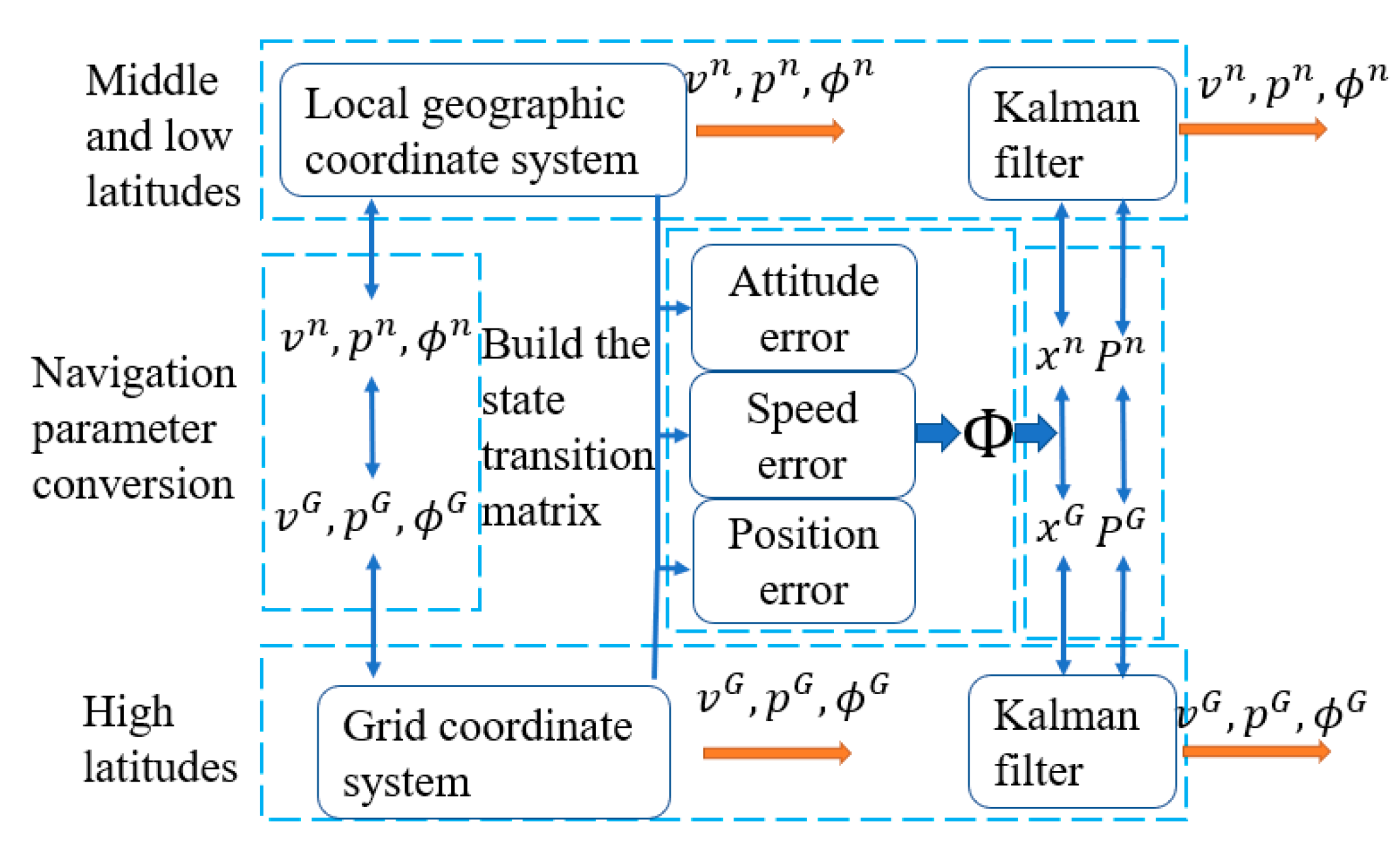
The process of the covariance transformation method is shown in
Figure 2. At middle and low latitudes, the system accomplishes the inertial navigation mechanization in the n-frame. When the aircraft enters the polar regions, the system accomplishes the inertial navigation mechanization in the G-frame. Correspondingly, the navigation parameters are output in the G-frame. During the navigation parameter conversion, the navigation results and Kalman filter parameter can be established according to the proposed method.
4. Experimental Results
This section presents the experiment and simulation results. A high-precision ring laser gyro inertial navigation system is used to conduct flight experiments. The ring laser gyro bias stability is less than 0.01°/h. The accelerometer bias stability is less than 20 μg. The GNSS positioning error is less than 10 m, which is used as the position reference. The update frequency of the gyro and accelerometer is 200 Hz, while the update frequency of GNSS is 1 Hz.
4.1. Flight Experiment
Flight experiments were carried out at middle latitudes. The duration was 4 h, including a half-hour’s alignment. Firstly, the experiment was carried out based on the n-frame. After flying for half an hour, the navigation frame was changed to the G-frame until the end of the flight.
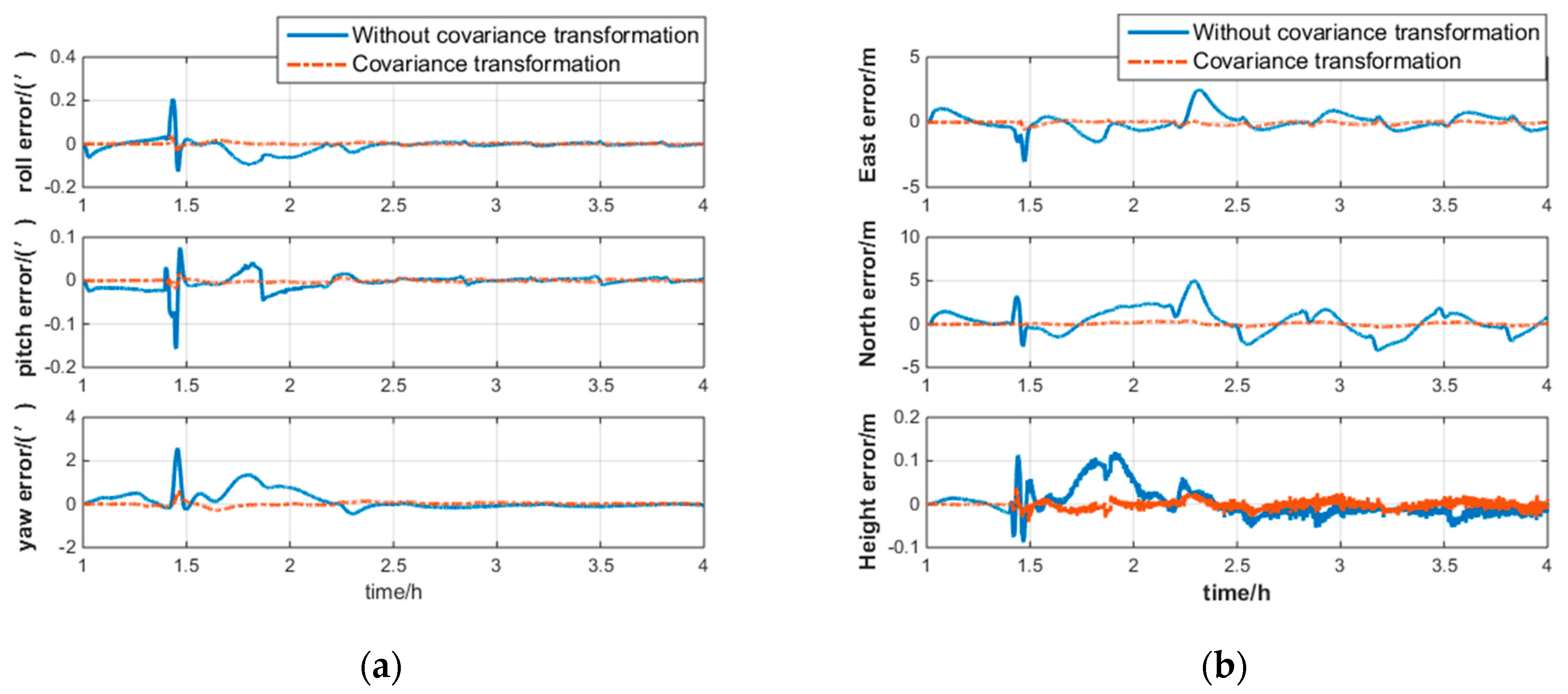
In order to evaluate the effects caused by navigation frame transformation, the results that are based on a local horizontal geographic frame are used as reference. Because the flight experiments are conducted at middle latitudes, there is no algorithm error introduced by the choice of navigation frame. The reference result is reliable. The navigation results, based on the covariance transformation and non-covariance transformation, are shown in
Figure 3.
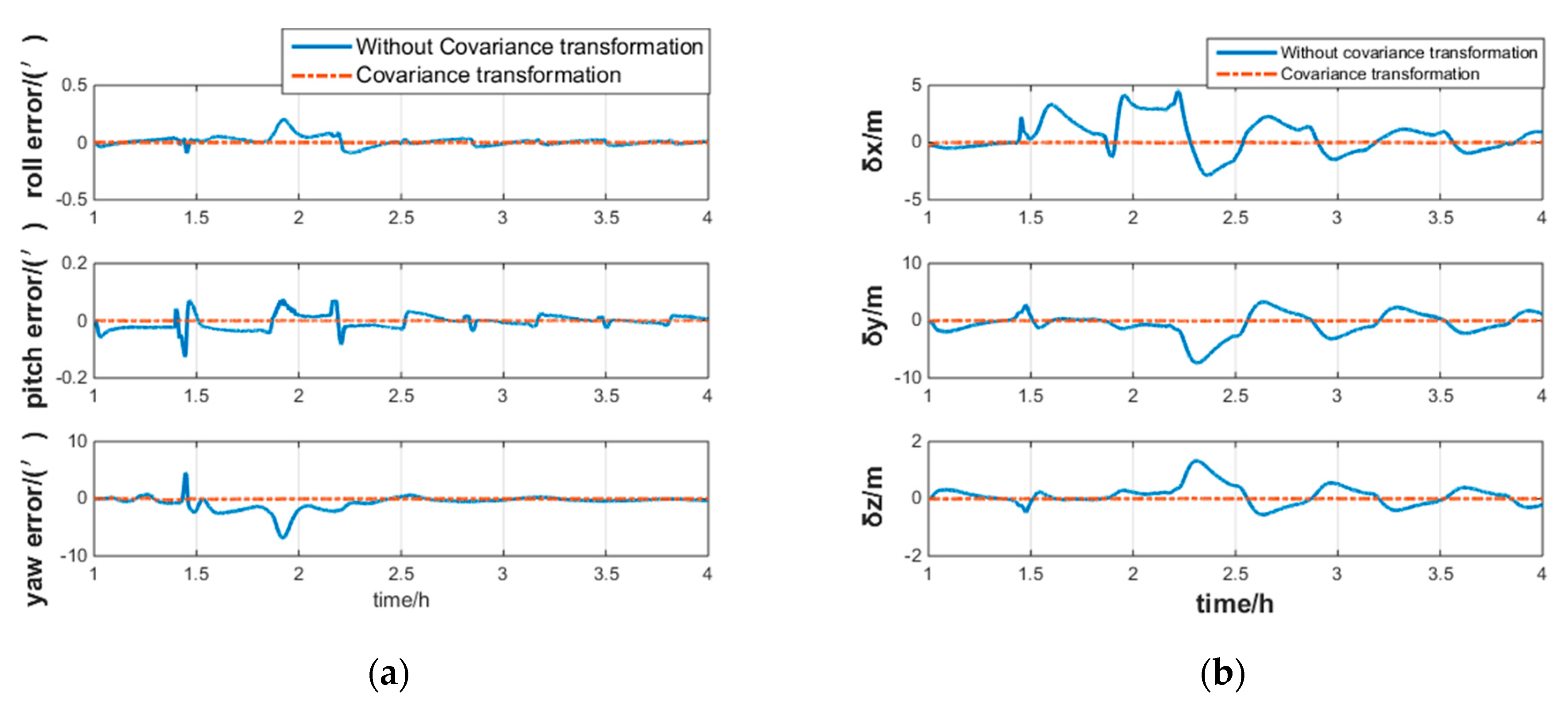
As shown in
Figure 3a, the change of the filter structure results in a fluctuation of the relative attitude error. Among the attitude errors, the relative yaw error reaches the maximum value of 2.2 ‘without covariance transformation. As a comparison, the covariance transformation method reduces this error to 0.3’.
Figure 3b shows that the relative position error is less than 10 m, regardless of whether the covariance transformation is used. The INS/GNSS-integrated navigation filter uses the position information provided by GNSS as observations to correct the INS results, resulting in less position error. As shown in
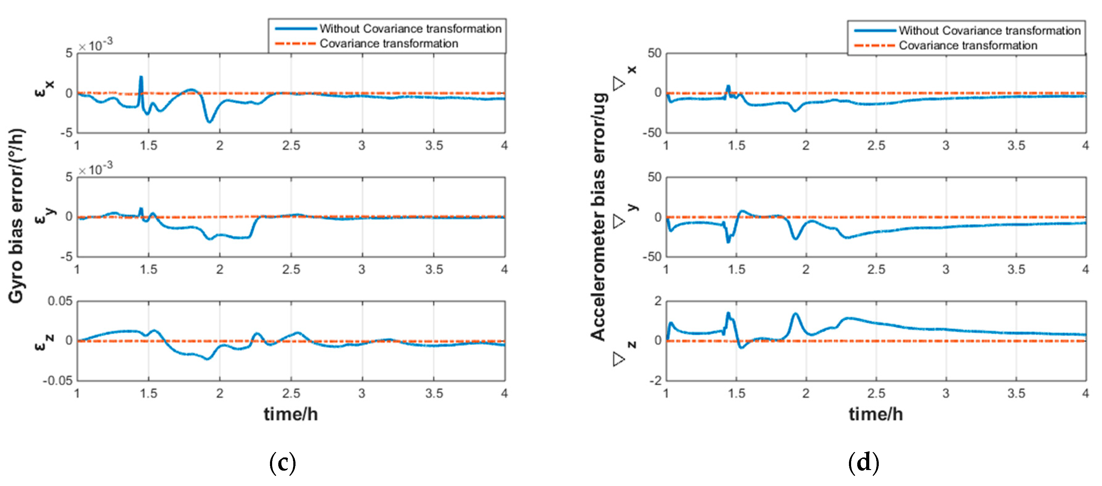
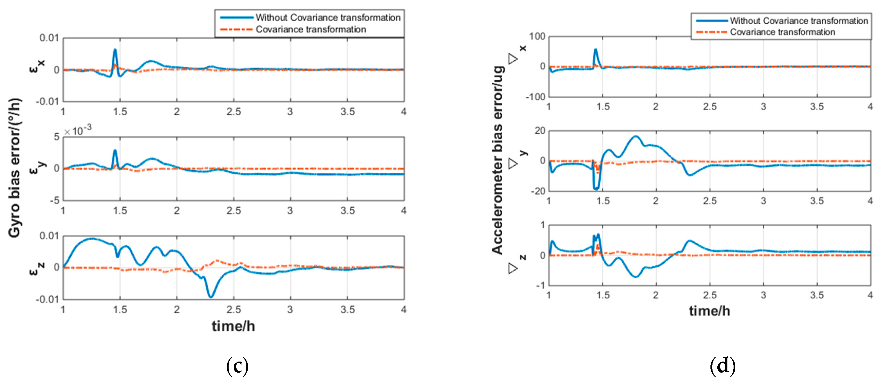
Figure 3c,d, the maximum bias error of the gyroscope with and without covariance transformation reaches 0.003°/h and 0.01°/h, respectively. The maximum bias error of the accelerometer with and without covariance transformation reaches 6 μg and 50 μg, respectively. Because of the non-zero values of the non-diagonal elements in the covariance matrix, the bias estimates of the gyroscope and accelerometer are affected by the cross-coupling of other error states. As a result, the bias estimates of the gyroscope and accelerometer also show instability.
The flight experiment was repeated six times. The results of the experiments are shown in
Table 1 and
Table 2.
To sum up, when the navigation frame changes directly, the integrated navigation results show severe fluctuation, taking more than an hour to reach stability again. The lower the observability of the error state, the larger the error amplitude. The integrated navigation results, based on the covariance transformation method, do not fluctuate during the change of the navigation frame, which is consistent with the reference results. Experimental results confirm the effectiveness of the proposed algorithm.
4.2. Semi-Physical Simulation Experiment
Pure mathematical simulation is difficult to use to accurately simulate an actual situation. Thus, a virtual polar-region method is used to convert the measured aviation data to 80° latitude, to obtain semi-physical simulation data [
20]. In this way, the reliability of the algorithm at high latitudes can be verified. In this simulation, the navigation result based on the G-frame is used as a reference, which will avoid the decrease of algorithm accuracy caused by the rise in latitude. The simulation results, based on the covariance transformation and non-covariance transformation, are shown in
Figure 4.
As can be seen in
Figure 4a, among the attitude errors, the relative yaw error is the largest. The relative yaw error reaches 5 ‘without covariance transformation. The integrated navigation result with covariance transformation has a less relative yaw error of 0.2’. As shown in
Figure 4b, the relative position error is 12 m, without covariance transformation. The integrated navigation result with covariance transformation shows better stability and a smaller relative position error of 8 m. As shown in
Figure 4c,d, the maximum bias error of the gyroscope with and without covariance transformation reached 0.001°/h and 0.02°/h, respectively. The maximum bias error of the accelerometer, with and without covariance transformation, reached 0.1 μg and 25 μg, respectively.


