Unsteady Flow Characteristics of an Oscillating Piezoelectric Fan Blade at High Reynolds Numbers

Abstract

Piezoelectric fans have started to play an essential role in small-scale heat removal applications in recent years due to their high reliability and efficiency. In this study, an experimental study on the flow field characteristics produced by an oscillating piezoelectric fan at various Reynolds numbers (140 < Re < 550) in a quiescent air environment is investigated. Time resolved particle image velocimetry (PIV) measurements are performed for the flow field visualization. The flow pattern generated by the oscillating fan blade in the longitudinal plane changes as the Reynolds number increases. The ratio between the trailing edge velocity and side edge velocity increases as the Reynolds number increases. As a result, the trailing edge plays a more important role in driving fluid at a higher Reynolds number. Multiple vortexes are shed from the trailing edge during one oscillation cycle and is observed only at a high Reynolds number. This vortex shedding increases the unsteadiness of velocity field significantly, resulting in a turbulence intensity level beyond 100%. This result implies that turbulence models used in numerical studies need to be carefully validated as some might struggle at this highly turbulent flow regime.

1. Introduction

Thermal management has become one of the important design considerations for electronics as devices keep reducing in size [1]. Due to the limited space, the natural convection is ineffective for heat dissipation, and this makes an extra cooling device crucial in this scenario [2]. Comparing to conventional rotatory fans in the field of electronic cooling, piezoelectric (PZT) fans have received more attention in recent years because of the advantages of low power consumption, high reliability and the small geometric deformation to generate a significant airflow [3,4]. A typical PZT fan consists of a blade and a PZT actuator. The PZT actuator is clamped to a stationary base at one end, whereas the fan blade is installed on the other free end. When an alternating high voltage is applied to the PZT actuator, the free end vibrates with the same frequency as the input signal. When the input signal frequency is tuned to the resonance frequency of the fan blade, the oscillating amplitude is significantly amplified, resulting in a useable airflow speed [5].

Previous studies have focused on the lift, thrust, mass flow and other characteristics that PZT fans can provide in relation to thermal and mechanical applications. Eastman et al. [6] tested the thrust of a piezoelectrically actuated oscillating cantilever in different Reynolds numbers and correlated it with the vibration amplitude. Stafford and Jeffers [7] discussed the bulk pressure-flow rate performance and efficiency characteristics of confined PZT fans. A recommended operating range was given between the points of maximum efficiency and maximum flow rate from the experiment results. Prince et al. [8] discussed the ionic polymer metal composite (IPMC) cantilever vibrating hydrodynamics in water.

More detailed studies on the characteristics of the flow field induced by PZT fans and the underlying mechanism have been performed both theoretically and experimentally. Kim et al. [9] investigated the velocity field of a vibrating cantilever plate using PIV. A Y-shape pseudo-jet flow dominated by vorticial structures was found beyond the plate tip. They obtained individual vortex information such as the size, strength, distribution and position by wavelet analysis for single phase data. Meanwhile, they applied the proper orthogonal decomposition (POD) technique to deduce the transient evolution process of the regional vortex. Hu et al. [10] conducted a phase-locking PIV experiment on a root-fixed piezoelectric flapping wing in a wind tunnel. Different vortex behaviors are found at different wingspans. The inner half close to the wing root produces drag, whereas the outer half was found to produce thrust. Besides, the flapping wing was also found to lift producing when it was mounted with a positive static angle of attack. Conway et al. [11] applied PIV technique and numerical method to study the effect of the thickness of a cantilever plate on the flow structure. They concluded that as the beam became thicker, the wake was dominated by the lateral jet region and the propagation of vortices was prevented. Moreover, they suggested vorticial structures were consistent with bluff body aerodynamic theory.

Multi-angle PIV measurements are also adopted to show the flow field details. Bidakhvidi et al. [12] investigated the flow field in both longitudinal and transverse planes of the fan blade using PIV measurement. Vortices and jet-like flow generated at the PZT fan tip were presented under different plane positions correlated with the Keulegan–Carpenter (KC) numbers. Eastman and Kimber [13] pointed out that the flow in the region near the corner of the oscillating cantilever beam would become extremely three-dimensional, i.e., two-dimensional measurements can hardly reflect the real flow structure around these regions. They made PIV measurements in both longitudinal and transverse planes at multiple locations to obverse the two-dimensional flow affected by the sharp edges.

The three-dimensional flow field induced by PZT fans is studied recently. Oh et al. [14] developed a three-dimensional simulation model for the confined vibrating flat plate. They claimed that the interaction of side vortices and tip vortices produced by confined piezoelectric fans lead to the velocity defect near the end wall, which agreed with the experimental data. Agarwal et al. [15] performed 3D phase-locked PIV measurements for the flow structure of an unconfined piezoelectric fan working at its first vibration mode. The structures of the vortex generated by the oscillation were constructed by interpolated PIV data, which initially appears as a horseshoe; the vortices generated by side edges form the two legs of the horseshoe vortex, then the tip-induced vortex separate from the trailing edge and formed into a hairpin shape with two legs still connect the blade tip. Numerical simulations were also performed to confirm the PIV result. Ebrahimi et al. [16] conducted 2D and 3D PIV measurements and numerical simulations to obtain detailed jet flow and vortex structures generated by the oscillation of a PZT fan with different oscillating frequency, amplitude and geometric parameter. They found that the breakdown of the shed vortex from the cantilever tip and the reorientation of the substructures are the primary factors that affect the shape of the induced jet.

From the literature mentioned above, effects of the thickness, frequency and amplitude of a PIZ fan blade on the flow field have been investigated in two-dimensional cases. Most 3D flow field measurements mainly focus on the evolution of the flow structures within one oscillating period for the same parameter. Few three-dimensional measurements have been conducted to investigate effects of fan blade geometry and oscillating frequency and amplitude. With the increase in the oscillating Reynolds number, the flow produced by the oscillating blade becomes more unsteady. In the current study, three-dimensional flow fields induced by a PZT fan blade in an unconfined quiescent air environment are measured at Reynolds numbers up to 550. The higher Reynolds number investigated in this study is more consistent with the piezoelectric fan operating condition in real applications.

The level of turbulence in the flow field induced by a piezoelectric fan is closely related to the performance of the piezoelectric fan. A high level of turbulence indicates a large kinetic energy loss, resulting in a less efficient fan to drive the fluid. However, a high level of turbulence can also increase the heat transfer coefficient. The overall role of turbulence generated by the piezoelectric fan blade on the heat dissipation is very complicated and still not clear. So far, there have been few studies focused on the turbulence characteristics generated by a piezoelectric fan blade. In the current study, the turbulence intensity levels at different Reynolds number conditions are evaluated, the maximum turbulence intensity at high Reynolds numbers up to 14.

The paper is organized as below. Section 2 introduces the PIV experiment setup and the measurement procedures. Section 3 presents the experiment results and discussion of the flow characteristics induced by the oscillating PZT fan blade. Section 4 concludes this study.

2. Experiment Methodology

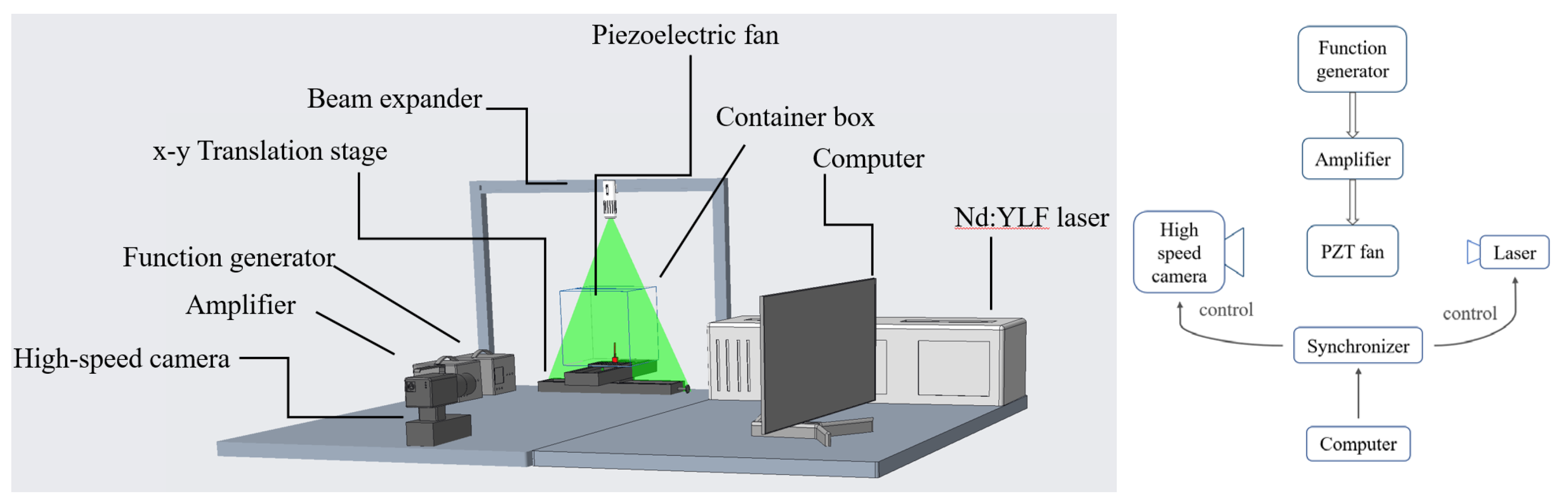
The experiment system for the flow field visualization is shown in Figure 1. The PZT fan (Sinocera Piezotronics, Yangzhou, China) is mounted at the bottom of a container box in the central position. The container box is made of transparent acrylic glass for observation and illumination. The space inside the container is large enough (300 mm × 300 mm × 300 mm) to avoid the sidewall effect. The container box is sealed so the outside environment can not interfere with the flow field inside this box. The container box is fixed on an x-y translation stage driven by two stepper motors (GCD-202002M, Daheng Optics, Beijing, China) with a resolution of 0.001 mm. The translation stage is used to adjust the position of the PZT fan blade relative to the laser sheet.

The performance of the PZT fan blade can be correlated to the vibrating frequency f and tip-to-tip amplitude A. In order to achieve the maximum amplitude, the vibrating frequency is fixed at the resonance frequency f_r = 58 Hz. The tip-to-tip vibration amplitude can be adjusted by changing the AC voltage applied to the PZT actuator. In this study, we select a series of different voltages to reach different vibration amplitudes in the range of 4.77 mm < A < 18.72 mm. The vibrating tip-to-tip amplitude A is measured optically by a pixel-analysis method, the tip position is determined by marking the pixels where the blade tip is at its maximum amplitude. The uncertainly of the pixel-analysis method is ±0.09 mm, corresponding to 1 pixel in the image. The characteristic tip velocity of the PZT fan is defined as:

$$U_{\mathrm{t}}=2fA$$

(1)

which is the average velocity of the trailing edge in a cycle. The geometrical parameters of the PZT fan blade include the length l_b, the width w_b and the thickness, t_b. The geometrical parameters of the PZT fan blade are fixed in this study with l_b = 65 mm, w_b = 15 mm and t_b = 0.1 mm (See Figure 2), resulting in an aspect ratio (AR = w_b/l_b) around 0.23. We adopted the definition of oscillatory Reynolds number Re [16] as:

$$Re=\frac{U_{\mathrm{t}}{w}_{\mathrm{b}}}{4v}=\frac{fA{w}_{\mathrm{b}}}{2v}$$

(2)

where ν = 14.8 × 10⁻⁶ m²/s is the kinematic viscosity of the air. The oscillatory Reynolds number in this study is in the range of 140 < Re < 550. The sinusoidal voltage for actuating the PZT fan blade is generated by a function generator (SDG 1062X, SIGLENT, Shenzhen, China) and an amplifier (ATA-2042, Aigtek, Xi’an, China).

A 527-nm double-pulse Nd:YLF laser (Vlite-Hi-527-40, Beam Tech, New Taipei, China) is used to illuminate the measurement region. The laser beam is expanded into a one-millimeter-thick laser sheet in the focused area. A high-speed camera (FASTCAM Nova S12 type 200KS-M-32G, Photron, Tokyo, Japan) is used to record the images. A laser pulse synchronizer (TSI Model 6130036 LASERPULSE) is used to control the pulsed laser and the high-speed camera. The interval time Δt between two laser pulses is set at 60 μs, i.e., the interval time between two PIV images in a pair is 60 μs. In this study, the maximum induced air velocity is less than 2 m/s, corresponding to 0.12 mm of particle displacement, so the time is short enough to enable the velocity calculation. The capture rate is set to 5800 Hz, which is 100 times of the oscillating PZT fan’s frequency f. In this way, 100 pairs of PIV images can be acquired within a single period of oscillation, equivalent to 5800 pairs of PIV images per second. The image resolution was set to 1024 × 1024 pixels with 12 bits per pixel. Seeding particles were generated by a Laskin nozzle oil droplet generator using olive oil. The air-oil droplet mixture is settled for 5 min before the PZT fan is actuated.

The image pre-processing and post-processing are performed using the commercial software TSI Insight 4G. A subtraction operation is performed by subtracting a minimum image to remove the background. The minimum image is generated by the minimum intensity method. Then, the multiplication operation is performed to every pixel in order to improve the image luminance; the operation does not eliminate image noise but makes the image clearer. The pre-processed images are then loaded to the PIV algorithm using a recursive Nyquist grid with an overlap gird spacing of 50%. The interrogation window size refines from 64 × 64 pixels to 32 × 32 pixels, ensuring at least 15 particles exist in the interrogation area. An FFT correlator is chosen as the correlation engine, and a Gaussian Peak with the signal to noise ratio of 1.5 is used for the peak engine. The calculated velocity is first validated globally by a standard deviation velocity range filter at a standard deviation factor of 7. It is subsequently validated locally using a median test method with a 5 × 5 pixels neighborhood size. The holes in the data were filled recursively using a local mean method with a 5 × 5 pixels neighborhood size. Finally, smoothing is performed after all the post-processing procedures, with a filter size of 5 × 5 pixels and sigma value of 0.8.

The 3D vortex structure was constructed by combining a group of 2D transverse plane along the y axis, 1 mm apart (see Figure 3). The transverse measurement plane was first placed at the midspan. After each PIV measurement, the plane translated along the positive direction of the y axis for d_shify,y = 1 mm. Due to the symmetric nature of the PZT fan blade, 16 planes are extracted from the midspan of the blade to the plane 15 mm away from the midspan in +y direction. To better visualize the 3D vortex structure, the measured data is mirrored at the mid-span to construct the other half. The 3D vortex structure at each phase is (defined in the next section) constructed by 32 2D ensemble-averaged flow field image. This procedure is also used in other studies [15,16,17].

3. Results

3.1. Time

In the current study, the time-averaged flow field is obtained from the PIV measurements in both longitudinal (y-z) and transverse (x-z) planes. In order to obtain the time-averaged flow field, 2000 pairs of PIV images were captured under the recording frequency, which is equivalent to 20 cycles of PZT fan oscillation. Figure 4 shows the contour of the time-averaged velocity magnitude (U_mag,yz) in y-z plane ranging from Re = 140 to 550, which is achieved by increasing the oscillation amplitude of the PZT fan. A slight asymmetricity about the midspan is observed, which might occur due to the material flaw of the fan blade and other disturbances in the testing environment. At a low Reynolds number (Re = 140), the amplitude of the PZT blade is relatively small. The flow field can be characterized into three main regions with large velocity magnitude. They are two regions near side edges and the region at the trailing edge of the PZT fan blade. As the Reynolds number increases (Re = 241 or 349), the time-averaged flow pattern changes. The high velocity regions expand and intensify, and the regions near the two side edges of the blade gradually converge with the high velocity region at the trailing edge. As the Reynolds number further increases, the three regions of high velocity observed in previous cases cannot be distinguished, and the airflow driven by the side edges and the trailing edge form a single high velocity region and propagate toward the streamwise direction along the midspan of the fan blade.

Based on the observation from Figure 4, the high velocity region is mainly generated at the side edges at the low Reynolds number and at trailing edge at the high Reynolds number. Here, the average flow velocity magnitude at the trailing edge is denoted as U_main and the average flow velocity magnitude at the two side edges of the blade is denoted as U_side, as shown in Figure 5. The velocity ratio can then be defined as R_U = U_main/U_side. As shown in Figure 4b, the velocity ratio R_U increases linearly with the Reynolds number. This means the averaged velocity at the trailing edge increases faster than the averaged velocity at the side edges as oscillation amplitude increases. When the R_U increases to a high level, the flow generated at the side edges is entrained by the flow at the trailing edge, forming a single high velocity region. An empirical correlation of R_U as a function of Re can be obtained as:

R_U = 0.0013 Re^1.1

(3)

Figure 6 shows the time-averaged velocity profile along the line of y = 0 and z = 0 on the longitudinal plane. Along the line y = 0 towards the +z direction (Figure 6b), at higher Reynolds number conditions (Re = 550 and 427), the magnitude of velocity decreases monotonically when moving away from the trailing edge. For the case of Re = 349, the velocity magnitude decreases rapidly in the first 10 mm. Then the slope became flat as the flow from the side of the blade joined the mainstream. Along the +y direction (Figure 6c), for higher Reynolds number cases (Re = 550 and 427), the velocity magnitude decreases monotonically and a turning point can be identified at approximately y = 12.5 mm. For the rest of the cases, the velocity decreases rapidly before the corner of the blade is reached and then the velocity increases again as the flow generated at the side edges of the blade comes to effect. From the experiment, the flow field in the longitudinal plane is affected jointly by the side edges and the trailing edge of the PZT fan blade.

Figure 7 shows the time-averaged velocity magnitude fields in the transverse plane for different Reynolds numbers. In general, the flow pattern in the transverse plane presents a “Y” shape, which is consistent with the findings of Kim et al. [9]. The high velocity region develops into two jetting shapes and these two jets are symmetrical about the z- axis. In the region between two jets, the velocity magnitude is comparatively lower. We selected two phases when the blade is in the middle position but moving towards different directions. These two phases are defined as phase τ = 0.25 and phase τ = 0.75 in the next section. The ensemble-averaged velocity magnitude fields at these two phases are obtained using 200 pairs of PIV images captured at the same position. Figure 8a,b is the U_x and U_z extracted from the midspan line, ranging from 0 < z < 40 mm. Figure 8c,d is the U_x and U_z extracted from the line parallel to the midspan line, with a distance of 15 mm away from the midspan, also ranging from 0 < z < 40 mm. The midspan line passes through the area between the two jets and the second line crosses one jet on the right-hand side. The velocity component in the x-direction of airflow generated at the tip area changes signs periodically as the blade oscillates. By performing time average, the x-component of velocity in this area is canceled out, resulting in the velocity magnitude in this area being lower compared to the jetting region, where the countering effect is comparatively weaker. In the transverse plane, the pattern of the flow field does not change considerably as the Reynolds number increases, but still the magnitude is alleviated, and the high velocity region is extended.

3.2. Vortex Evolution

The characteristics of the vortex generated by the vibration of the PZT fan blade is another key issue that has been widely discussed in previous studies. In order to obtain the vortex structure, an ensemble-averaged method for eight different phases τ was adopted here. Here, τ = t/T where t represents time and T is the time of an oscillation period. The position of the PZT fan blade at these phases are shown in Figure 9. For every single phase, 200 pairs of images are used for the ensemble averaging.

Figure 10 shows the ensemble-averaged result of x-component of vorticity (ω_x) generated in one cycle at Re = 550. The PZT fan blade tip moves from the rightmost position to the leftmost position in the first half period, then moves in the opposite way in the rest of the cycle. A clockwise (CW) vortex and a counterclockwise (CCW) vortex are generated in a single oscillation cycle. Starting from phase τ = 0, the blade starts to move, and a CW vortex starts to generate at the blade tip. The remnant of the CCW vortex from the previous cycle can be observed at this phase. As the blade accelerates and reaches the maximum velocity at phase τ = 0.25, the CW vortex is developed and the strength of the vortex core is intensified. Then the fan blade decelerates and starts to move in the opposite direction (phase τ = 0.375, τ = 0.5), resulting in the detachment and shedding of the CW vortex from the blade tip. Comparing the vortex generated under different Reynolds numbers, it can be found that the vortex develops in a similar procedure. As for the small Reynolds number case, the vortex basically dies out as the following vortex starts to generate and does not detach from the blade tip. As the Reynolds number increases, the vortex does not die out immediately when the movement of the blade changes direction. Instead, the vortex leaves the blade tip and propagates. In the case shown in Figure 10 with a relatively large Reynolds number (Re = 550), the vortex splits at the point when the movement of the tip starts to change direction (τ = 0, τ = 0.5), then the remnant vortex propagates to the downstream with the flow.

During an oscillation cycle, the intensity of the CW and CCW vortex changes. Figure 11 shows the variation of the maximum y-component CW and CCW vorticity during a cycle. For different cases, the tendency of the maximum ω_y is basically the same. The CW vortex reaches the maximum intensity around phase τ = 0.25 and the CCW vortex reaches the maximum intensity around phase τ = 0.75 for all cases. With the increase in the Reynolds number, the maximum intensity for both the CW and CCW vortexes are enhanced at different phases.

In order to visualize the evolution of the vorticity, the 3D vortex structure generated by the vibrating blade is illustrated. We adopted a similar strategy used in previous studies [15,16,17] to construct the vortex structure. The concept is described in detail in Section 2 of this paper. The 2D PIV transverse slice at different positions is combined. In Figure 12, the iso-surface of y-component of vorticity is used to visualize the vortex structure generated during a full cycle of the fan blade vibration at Re = 550. Because of the similarity of the CW and CCW vortex generated in a full vibration cycle, here we focus on the temporary evolution of the CW vortex structure. At the beginning of this cycle, as the PZT fan blade starts to move from the rightmost position to the left, a CW vortex, as previously observed in the transverse plane, starts to evolve. At this phase, the CCW vortex generated in the previous cycle starts to detach from the blade tip and the CW vortex generated in the previous cycle is dissipating.

At two side edges of the blade, there is also a vortex generated. Together with the vortex at the trailing edge, a horseshoe structure is formed, which has been shown in Figure 13a. The CW vortex continues to develop in the later phases and the head of the horseshoe vortex is elongated in x-direction. At phase τ = 0.5, when the blade changes the direction of movement, two distinct vortex rolls are observed. This demonstrates the shedding of the CW vortex. The vortex shed from the blade tip then develops into a hairpin structure (see Figure 13b) and gradually diffuses in the flow field. The part still connected to the blade tip eventually detaches as the blade moves towards the right, then it propagates and dissipates as traveling in streamwise direction. The formation of the horseshoe vortex and hairpin vortex is consistent with previous studies reported in [15,16].

Figure 14 illustrates the vortex structure generated by the PZT fan blade at different Reynolds numbers. At Reynolds number Re = 349, the generation, spreading, splitting, propagation and diffusion processes are basically the same when comparing to the case of Re = 550. The vortex shedding can also be observed. However, due to the lower vorticity strength, the iso-surface structure reduces in scale. As the Reynolds number further decreases to Re = 140, the two legs of the horseshoe vortex generated at the side edges are no longer observed due to the lower vortex core strength. Besides, the vortex at the trailing edge dies out soon after it was generated. No vortex shedding was observed at this Reynolds number.

3.3. Turbulence Characteristics

The results of instantaneous PIV measurement in previous research [16,18] and the ensemble-averaged result in Section 3.2 suggested that a strong turbulence effect exists in the flow field produced by the vibrating PZT fan blade. However, the turbulence characteristics of the flow field are seldom discussed in previous studies. To quantify the turbulence effect, we calculated the turbulence intensity using the PIV data, and the TI_xz is defined as:

$${TI}_{xz}=\frac{\overline{u_x^{\prime }{}^2}+\overline{u_z^{\prime }{}^2}}{{\overline{u_x}}^2+{\overline{u_z}}^2}$$

(4)

where $u_x^{\prime }$ and $u_z^{\prime }$ are the fluctuating parts of the x and z-component of the velocity in the transverse plane respectively; $\overline{u_x}$ and $\overline{u_z}$ are the x and z-component of ensemble-averaged velocity at this phase. Similarly, for the longitudinal plane, TI_yz can be calculated as:

$${TI}_{yz}=\frac{\overline{u_y^{\prime }{}^2}+\overline{u_z^{\prime }{}^2}}{{\overline{u_y}}^2+{\overline{u_z}}^2}$$

(5)

Figure 15a–c shows the result of turbulence intensity at different phases in the longitudinal plane for different Reynolds numbers. In order to better visualize the turbulence intensity pattern at a lower Reynolds number, we apply different color scales for different cases. For the lowest Reynolds number Re = 140, the maximum TI_xy is lower than 0.1 for all phases, indicating that the effect of turbulence on the flow field at a low Reynolds number is insignificant and negligible. For the case of Re = 347, the turbulence intensity is enhanced around the area of the blade trailing edge and two side edges. The turbulence intensity around these areas for this case is in the range of 0.1 < TI_yz < 0.5. When the Reynolds number increases to Re = 550, the turbulence is greatly enhanced at the trailing edge along the streamwise direction. In the area where the unsteady vortex is generated and shed, the turbulence intensity is increased to TI_yz = 1 and even above. Figure 15d quantifies the maximum turbulence intensity for each phase at different Reynolds numbers. At Re = 140, the maximum turbulence intensity corresponding to each phase is relatively low. When the Reynolds number reaches 550, the large oscillation amplitude greatly disturbed the flow field. The turbulence intensity is relatively small at τ = 0 and τ = 0.5, where the blade tip velocity is zero. It gradually increases with the growth of the vortices generated by the blade oscillation.

To evaluate the area affected by the turbulence, we calculated the area encompassed by the contour line of TI_yz = 0.05 at different phases as A_tur,yz. As can be seen in Figure 16, A_tur,yz is close to 0 at a low Reynolds number (Re = 140). As the Reynolds number increases to Re = 349, the A_tur,y is alleviated, ranging from 80 mm² to 170 mm². At Re = 550, the A_tur,y is further increased by almost 2 to 3 times.

Figure 17a illustrates the maximum turbulence intensity TI_xz,max at different phases in the transverse plane. Similar to the longitudinal plane, the maximum turbulence intensity is close to 0 for all phases when Re = 140. When the Reynolds number increases to 349, the TI_xz,max fluctuates between the 1 to 2, and the range is wider comparing to the longitudinal plane. At Re = 550, the TI_xz,max varies from 6 to 14. From Figure 17b, the area affected by turbulence at different phases extended as the Reynolds number increases. Comparing to the longitudinal plane, the A_tur,xz is larger at the same Reynolds number, which is due to the stronger vorticity exhibited in the transverse plane.

From the discussion above, it can be concluded that when the PZT fan is operating at a low Reynolds number, the turbulence effect can be ignored, but as the Reynolds number increases, the turbulence intensity level increases significantly, especially for the high Reynolds number conditions. This result suggests that turbulence model needs to be carefully validated in numerical studies when calculating high Reynolds number flows, as the turbulence intensity could be up to 100% and above. It is also important for optimizing cooling performance. As cooling efficiency increases as turbulence intensity level increases, the hot surface/source should be placed in the area where the intensity of turbulence is strong in order to improve cooling performance.

4. Conclusions

In the current study, the unsteady flow field characteristics induced by an oscillating PZT fan blade in a quiescent air environment was investigated. Time resolving PIV measurements were performed to visualize the flow structure in 2D and 3D. The flow field generated by the oscillating PZT fan blade was examined as the fan blade operates in the range of 140 < Re < 550. The flow pattern generated by the oscillating fan blade in the longitudinal plane changes as Reynolds number increases. It was found that the ratio between the trailing edge velocity and side edge velocity increases as the Reynolds number increases. Ratio of the trailing edge velocity and side edge velocity are approximately equal to 0.0013 Re^1.1. As a result, side edges contribute to the generation of high velocity at lower Reynolds numbers, whereas their contribution reduces at high Reynolds numbers. From the unsteady flow field analysis, the vortex shedding from the blade trailing edge was observed at high Reynolds number but not at low Reynolds number. This vortex shedding increases the unsteadiness of velocity field significantly at the high Reynolds number, where high turbulence intensity level beyond 100% was observed. The influencing area of turbulence also increases significantly at the high Reynolds number as the transient flow field due to large blade deflection vibrations is highly unsteady. This suggests that numerical studies for a PZT fan need to be carefully validated as some turbulence models can struggle at this highly turbulent flow regime.

References

1. Açikalin, T.; Wait, S.M.; Garimella, S.V.; Raman, A. Experimental Investigation of the Thermal Performance of Piezoelectric Fans. Heat Transf. Eng. 2004, 25, 4–14. [Google Scholar] [CrossRef] [Green Version]
2. Garimella, S.V. Advances in mesoscale thermal management technologies for microelectronics. Microelectron. J. 2006, 37, 1165–1185. [Google Scholar] [CrossRef] [Green Version]
3. Maaspuro, M. Piezoelectric oscillating cantilever fan for thermal management of electronics and LEDs—A review. Microelectron. Reliab. 2016, 63, 342–353. [Google Scholar] [CrossRef]
4. Hales, A.; Jiang, X. A review of piezoelectric fans for low energy cooling of power electronics. Appl. Energy 2018, 215, 321–337. [Google Scholar] [CrossRef]
5. Yoo, J.H.; Hong, J.I.; Cao, W. Piezoelectric ceramic bimorph coupled to thin metal plate as cooling fan for electronic devices. Sens. Actuators A Phys. 2000, 79, 8–12. [Google Scholar] [CrossRef]
6. Eastman, A.; Kiefer, J.; Kimber, M. Thrust measurements and flow field analysis of a piezoelectrically actuated oscillating cantilever. Exp. Fluids 2012, 53, 1533–1543. [Google Scholar] [CrossRef]
7. Stafford, J.; Jeffers, N. Aerodynamic Performance of a Vibrating Piezoelectric Blade Under Varied Operational and Confinement States. IEEE Trans. Compon. Packag. Manuf. Technol. 2017, 7, 751–761. [Google Scholar] [CrossRef]
8. Prince, C.; Lin, W.; Lin, J.; Peterson, S.D.; Porfiri, M. Temporally-resolved hydrodynamics in the vicinity of a vibrating ionic polymer metal composite. J. Appl. Phys. 2010, 107, 094908. [Google Scholar] [CrossRef]
9. Kim, Y.-H.; Cierpka, C.; Wereley, S.T. Flow field around a vibrating cantilever: Coherent structure eduction by continuous wavelet transform and proper orthogonal decomposition. J. Fluid Mech. 2011, 669, 584–606. [Google Scholar] [CrossRef]
10. Hu, H.; Clemons, L.; Igarashi, H. An experimental study of the unsteady vortex structures in the wake of a root-fixed flapping wing. Exp. Fluids 2011, 51, 347–359. [Google Scholar] [CrossRef]
11. Conway, C.; Jeffers, N.; Agarwal, A.; Punch, J. Influence of thickness on the flow field generated by an oscillating cantilever beam. Exp. Fluids 2020, 61, 1–19. [Google Scholar] [CrossRef]
12. Bidakhvidi, M.A.; Shirzadeh, R.; Steenackers, G.; Vanlanduit, S. Experimental study of the flow field induced by a resonating piezoelectric flapping wing. Exp. Fluids 2013, 54, 1–16. [Google Scholar] [CrossRef]
13. Eastman, A.; Kimber, M.L. Analysis of three-dimensional attributes and flow intake for an oscillating cantilever. Exp. Fluids 2014, 55, 1–14. [Google Scholar] [CrossRef]
14. Oh, M.H.; Park, S.H.; Kim, Y.-H.; Choi, M. 3D flow structure around a piezoelectrically oscillating flat plate. Eur. J. Mech.—B/Fluids 2018, 67, 249–258. [Google Scholar] [CrossRef]
15. Agarwal, A.; Nolan, K.P.; Stafford, J.; Jeffers, N. Visualization of three-dimensional structures shed by an oscillating beam. J. Fluids Struct. 2017, 70, 450–463. [Google Scholar] [CrossRef]
16. Ebrahimi, N.D.; Eldredge, J.D.; Ju, Y.S. Three-dimensional characteristics of the jet flows induced by a pitching plate in a quiescent fluid. J. Fluid Mech. 2020, 887, A25. [Google Scholar] [CrossRef]
17. Green, M.A.; Rowley, C.W.; Smits, A.J. The unsteady three-dimensional wake produced by a trapezoidal pitching panel. J. Fluid Mech. 2011, 685, 117–145. [Google Scholar] [CrossRef] [Green Version]
18. Ebrahimi, N.D.; Eldredge, J.D.; Ju, Y.S. Wake vortex regimes of a pitching cantilever plate in quiescent air and their correlation with mean flow generation. J. Fluids Struct. 2018, 84, 408–420. [Google Scholar] [CrossRef] [Green Version]
Figure 1. Schematic of PIV experiment setup.
Applsci 11 09510 g001
Figure 2. Geometry parameters of the PZT fan blade and the illuminated plane for the PIV measurement, with frame (a) showing geometry parameters (b) showing the transverse plane (x-z plane) and frame (c) showing the longitudinal plane (y-z plane).
Applsci 11 09510 g002
Figure 3. PIV measurement slices along the y axis with 1 mm apart in the transverse plane (x-z plane).
Applsci 11 09510 g003
Figure 4. Time-averaged velocity magnitude (Umag,yz) field of the y-z plane at different Reynolds numbers.
Applsci 11 09510 g004
Figure 5. Relation between RU (Umain/Uside) and Re: (a) definition of Umain and Uside, (b) variation of RU against Re.
Applsci 11 09510 g005
Figure 6. Velocity magnitude at streamwise and spanwise lines: (a) schematic of the lines for data extraction, (b) velocity magnitude profile of the flow field along the line of y = 0, 0 < z < 40. (c) Velocity magnitude profile of the flow field along the line of z = 0, 0 < y < 40.
Applsci 11 09510 g006
Figure 7. Time-averaged velocity magnitude (Umag,xz) field in the transverse plane (x-z plane) at different Reynolds numbers.
Applsci 11 09510 g007
Figure 8. Time averaged velocity profiles extracted at different streamwise lines: (a) Ux profile along the midspan line (x = 0, 0 < z < 40 mm), (b) Uz profile along the midspan line (x = 0, 0 < z < 40 mm), (c) Ux profile along the line distancing 15 mm away from the midspan line (x = 15, 0 < z < 40 mm) and (d) Uz profile along the line distancing 15 mm away from the midspan line (x = 15, 0 < z < 40 mm).
Applsci 11 09510 g008
Figure 9. Position of PZT fan blade for eight phases in an oscillation period.
Applsci 11 09510 g009
Figure 10. Evolution of y-component of vorticity (ωy) in one cycle at Reynolds number Re = 550.
Applsci 11 09510 g010
Figure 11. Maximum y-component of CW and CCW vorticity (ωy,max) at different phases.
Applsci 11 09510 g011
Figure 12. Temporal evolution of vortex in an oscillation period in 3D (Re = 550).
Applsci 11 09510 g012
Figure 13. Typical flow structures generated by PZT fan: (a) a CW horseshoe vortex at τ = 0.25, (b) a hairpin vortex at τ = 0.375.
Applsci 11 09510 g013
Figure 14. Temporal evolution of vortex in an oscillation period in 3D at different Reynolds numbers.
Applsci 11 09510 g014
Figure 15. Turbulence intensity TIyz in the longitudinal plane for different Reynolds numbers (Re = 140, 349, 550 for frame (ac), respectively) and (d) maximum turbulence intensity TIyz,max during one cycle at three Reynolds numbers.
Applsci 11 09510 g015
Figure 16. Influencing area of turbulence Atur,yz in different phases during one cycle at different Reynolds numbers.
Applsci 11 09510 g016
Figure 17. Turbulence characteristics during one cycle at different Reynolds numbers: (a) maximum turbulence intensity TIxz,max and (b) influencing area of turbulence Atur,xz at different phases.
Applsci 11 09510 g017
Publisher’s Note: MDPI stays neutral with regard to jurisdictional claims in published maps and institutional affiliations.