
An Integrated Spatio-Temporal Features Analysis Approach for Ocean Turbulence Using an Autonomous Vertical Profiler


Abstract
:1. Introduction
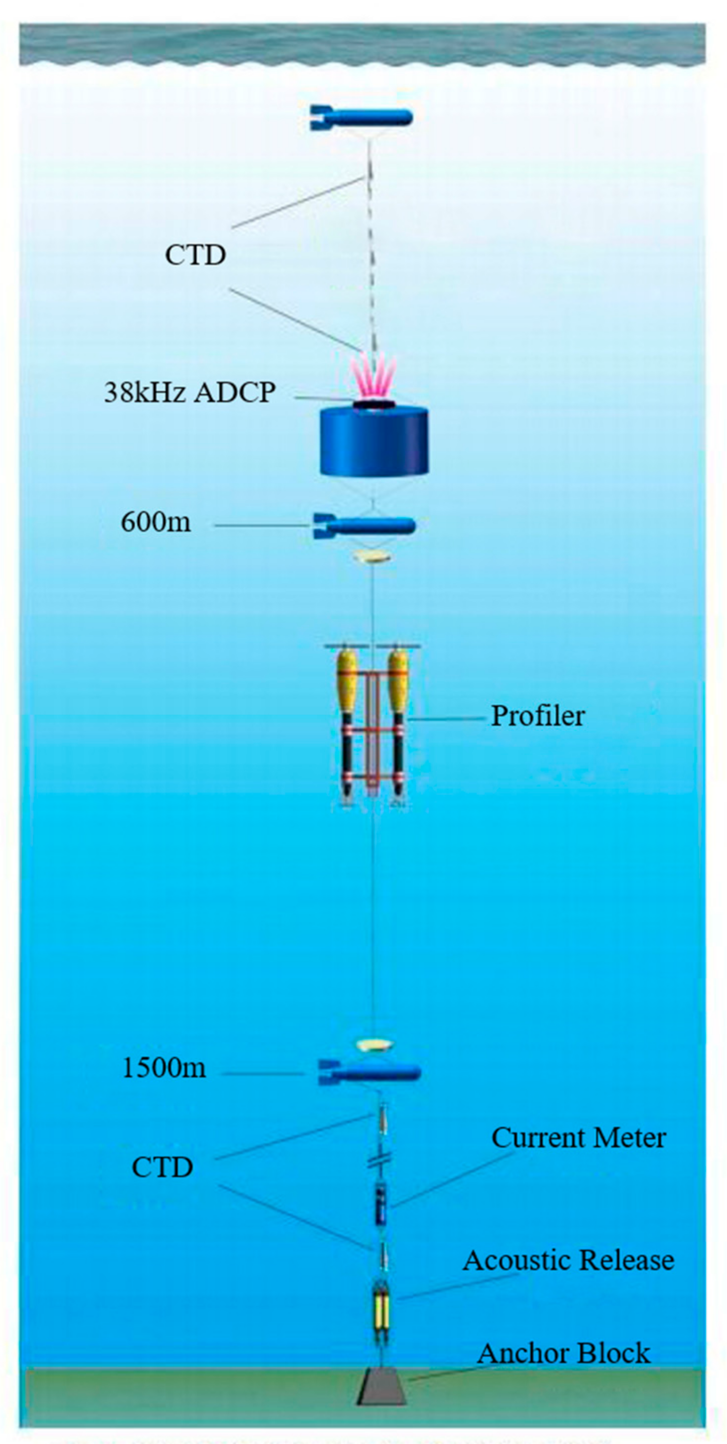
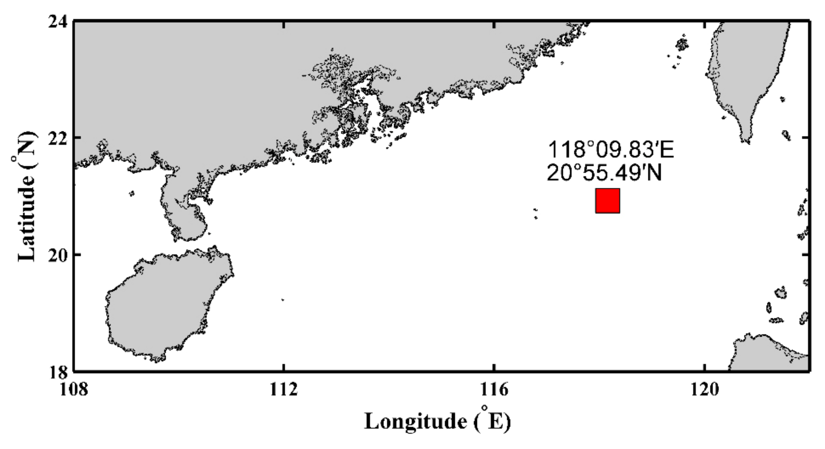
2. Experiments
3. Methodologies
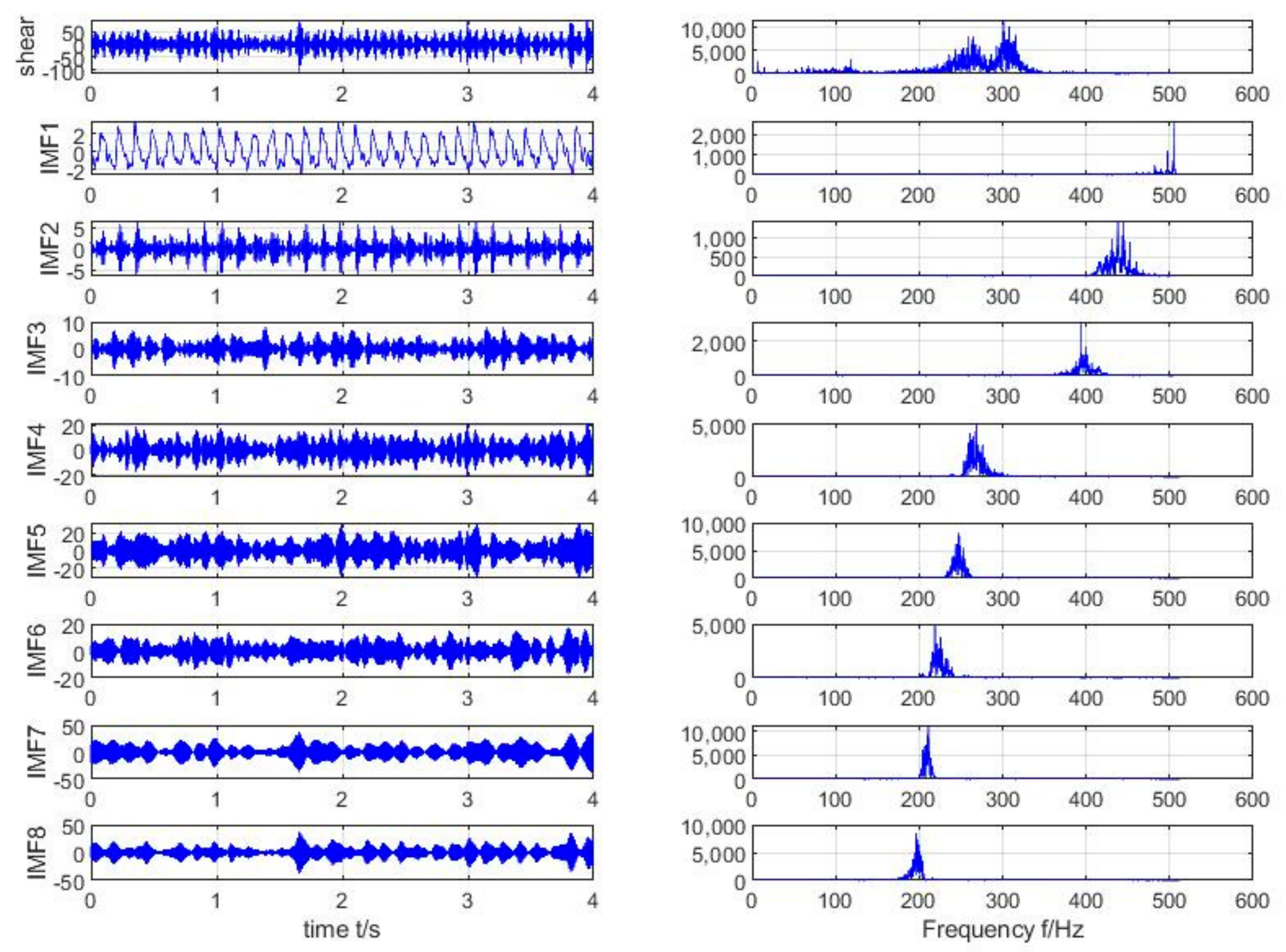
3.1. The VMD Decomposition
3.2. Wavelet Transforms
3.3. Local Measure of Intermittency
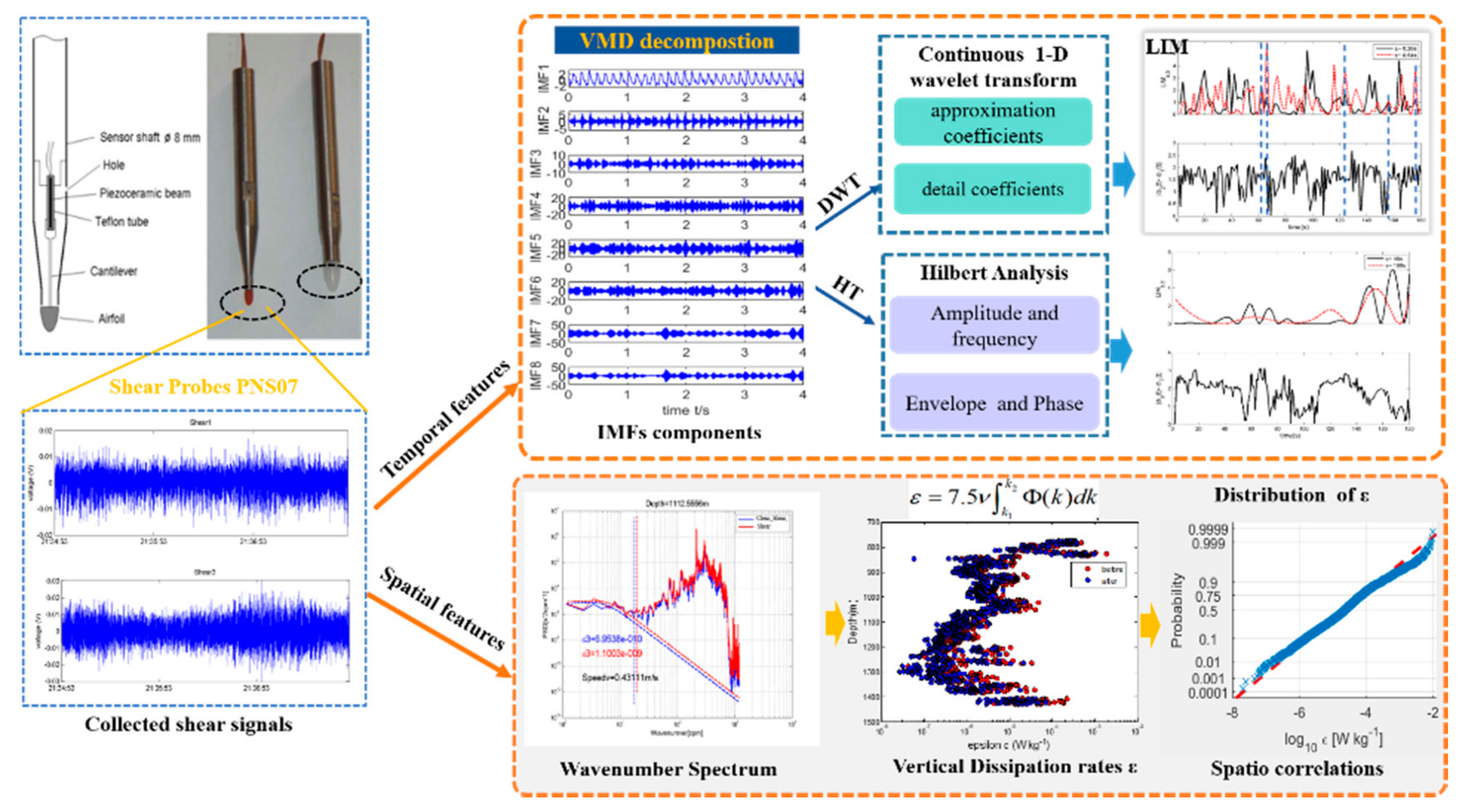
3.4. An Integrated Analysis Method
- Temporal features localization and quantitation.
- Spatial features identification.
4. Results
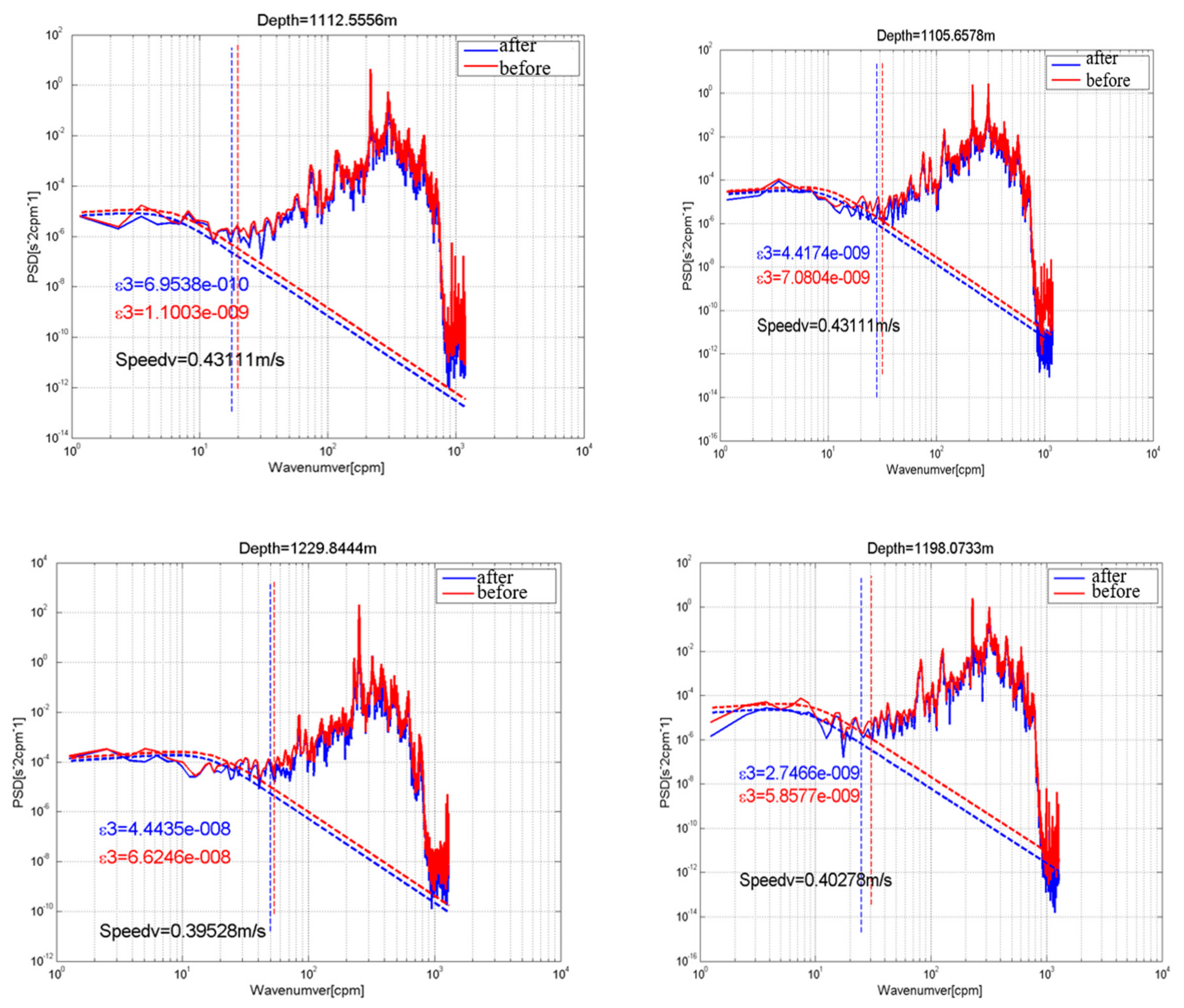
4.1. Features of Time-Frequency and Wavenumber Spectrum
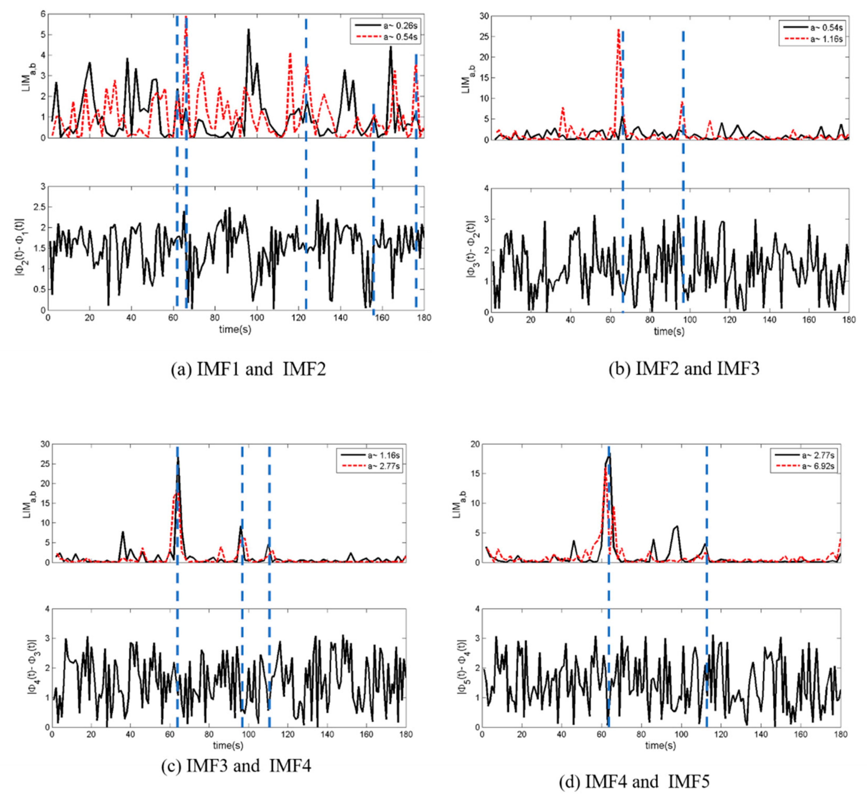
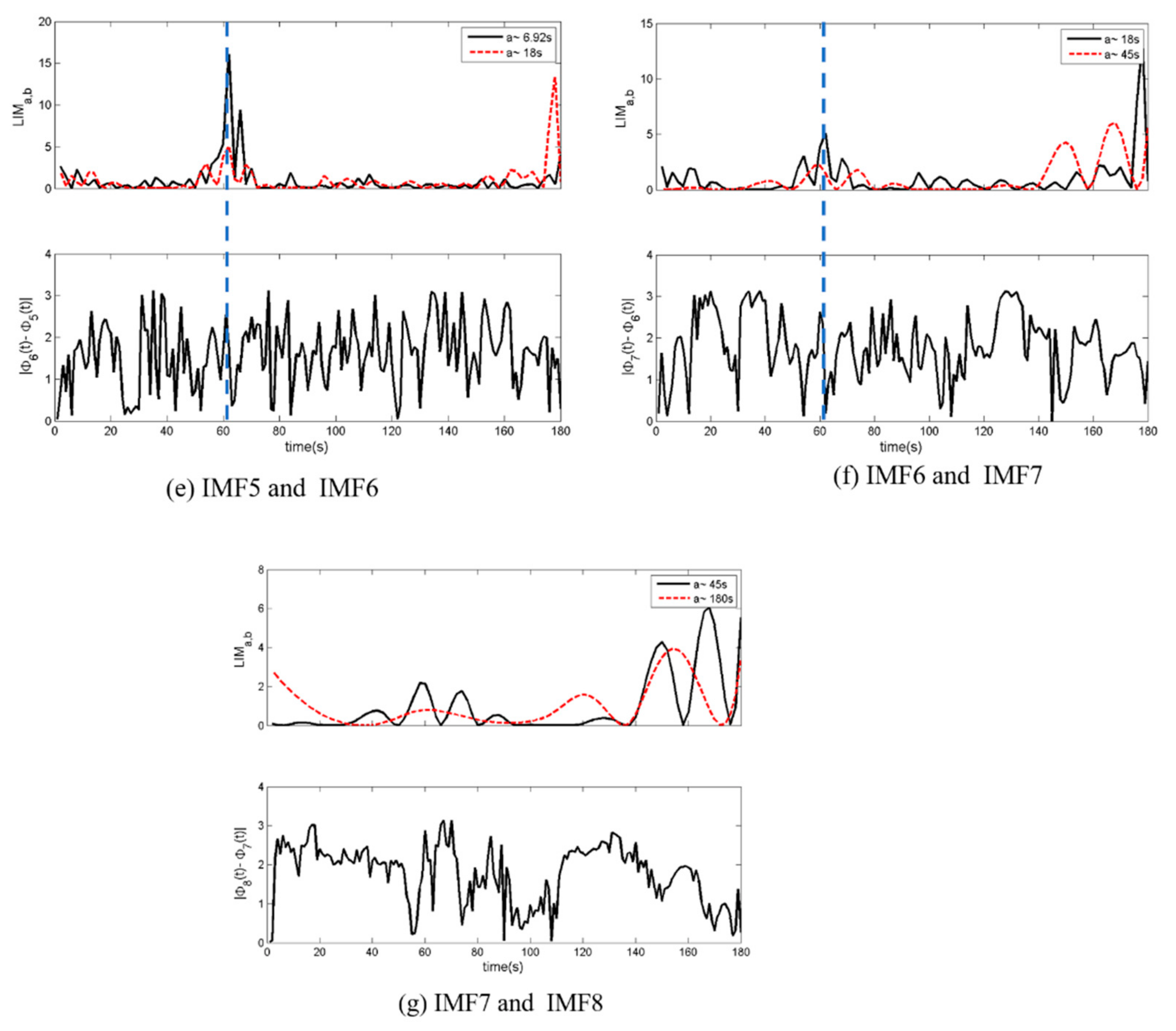
4.2. Temporal Features of Local Energy Cascade and Intermittency
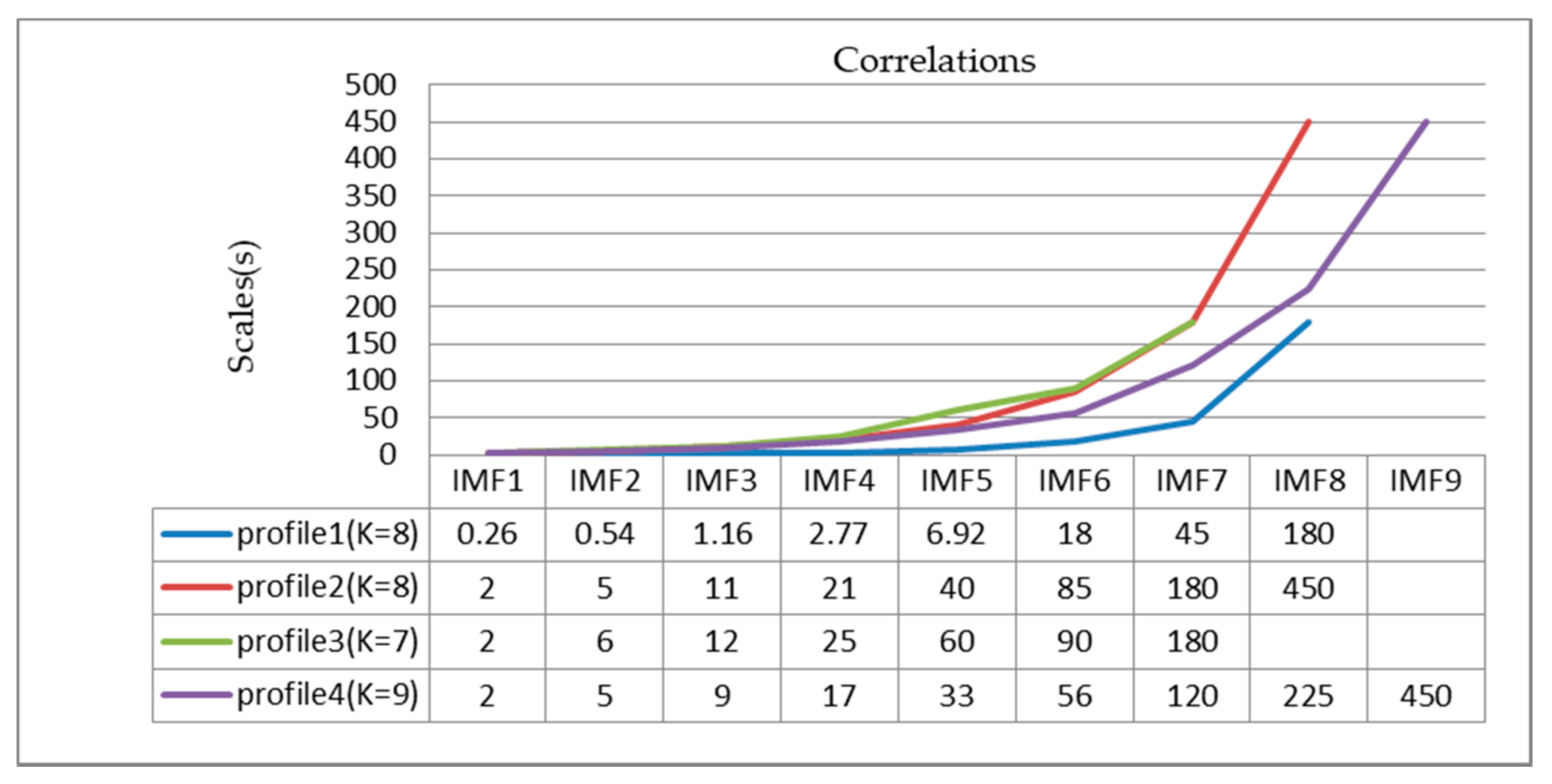
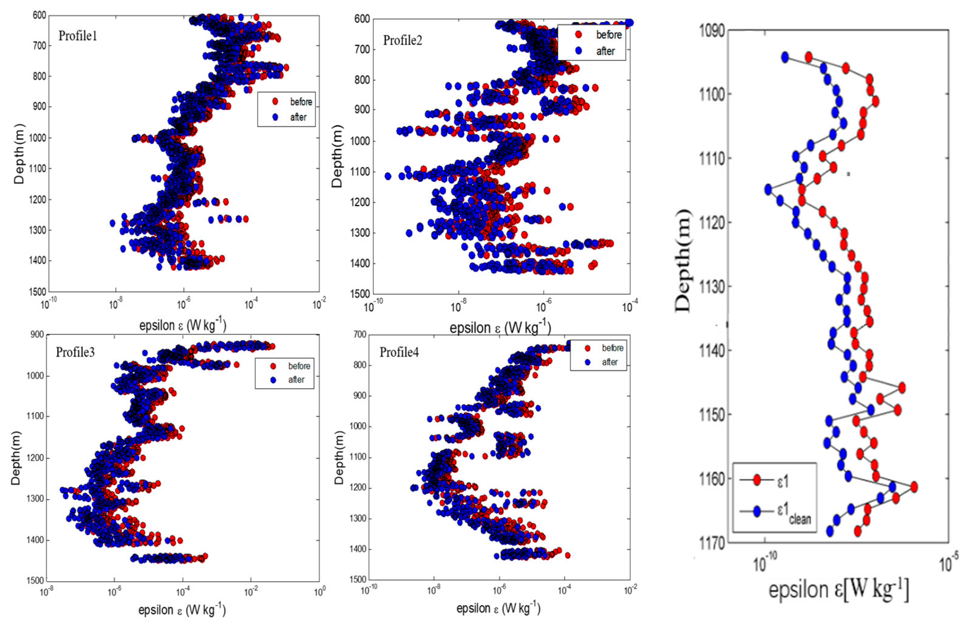
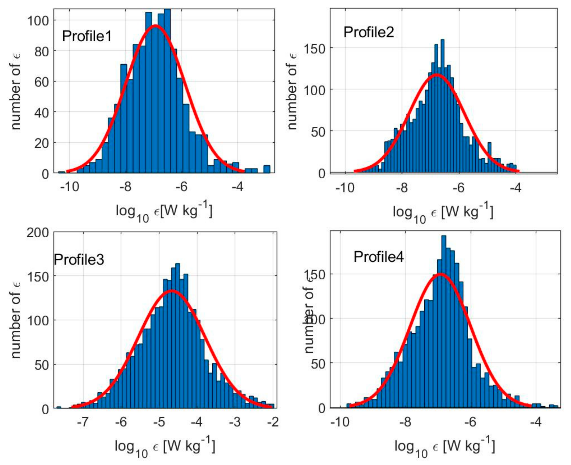
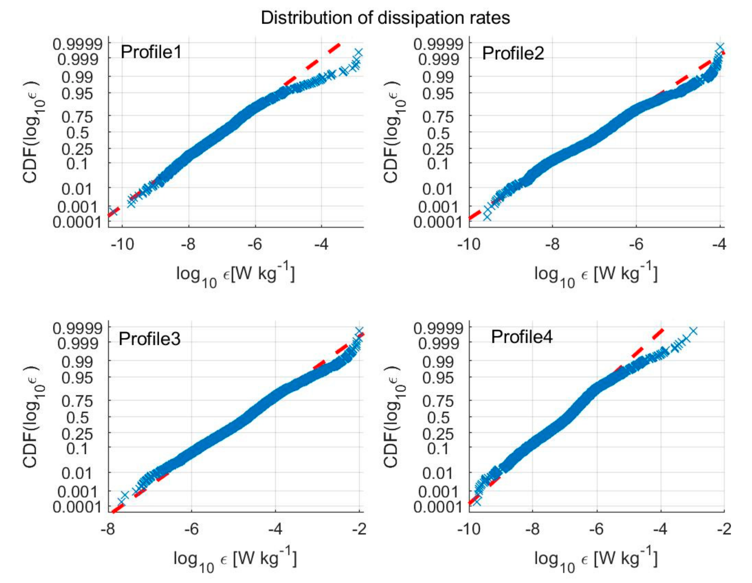
4.3. Spatial Statistical Characteristics of Dissipation Rates
5. Conclusions
Author Contributions
Funding
Institutional Review Board Statement
Informed Consent Statement
Data Availability Statement
Acknowledgments
Conflicts of Interest
References
- Qiu, B.; Chen, S.; Klein, P.; Sasaki, H.; Sasai, Y. Seasonal mesoscale and submesoscale eddy variability along the North pacific. subtropical countercurrent. J. Phys. Oceanogr. 2014, 44, 3079–3098. [Google Scholar] [CrossRef] [Green Version]
- Mckeown, R.; Ostilla-Monico, R.; Pumir, A.; Brenner, M.P.; Rubinstein, S.M. Turbulence generation through an iterative cascade of the elliptical instability. Physics. Flu. Dyn. 2019, 21, eaaz2717. [Google Scholar] [CrossRef] [Green Version]
- Eden, C.; Czeschel, L.; Olbers, D. Toward energetically consistent ocean models. J. Phys. Oceanogr. 2014, 44, 3160–3184. [Google Scholar] [CrossRef] [Green Version]
- Abernathey, R.; Wortham, C. Phase speed cross spectra of eddy heat fluxes in the eastern pacific. J. Phys. Oceanogr. 2015, 45, 1285–1301. [Google Scholar] [CrossRef] [Green Version]
- Onorato, M.; Camussi, R.; Iuso, G. Small scale intermittency and bursting in a turbulent channel flow. Phys. Rev. E 2000, 61, 1447–1454. [Google Scholar] [CrossRef]
- Perri, S.; Carbone, V.; Vecchio, A.; Bruno, R.; Korth, H.; Zurbuchen, T.H.; Sorriso-Valvo, L. Phase-synchronization, energy cascade, and intermittency in solar-wind turbulence. Phys. Rev. Lett. 2012, 109, 846–851. [Google Scholar] [CrossRef] [Green Version]
- Xu, C.; Li, L.; Cui, G.; Zhang, Z. Multi-scale analysis of near-wall turbulence intermittency. J. Turbul. 2006, 7, 1–15. [Google Scholar] [CrossRef]
- Foucher, F.; Ravier, P. Determination of turbulence properties by using empirical mode decomposition on periodic and random perturbed flows. Exp. Fluids 2010, 49, 379–390. [Google Scholar] [CrossRef]
- Arbic, B.K.; Scott, R.B.; Flierl, G.R.; Morten, A.J.; Shriver, J.F. Nonlinear cascades of surface oceanic geostrophic kinetic energy in the frequency domain. J. Phys. Oceanogr. 2012, 42, 1577–1600. [Google Scholar] [CrossRef] [Green Version]
- Arbic, B.K.; Polzin, K.L.; Scott, R.B.; Richman, J.G.; Shriver, J.F. On eddy viscosity, energy cascades, and the horizontal resolution of gridded satellite altimeter products. J. Phys. Oceanogr. 2013, 43, 283–300. [Google Scholar] [CrossRef] [Green Version]
- Zhdankin, V.; Uzdensky, D.A.; Boldyrev, S. Temporal intermittency of energy dissipation in magnetohydrodynamic turbulence. Phys. Rev. Lett. 2015, 114, 065002. [Google Scholar] [CrossRef] [Green Version]
- Camporeale, E.; Sorriso-Valvo, L.; Califano, F.; Retino, A. Coherent structures and spectral energy transfer in turbulent plasma: A space-filter approach. Physical Phys. Rev. Lett. 2018, 120, 125101. [Google Scholar] [CrossRef] [Green Version]
- Wang, W.; Pan, C.; Wang, J. Multi-component variational mode decomposition and its application on wall-bounded turbulence. Exp. Fluids 2019, 60, 1–18. [Google Scholar] [CrossRef]
- Vásconez, C.L.; Perrone, D.; Marino, R.; Laveder, D.; Valentini, F.; Servidio, S.; Mininni, P.; Sorriso-Valvo, L. Local and global properties of energy transfer in models of plasma turbulence. J. Plasma Phys. 2021, 87, 1–15. [Google Scholar] [CrossRef]
- Liu, X.; Luan, X.; Deng, Z.D.; Dong, D.; Zang, S.; Yang, H.; Xin, J.; Chen, X. Autonomous ocean turbulence measurements from a moored upwardly rising profiler based on a buoyancy-driven mechanism. Mar. Technol. Soc. J. 2017, 51, 12–22. [Google Scholar] [CrossRef]
- Fer, I.; Paskyabi, M.B. Autonomous ocean turbulence measurements using shear probes on a moored instrument. J. Atmos. Ocean. Technol. 2014, 31, 474–490. [Google Scholar] [CrossRef] [Green Version]
- Huang, N.; Shen, Z.; Long, S.; Wu, M.; Shih, H.; Zheng, Q.; Yen, N.; Tung, C.; Liu, H. The empirical mode decomposition and the Hilbert spectrum for nonlinear and non-stationary time series analysis. Proc. R. Soc. Lond. A 1998, 454, 903–995. [Google Scholar] [CrossRef]
- Lin, S.L.; Tung, P.C.; Huang, N.E. Data analysis using a combination of independent component analysis and empirical mode decomposition. Phys. Rev. E 2009, 79, 853–857. [Google Scholar] [CrossRef]
- Dragomiretskiy, K.; Zosso, D. Variational mode decomposition. IEEE Trans. Signal. Process 2014, 62, 531–544. [Google Scholar] [CrossRef]
- He, Y.; Sheng, Z.; Zhu, Y.; He, M. Adaptive variational mode decomposition method for eliminating instrument noise in turbulence detection. J. Atmos. Ocean. Tech. 2020, 38, 31–46. [Google Scholar] [CrossRef]
- Michelis, P.D.; Tozzi, R.A. Local Intermittency Measure (LIM) approach to the detection of geomagnetic jerks. Earth Planet. Sci. Lett. 2005, 235, 261–272. [Google Scholar] [CrossRef]
- Farge, M.; Holschneider, M.; Colonna, J.F. Wavelet Analysis of Coherent Structures in Two Dimensional Turbulent Flows; Topological Fluid Mechanics; Cambridge University Press: Cambridge, UK, 1990; p. 765. [Google Scholar]
- Xu, P.; Yang, W.; Zhao, L.; Wei, H.; Nie, H. Observations of turbulent mixing in the Bohai Sea during weakly stratified period. Haiyang Xuebao 2020, 42, 1–9. [Google Scholar]
- Goodman, L.; Levine, E.R.; Lueck, R.G. On measuring the terms of the turbulent kinetic energy budget from an AUV. J. Atmos. Ocean. Tech. 2006, 23, 977–990. [Google Scholar] [CrossRef] [Green Version]
- Lozovatsky, I.; Fernando, H.J.S.; Planella-Morato, J.; Liu, Z.; Lee, J.H.; Jinadasa, S. Probability distribution of turbulent kinetic energy dissipation rate in ocean: Observations and approximations. J. Geophys. Res.-Oceans 2017, 122, 8293–8308. [Google Scholar] [CrossRef]
- Pearson, B.; Fox-Kemper, B. Log-normal turbulence dissipation in global ocean models. Phys. Rev. Lett. 2018, 120, 094501.1–094501.5. [Google Scholar] [CrossRef] [Green Version]


Publisher’s Note: MDPI stays neutral with regard to jurisdictional claims in published maps and institutional affiliations. |
© 2021 by the authors. Licensee MDPI, Basel, Switzerland. This article is an open access article distributed under the terms and conditions of the Creative Commons Attribution (CC BY) license (https://creativecommons.org/licenses/by/4.0/).
Share and Cite
Liu, X.; Song, D.; Yang, H.; Wang, X.; Nie, Y. An Integrated Spatio-Temporal Features Analysis Approach for Ocean Turbulence Using an Autonomous Vertical Profiler. Appl. Sci. 2021, 11, 9455. https://doi.org/10.3390/app11209455
Liu X, Song D, Yang H, Wang X, Nie Y. An Integrated Spatio-Temporal Features Analysis Approach for Ocean Turbulence Using an Autonomous Vertical Profiler. Applied Sciences. 2021; 11(20):9455. https://doi.org/10.3390/app11209455
Chicago/Turabian StyleLiu, Xiuyan, Dalei Song, Hua Yang, Xiaofeng Wang, and Yunli Nie. 2021. "An Integrated Spatio-Temporal Features Analysis Approach for Ocean Turbulence Using an Autonomous Vertical Profiler" Applied Sciences 11, no. 20: 9455. https://doi.org/10.3390/app11209455