Exploring the Knowledge Embedded in Class Visualizations and Their Application in Dataset and Extreme Model Compression

Abstract

Artificial neural networks are efficient learning algorithms that are considered to be universal approximators for solving numerous real-world problems in areas such as computer vision, language processing, or reinforcement learning. To approximate any given function, neural networks train a large number of parameters—up to millions, or even billions in some cases. The large number of parameters and hidden layers in neural networks make them hard to interpret, which is why they are often referred to as black boxes. In the quest to make artificial neural networks interpretable in the field of computer vision, feature visualization stands out as one of the most developed and promising research directions. While feature visualizations are a valuable tool to gain insights about the underlying function learned by the network, they are still considered to be simple visual aids requiring human interpretation. In this paper, we propose that feature visualizations—class visualizations in particular—are analogous to mental imagery in humans, resembling the experience of seeing or perceiving the actual training data. Therefore, we propose that class visualizations contain embedded knowledge that can be exploited in a more automated manner. We present a series of experiments that shed light on the nature of class visualizations and demonstrate that class visualizations can be considered a conceptual compression of the data used to train the underlying model. Finally, we show that class visualizations can be regarded as convolutional filters and experimentally show their potential for extreme model compression purposes.

1. Introduction

Artificial Neural Networks (ANNs) are efficient computational algorithms considered as universal approximators [1,2,3] for solving numerous real-world problems, in areas like computer vision and image classification [4], translation [5], reinforcement learning [6], or voice synthesis [7,8]. ANNs employ a large number of parameters to function as universal approximators. Complex convolutional neural networks (CNNs) contain more than 60 million parameters [9] and deep architectures that rely on fully connected layers; the number of parameters to be trained can be in the billions [10].

The large number of parameters and hidden layers in ANNs makes them hard to interpret, which is why they are often referred to as black boxes [11,12,13]. ANNs are black boxes in the sense that while they can approximate any function, studying their structure will not provide any insights on the function being approximated.

The field of ANN interpretability has recently been formed in response to an increasing interest in making ANNs interpretable to humans. In the field of computer vision, the area of feature visualization stands out as one of the most promising and developed directions for ANN interpretability [14,15,16,17,18,19,20]. Over the last few years, feature visualization has accomplished significant advancements [14]; however, feature visualization techniques do not offer a complete understanding of ANN learning, but they are considered a central building block.

Feature visualization techniques are used to understand individual features or to visualize class models learned by ANNs that are trained on image classification tasks. Given that ANNs are differentiable with respect to their inputs, derivatives can be iteratively used to tweak the input image towards a particular goal. In feature visualization, the goal is to find an input that fires a particular internal neuron or causes the maximization of a specific output class (class visualization) [21].

While feature visualizations can be valuable to gain insights about the underlying function learned by the model, they are still regarded as simple visual aids requiring human interpretation. However, is this really the case, or do feature visualizations contain knowledge that can be exploited in a more automated way? Can feature visualizations—class visualizations in particular—be considered as mental imagery developed by the ANN?

A mental image or mental picture in humans is a representation of the external physical world inside a person’s mind. It is an experience that, while it occurs when the relevant event or object is not present to the senses, resembles the real experience of feeling or perceiving the actual phenomenon [22,23,24].

In this paper, we propose that class visualizations from ANNs are analogous to mental imagery in humans, containing the knowledge extracted by the model from the training data. Therefore, when correctly generated, class visualizations can be considered as highly compressed versions—or conceptual compressions—of the data used to train the underlying model, resembling the experience of seeing or perceiving the actual training samples. Just as mental imagery resembles the real experience of feeling or perceiving the actual physical event.

The main goal of this paper is to demonstrate that class visualizations must not be considered simply as visual aids since they have exploitable embedded knowledge. To achieve this goal we show that class visualizations can be used to train new models from scratch, achieving, in some cases, the same accuracy as the underlying model. Additionally, we explore the nature of class visualizations, through different experiments, to gain insights on what exactly class visualizations represent and what knowledge is embedded in them. To do so, we compare class visualizations to the class average image from the training data, and demonstrate how the other classes (that a model is trained on) affect the shape and knowledge embedded in the class visualization. We show that class visualizations are equivalent to visualizing the weight matrices of the output neurons in shallow network architectures and demonstrate that they can be used as pre-trained convolutional filters. Finally, we experimentally show the potential of class visualization for extreme model compression purposes.

In a nutshell, the main contributions of this paper include demonstrating that class visualizations have exploitable embedded knowledge and showing the potential use of class visualizations for dataset and model compression purposes, which to the best of our knowledge, has never been proposed before.

As for the rest of the paper, it is organized as follows. Section 2 reviews relevant related work. Section 3 and Section 4 present the methodology and datasets used for experimentation, respectively. Section 5, Section 6, Section 7, Section 8, Section 9 and Section 10 show the experimentation and results, covering experimentation on the use of class visualizations as training data, comparison of class visualizations against the class average image, and the visualization of output neurons. Finishing with the experimentation on how class visualizations can be used for extreme model compression purposes. Finally, Section 11 presents conclusions and future work.

2. Related Work

This section reviews several recent feature visualization techniques, along with well-known model compression approaches for ANNs in computer vision, followed by cognitive research on mental imagery.

2.1. Visualizations

The understanding of what an ANN has learned is fundamental to further improve a deep learning model. For this reason, interactive interfaces and visualizations have been designed and developed to help people understand what these models have learned and how they make predictions [15,25]. As a result, the area of feature visualization has emerged.

To understand individual features for a particular neuron or an entire channel, one approach is to select samples that cause high activations. Now, if we are interested in understanding a layer as a whole, approaches like the DeepDream objective [16] can be used to produce images that a particular layer would find “interesting”, by gradually adjusting an input image until the desired layer is activated.

On the other hand, if we are interested in creating examples that maximize a model’s output for a particular class, the class probabilities generated after the softmax or the class logits before the softmax function should be optimized. This particular type of feature visualization is known as a class visualization.

We can think of the logits as the occurrence of each class of the neural network, and the output probabilities after the softmax as the likelihood each class gets from these occurrences. Rather than increasing the likelihood of the class of interest to boost the probability that the softmax assigns to a particular class, optimization algorithms find it easier to make the alternatives unlikely instead [15]. Therefore, to produce better quality images, optimizing pre-softmax logits is generally preferred.

Many researchers use gradient descent to find images that trigger higher activations [15,17] or lower activations [18], for output neurons. Simonyan and Zisserman propose a Class Model Visualization technique [15], where the task is to generate an image that best represents a class. In their approach, the main objective is to find the image that maximizes the score that the ANN assigns to a particular class.

The algorithm starts with a randomly generated input image, computes the gradient with respect to the input with backpropagation, and then uses gradient ascent to find a better input. This process is repeated until a local optimum input is found. This method is similar to the optimization process used to train a neural network, but here, the input image is optimized instead of the network’s weights, keeping the model and its weights fixed.

These gradient-based approaches are appealing due to their apparent simplicity. However, this optimization process tends to generate images that do not resemble natural images. Instead, these approaches end up producing a set of hacks that cause high output activations without global structure [17,18,26].

Simonyan and Zisserman [15] showed that when properly regularizing the optimization procedure through L2-regularization, it is possible to obtain slightly discernible visualizations on a CNN. Mahendran and Vedaldi [19] also managed to improve the optimization process by incorporating natural image-priors in their approach.

The approach proposed by Simonyan and Zisserman [15] makes use of backpropagation to find an L2-regularized image I, such that the score of its class $Sc\left(I\right)$ is maximized:

$$argmaxSc\left(I\right)-\lambda {∥I∥}_2^2,$$

(1)

where $\lambda$ is the regularization parameter.

Biasing the optimization has been shown to significantly improve the recognizability of the images produced. Numerous regularization algorithms have been developed to improve image quality, for instance: data-driven patch priors [20], total variation [27], jitter [16], Gaussian blur [28], and $\alpha$-norm [15].

Generating visualizations via optimization separates the inputs that merely correlate with the causes from the genuinely essential inputs for classification. Therefore, rather than simply selecting samples from the training data that cause the required behavior, generating visualizations via optimization is a better way to understand what an ANN model is looking for.

2.2. Knowledge Distillation

Deep neural networks (DNNs) have received lots of attention in the last years, having been successfully applied to solve a wide range of problems and achieving big accuracy improvements in the solution of many tasks. These kinds of networks usually rely on deep architectures composed of millions and sometimes even billions, of parameters [9,10]. However, most of these models are computationally too expensive to run, particularly on mobile phones or embedded devices.

Nevertheless, the development of large models seems to be necessary to achieve reasonable accuracy. Even though large models have the capacity to memorize complete datasets [29], they seem to learn generalized solutions instead. Whereas fast and compact models are not sufficiently accurate because they are not expressive enough and are not capable of generalizing the data well, resulting in overfitting.

A current hypothesis to explain why large models are necessary for achieving good accuracy is that they transform local minima into saddle points to make learning possible [30]. Moreover, they do not rely on precise weight values in order to discover robust solutions [31]. To tackle this issue, approaches like model compression and knowledge distillation have been developed [32,33]. These approaches refer to the idea of compressing an ANN by guiding a smaller model step by step, telling it exactly what to do, using a bigger already-trained network.

Model compression was first proposed by Caruana et al. [32]. In their work, the output of a larger, high accuracy ANN was reproduced by a more compact model trained with pseudo-data extracted from the larger network. To transfer the generalizability of the larger model to the smaller one, Caruana and collaborators utilized the class probabilities generated by the larger model as “soft targets” to train the compact model.

Soft targets with high entropy provide more information per training sample than hard targets, and less variance in the gradient between training cases. Therefore, the small model can often be trained on much less data than the original cumbersome model using a higher learning rate. The same idea was further developed by Caruana et al. [34] and Hinton et al. [33].

Caruana et al. [34] made use of the logits from the larger model—the outputs of the network before the softmax activation—as the soft targets for training the smaller model. Placing emphasis on all prediction targets by training with logit values makes learning easier for the smaller network and helps the student model learn the fine-detailed relationships between labels, making the whole learning process a lot easier.

Hinton et al. [33] used a softer probability distribution over classes in order to generate the soft targets, referring to their approach as Knowledge Distillation. Artificial neural networks generally produce class probabilities by using a softmax output layer, which converts the logit, $z_i$, generated for each class into a probability, $q_i$, by comparing $z_i$ with the other logits as shown in (2). Choosing a higher temperature value (T) generates a softer probability distribution over classes.

$$q_i=\frac{exp(z_i/T)}{{\sum }_{i}exp(z_j/T)}$$

(2)

In the simplest form of knowledge distillation, knowledge is transferred to the distilled (smaller) model by training it on a transfer training set. This transfer set uses a soft target distribution for each training sample, which is produced by the larger model using a high temperature in its softmax. The same high-temperature value is later used when training the distilled model, but after being trained, the temperature is set back to one.

Basically, in model compression and knowledge distillation, a well-trained ANN model plays the role of teacher, generating posterior probabilities of the training samples to be used as new soft target labels to train smaller, simpler models. These posterior probabilities are called soft targets since the class identities are not as deterministic as the original one-hot hard targets.

Although the approaches taken by Caruana and Hinton may seem simple, they have been validated on several image classification benchmark datasets (MNIST, CIFAR-10, CIFAR-100, SVHN, and AFLW) [33,34].

2.3. Mental Imagery

A mental picture or image is a representation of the external physical world inside a person’s mind. It is an experience that, even though it occurs when the relevant event or object is not present to the senses, resembles the real experience, feeling, or perception [22,23,24].

The nature of mental imagery and its purpose have been, for a long time, the subjects of research interest in different areas such as psychology, cognitive science, philosophy, and neuroscience. Modern researchers consider mental imagery to be any experience resembling information from a sensory input to the human body. Therefore, a person may experience, for example, visual, olfactory [35], or auditory mental imagery [36]. Nevertheless, most scientific and philosophical research focuses on the topic of visual mental imagery. Nowadays, mental imagery is commonly perceived as internal or mental representations that play an important role in memory and thinking [37,38,39].

The functional-equivalency hypothesis presents mental images as internal representations that produce the same outcome as the actual perception of a physical object, inducing a comparable behavioral, cognitive, and/or physiological effect as having the corresponding experience in the real world [40]. In other words, experiencing mental imagery can produce the same effects as those generated by the real experience, acting as a substitution of the actual physical event [41].

3. Methodology

To explore the nature of class visualizations and evaluate whether they can be considered analogous to mental imagery in humans, the following methodology was designed.

3.1. Traditional Training

In the first stage of experimentation, a shallow ANN architecture without any hidden layers was trained following a traditional approach. We started by selecting a dataset to train on, and proceeded by training the network via stochastic gradient descent and backpropagation until a target performance was reached.

Even though a shallow architecture was unlikely to result in a high accuracy model, the selection of a shallow network architecture without any hidden layers helped us force the network to generate only one “mental image” per class, facilitating the knowledge extraction process. Given that the classification of each class is the “responsibility” of only one output neuron, only one class visualization per class was required to extract all the knowledge developed by the network.

3.2. Class Visualizations Extraction

The task in this stage was to generate an image that maximizes the score the network assigns to a particular class. This process was repeated for each of the model’s classes. In other words, one class visualization for each class was generated, following an approach like the one presented by Simonyan and Zisserman [15]. After generating the class visualizations, they were fed to the network, while the output logits were saved to use as soft targets in the next stage.

3.3. Training a New Model Using Class Visualizations

To prove that class visualizations had exploitable embedded knowledge, the generated class visualizations were used as training data to train a new ANN from scratch. Just like mental images can replace the need to experience the actual physical event, class visualizations replace the need to see the actual training data.

The new model had the same network architecture as the original network. The training was conducted in a similar way, via gradient descent and backpropagation, but with a larger learning rate. The class visualizations’ output logits were used as soft targets as in Model Compression or Knowledge Distillation [32,33,34]. The use of class visualizations with soft targets provides more information per training sample and less variance in the gradient between updates, allowing the new model to be trained using a larger learning rate.

3.4. From Shallow to Deeper

After using class visualizations as training data to train the same architecture from scratch, further experimentation was done by using the class visualizations extracted from the shallow ANN to train a slightly deeper network architecture. This was done to validate whether the use of class visualizations as training data is architecture-dependent.

3.5. Analysis of the Nature of Class Visualizations

To understand the nature of class visualizations and the knowledge embedded in them, a comparison between class visualizations and the class average training sample was done. This was continued by comparing class visualizations of the same class extracted from different network architectures and classification tasks.

The experimentation continued with the visualization of the output weights of a trained shallow network to examine whether visualizations of the output weights are analogous to class visualizations. Finally, experimentation using class visualizations was conducted for model compression purposes by employing class visualizations as convolutional filters of more compact architectures.

3.6. Metrics

To keep track of the performance of the models, the following accuracy metrics were used: precision, recall, F1-Score, and overall accuracy.

Precision can be thought of as the ability of the classifier not to label a negative sample as positive, and is given by:

$$Precision=\frac{tp}{tp+fp}$$

(3)

where $tp$ stands for the number of true positives, and $fp$ for the number of false positives.

Recall can be thought of as the ability of the classifier to identify all the positive samples and is given by:

$$Recall=\frac{tp}{tp+fn}$$

(4)

where $fn$ stands for the number of false negatives in (4).

The F1-Score is a metric that combines the model’s precision and recall. It is defined as the harmonic mean of the precision and recall, where a perfect model has an F1-Score of 1. The equation for calculating the F1-Score is the following:

$$F_1=2\times \frac{precision\times recall}{precision+recall}=\frac{tp}{tp+\frac{1}{2}(fp+fn)}$$

(5)

Finally, the overall accuracy measures the total number of predictions that the classifier gets right and can be defined by the following equation:

$$Accuracy=\frac{tp+tn}{tp+fp+tn+fn}$$

(6)

where $tn$ stands for true negatives.

4. Datasets

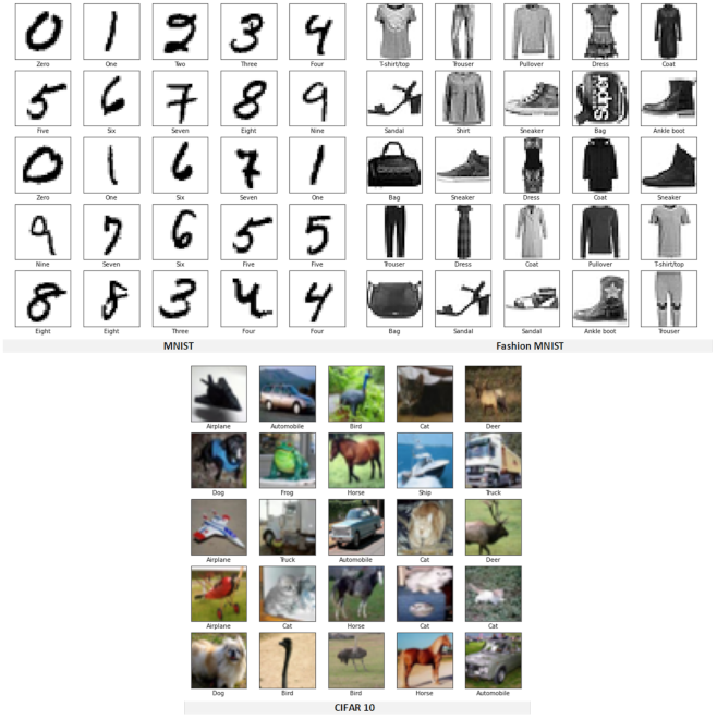
In this section, the three datasets used for experimentation are MNIST, Fashion-MNIST, and the CIFAR-10 datasets.

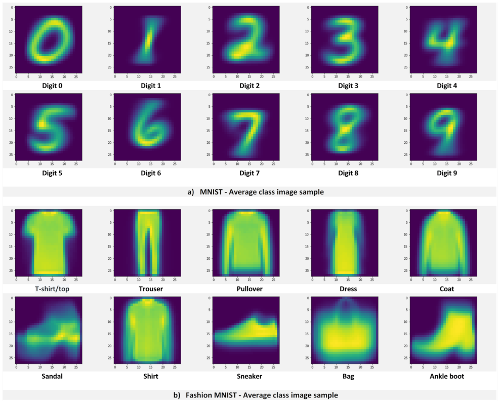
4.1. MNIST

The MNIST database (Modified National Institute of Standards and Technology database) [42] was selected for initial experimentation as it is a commonly used benchmarking dataset in computer vision. The MNIST data is a large dataset of handwritten digits (0–9). The digits are $28\times 28$ pixels in size, greyscale, size-normalized, and centered images.

The MNIST data consist of two parts. The first part contains 60,000 images to be used as training data. The images are scanned handwritten samples from 250 people (from US Census Bureau employees and high school students 50/50). The second part of the MNIST dataset contains 10,000 images from a different set of 250 people to be used as test data.

4.2. Fashion-MNIST

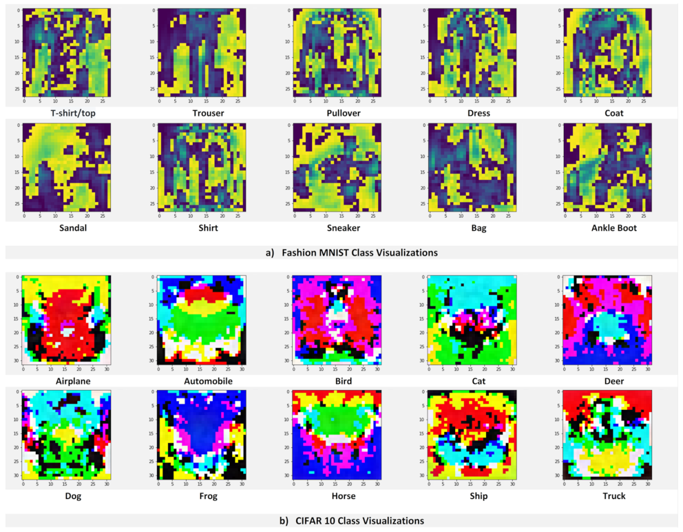
The Fashion-MNIST data is a dataset developed by Xiao et al. [43], for benchmarking computer vision machine learning algorithms. Fashion-MNIST consists of 60,000 training samples and a test set of 10,000 samples. Each sample is a $28\times 28$ grayscale, size-normalized and centered image, paired with a label from 10 classes associated with fashion items (t-shirt/top, trouser, pullover, dress, coat, sandal, shirt, sneaker, bag, and ankle boot). The Fashion-MNIST dataset is intended to serve as a drop-in replacement of the original MNIST data in order to have a more complex dataset for benchmarking machine learning algorithms.

Apart from being common benchmarking datasets, one of the main reasons for selecting the MNIST and Fashion-MNIST datasets was due to their size-normalized and centered qualities. Being size-normalized and centered was helpful during the analysis of the nature of class visualizations, as explained below.

4.3. CIFAR-10

The CIFAR-10 is a labeled subset of the 80 million tiny images in the dataset collected by Alex Krizhevs.ky, Vinod Nair, and Geoffrey Hinton [44]. It is made of 60,000 ($32\times 32\times 3$) color images with 6,000 images per class, belonging to 10 different classes. The data is divided into a training and test set, with 50,000 images for training data and 10,000 test images. The classes in the dataset are completely mutually exclusive and are identified with the following labels: airplane, automobile, bird, cat, deer, dog, frog, horse, ship, and truck.

The CIFAR-10 dataset was selected to validate the results of the experimentation on a harder database with different specifications. Figure 1 shows image samples from the three image datasets used during experimentation.

5. Class Visualizations as Mental Imagery

This section shows the experimentation carried out using class visualizations as training data by considering them analogous to mental imagery.

5.1. Training a Shallow Network Architecture on the MNIST Data

The experimentation began by training a shallow fully connected ANN architecture consisting of only an input and output layer to perform classification on the MNIST dataset. The model was implemented in Google Colaboratory using Python 3 and TensorFlow version 1.15.2.

The network’s specifications are the following:

• 784 input neurons ($28\times 28$ pixels images).
• 10 output neurons with softmax activation function.
• Cross entropy as the cost function to minimize.
• Learning rate = 0.5, minibatch size = 100.

Before training the network, the accuracy of the untrained model was verified to be around 10% (completely random). It will not be mentioned for the remainder of the paper, but every time a new model is trained, its accuracy on untrained weights is verified to be around 10%.

After training the model on the MNIST training data (60,000 images) the accuracy achieved on the test set (10,000 images) was 91.76% accuracy (8.24% error).

Table 1. Confusion Matrix of shallow neural network trained on the MNIST dataset. Correct results are highlighted in bold.

	0	1	2	3	4	5	6	7	8	9
0	963	0	3	2	0	3	6	1	2	0
1	0	1117	2	2	0	2	4	2	6	0
2	8	10	911	17	14	1	12	12	37	10
3	3	2	22	923	0	22	2	10	15	11
4	1	4	2	1	908	0	11	2	5	48
5	9	4	6	46	9	760	18	5	26	9
6	15	3	8	2	11	11	906	1	1	0
7	3	12	20	10	6	1	0	936	3	37
8	9	15	9	31	9	30	11	12	831	17
9	11	8	2	11	27	7	0	18	4	921

shows the confusion matrix for the model trained on the MNIST data, showing the actual class horizontally, and the predicted class vertically.

Table 2. Accuracy metrics of shallow neural network trained on the MNIST dataset.

	0	1	2	3	4	5	6	7	8	9
Precision	0.942	0.951	0.925	0.883	0.923	0.908	0.934	0.937	0.894	0.875
Recall	0.983	0.984	0.883	0.914	0.925	0.852	0.946	0.911	0.853	0.913
F1-Score	0.962	0.967	0.903	0.898	0.924	0.879	0.940	0.924	0.873	0.893
Support	980	1135	1032	1010	982	892	958	1028	974	1009

shows the Precision, Recall, and F1-Score metrics for each class. The Support metric shows the number of occurrences of each label.

5.2. Class Visualization Extraction

Next, one class visualization per class from the trained model was extracted. That is one visualization for each digit (0–9). The task here was to generate an image that best represents a class by finding the image I that maximizes the score $Sc\left(I\right)$, that the ANN assigns to class c. The algorithm starts with a blank image I (all zeros), computes the gradient with respect to I with backpropagation, and makes use of gradient ascent to find a better I. This process is repeated until a local optimum I is found.

Even when the goal is to generate a class visualization that maximizes the output of a particular class, while minimizing the output of the rest, some probabilities for the rest of the classes are always obtained. Therefore, once a class visualization is generated, it is fed to the network, saving the output logits to use as soft targets in the next stage—as soft targets provide more information about the knowledge developed by the underlying model.

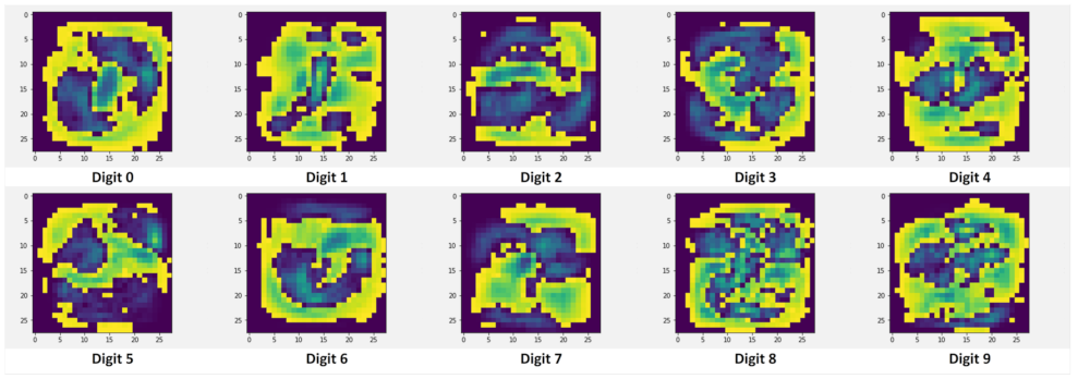
The images shown in Figure 2 were obtained once the class visualization extraction process was complete. The class visualizations vaguely resemble the digit from the class they are representing. Somewhat natural-looking visualizations were obtained thanks to the nature of the dataset (being size-normalized and centered).

Class visualizations give us an insight into what the network is looking for in an image to make a classification. To make the class visualizations more natural-looking, image priors can be included to bias the optimization algorithm. However, since the goal is to validate whether or not class visualizations contain exploitable embedded knowledge—and not the interpretability of the visualizations—image priors were not included.

5.3. Class Visualizations as Training Data

The experimentation continued by training a new network from scratch to perform classification on the MNIST dataset. This network had the same number of layers and neurons; however, the class visualizations previously generated were used as the training set (10 images in total) instead of the 60,000 images from the MNIST training data.

Two other important differences were the use of batch gradient descent and a larger learning rate value, since the 10 class visualizations coupled with soft targets provide more information and less variance in the gradient. Additionally, we do not care about overfitting the training data. In fact, we want to overfit since we are proposing that all the knowledge developed by the first model is contained in the 10 class visualizations.

After training the new network using the class visualizations as training data, the model’s accuracy was calculated on the test set (10,000 images), achieving a 91.62% accuracy (8.38% error). This result shows that, at least for the MNIST dataset and this particular network architecture, class visualizations can function as a compressed version of the original training set, achieving virtually the same accuracy as the original model trained on the MNIST training data (60,000 images). In other words, class visualizations were equivalent to seeing the entire MNIST training data, just as mental imagery resembles the real experience of feeling or perceiving the actual event.

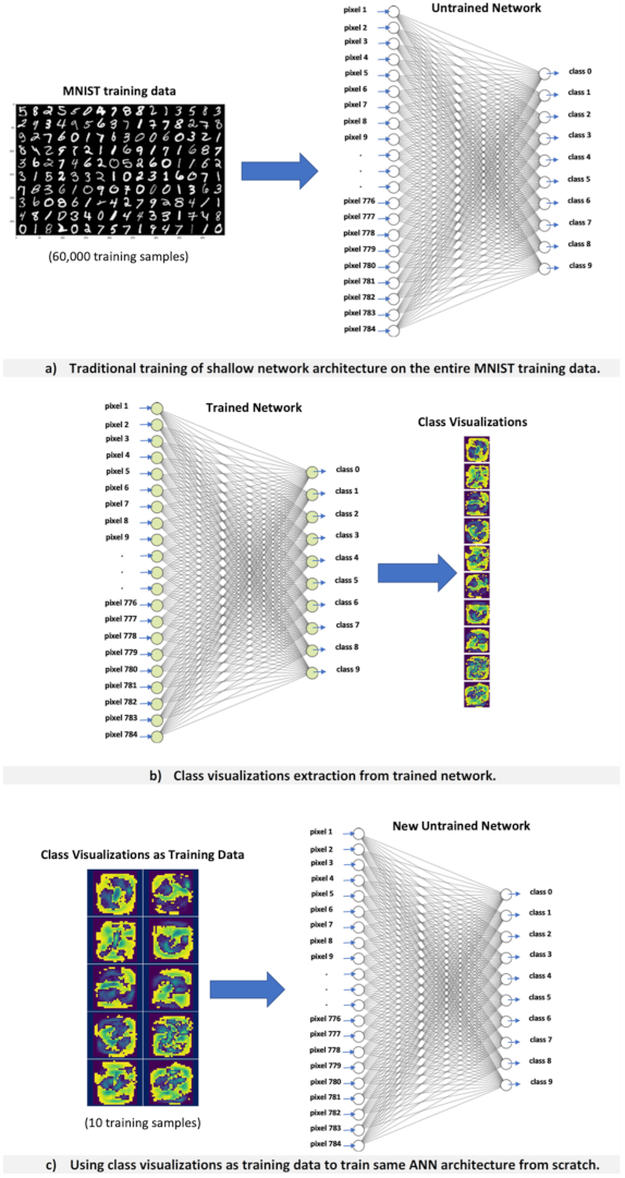
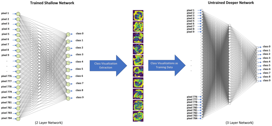
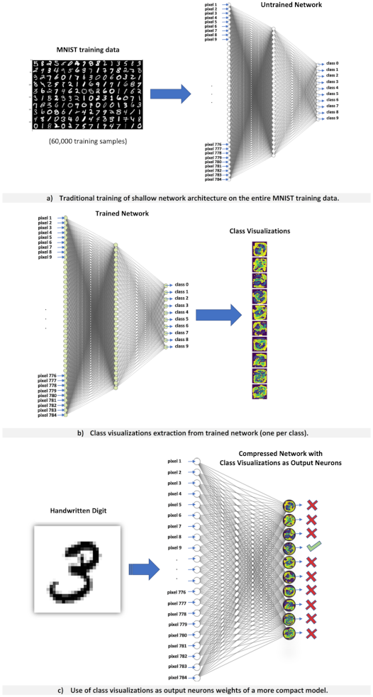
The entire process is shown in Figure 3. Where Figure 3a presents a shallow network architecture trained on the entire MNIST training data in the traditional way. Figure 3b shows the extraction of one class visualization per class, and finally, Figure 3c shows the use of class visualizations as training data to train the same network architecture from scratch.

Table 3. Confusion matrix of shallow neural network trained using class visualizations as training data. Correct results are highlighted in bold.

	0	1	2	3	4	5	6	7	8	9
0	952	0	4	1	1	5	13	1	2	1
1	0	1110	3	2	1	1	4	2	12	0
2	5	12	892	24	13	2	14	13	48	9
3	3	2	20	903	2	18	5	10	35	12
4	0	1	3	1	909	1	12	2	13	40
5	10	3	1	47	13	756	20	3	30	9
6	7	3	5	2	7	12	918	2	2	0
7	3	7	21	7	6	0	0	927	9	48
8	4	11	6	22	8	28	12	5	872	6
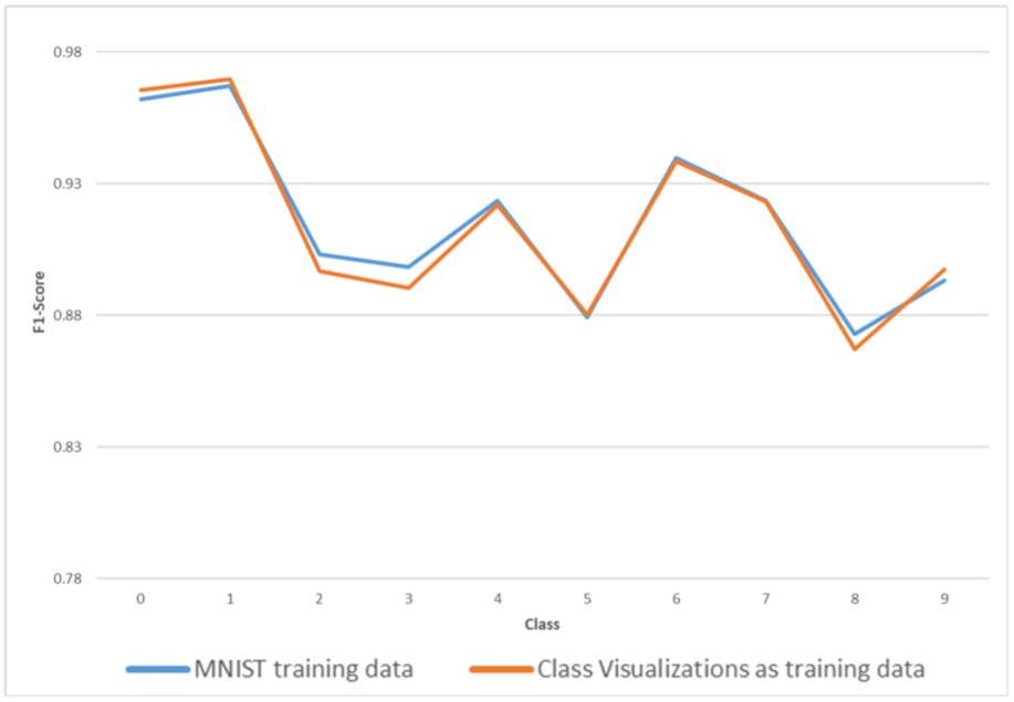
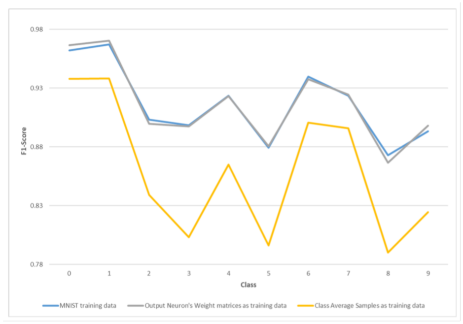
9	8	5	2	9	30	3	0	15	14	923

and

Table 4. Accuracy metrics of shallow neural networks trained using class visualizations as training data.

	0	1	2	3	4	5	6	7	8	9
Precision	0.960	0.962	0.932	0.887	0.918	0.915	0.920	0.946	0.841	0.881
Recall	0.971	0.978	0.864	0.894	0.926	0.848	0.958	0.902	0.895	0.915
F1-Score	0.966	0.970	0.897	0.891	0.922	0.880	0.939	0.923	0.867	0.897
Support	980	1135	1032	1010	982	892	958	1028	974	1009

show the confusion matrix and accuracy metrics of the ANN trained with class visualizations, and Figure 4 shows the F1-Score values of both models to visually compare the two models. It can be seen from Figure 4 and

Table 5. Overall accuracy comparison of different models.

	Trainset	Class Vis.	Class Vis. Deeper	Avg. Images	Output W’s
MNIST	91.76%	91.62%	91.63%	86.02%	91.75%
FMNIST	82.95%	82.01%	82%	75.9%	83.14%
CIFAR10	40.08%	39.65%	38.85%	10%	39.65%

that the performances of both models are very close, almost overlapping, hinting that both models developed the same insights. These results show that we have managed to transfer the knowledge developed by the first model to the second one through class visualizations.

5.4. Repeating the Experiment on the Fashion-MNIST and CIFAR-10 Datasets

To validate the results obtained on the MNIST database, the experimentation was repeated on the Fashion-MNIST and CIFAR-10 datasets. After training a shallow fully connected ANN architecture with no hidden layers on the Fashion-MNIST dataset, the accuracy achieved on the test set was 82.95%. Next, class visualizations from the trained network were extracted. The class visualizations obtained from this network are shown in Figure 5a. After the class visualizations were extracted, they were used to train the same network architecture from the ground up. The accuracy achieved by the new network on the Fashion-MNIST test data was 82.01%; virtually the same accuracy as the one achieved when training the network using all of the Fashion-MNIST training data.

On the CIFAR-10 dataset, a 40.08% accuracy on the test set was achieved after training an ANN architecture with no hidden layers using the CIFAR-10 training data. After extracting one class visualization per class from the trained model and using class visualizations to train the same architecture from scratch, a 39.65% accuracy on the test set was achieved. Figure 5b shows the class visualizations obtained for the CIFAR-10 dataset. Unlike the class visualizations generated from the MNIST and Fashion-MNIST datasets, the visualizations obtained from the CIFAR-10 data do not resemble the classes they represent, however this fact does not seem to matter when using the visualizations to train a new network from scratch.

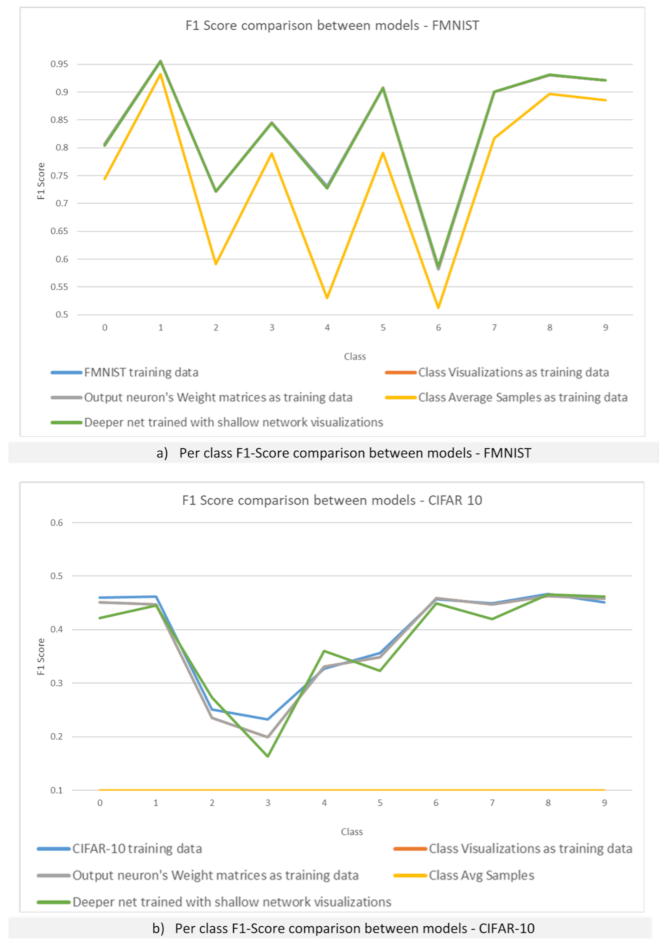
Figure 6a shows a comparison of the F1-Score per class for the network trained on the entire Fashion-MNIST training data versus F1-Score per class for the network trained using class visualizations. Figure 6b shows the same comparison for CIFAR-10. For the Fashion-MNIST classification task, there is a complete overlap between both models, as for CIFAR-10, both models are very close together, almost overlapping as well.

These results further validate the results obtained on the MNIST dataset and the potential for class visualizations to be used as compressed, anonymized versions of the training data. Having a compressed version of the training data would facilitate the distribution of training datasets by providing a compact and anonymized version of the training data.

6. Migrating Class Visualizations from a Shallow to Deeper Network Architecture

To assess whether the use of class visualizations as training data is architecture-dependent, the MNIST class visualizations previously extracted from a shallow network were used to train a slightly deeper network, as shown in Figure 7. The specifications of the deeper architecture are the following:

• 784 input neurons.
• 1 hidden layer with 30 neurons and relu activation function.
• 10 output neurons with softmax activation function.

After using the class visualizations extracted from the shallow network to train this new architecture, the accuracy achieved on the MNIST test set was 91.63% accuracy (8.37% error). Even though class visualizations generated by a different network architecture were used, virtually the same accuracy as the original model is achieved.

Table 6. Confusion matrix of deeper network architecture trained on class visualizations from shallow network. Correct results are highlighted in bold.

	0	1	2	3	4	5	6	7	8	9
0	963	0	2	1	0	3	7	1	3	0
1	0	1114	2	2	0	3	4	1	9	0
2	6	12	892	27	12	1	14	13	47	8
3	3	2	18	918	1	24	4	9	22	9
4	1	2	5	2	914	0	9	1	11	37
5	10	4	4	50	8	759	17	2	32	6
6	13	3	6	2	13	14	903	1	3	0
7	3	10	23	7	8	2	0	931	5	39
8	4	13	5	35	8	25	9	4	862	9
9	9	6	2	15	38	11	0	14	7	907

and

Table 7. Accuracy metrics of deeper network architecture trained on class visualizations from shallow network.

	0	1	2	3	4	5	6	7	8	9
Precision	0.952	0.955	0.930	0.867	0.912	0.901	0.934	0.953	0.861	0.894
Recall	0.983	0.981	0.864	0.909	0.931	0.851	0.943	0.906	0.885	0.899
F1-Score	0.967	0.968	0.896	0.887	0.921	0.875	0.938	0.929	0.873	0.896
Support	980	1135	1032	1010	982	892	958	1028	974	1009

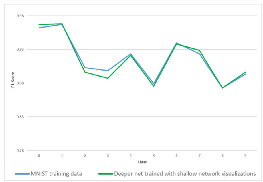
show the confusion matrix and accuracy metrics for this new model. Figure 8 shows that the F1-Score metrics from the shallow network trained using the MNIST training data and the F1-Score metrics obtained from the deeper network trained with class visualizations are very close to one another, almost overlapping, hinting that the deeper network trained with class visualizations developed the same insights as the original model where the class visualizations were extracted from.

These results demonstrate that, at least for this particular case, the use of class visualizations as compressed training data is not restricted to the same network architecture from which they were obtained. The only limitation would be that even when the newer, deeper network has the capacity to achieve better accuracy on the MNIST data, the best accuracy is limited to the accuracy of the model from which the class visualizations were obtained.

Figure 6a,b show that similar results are obtained for both the Fashion-MNIST and CIFAR-10 datasets. Virtually the same accuracy as the model where the class visualizations were extracted is achieved on both datasets when a deeper architecture is trained using class visualizations from a shallow network (82% and 38.85% accuracy, respectively).

7. Class Visualization vs. the Class Average Training Sample

After successfully employing class visualizations as compressed training data, two questions emerged. What exactly do class visualizations represent? Why do visualizations work as a conceptual compression of the training data? Suspicion arose that class visualizations represent the average of all image samples in the training data belonging to a particular class. Given the characteristics of the MNIST database (size-normalized and centered images), this assumption could easily be verified by averaging all the training samples from each class and comparing these class average images against class visualizations.

The images generated for each digit are shown in Figure 9a. These images were obtained after averaging all the training samples per class, as shown in Algorithm 1, and plotting them to visually compare them to class visualizations.

It can be observed from Figure 9a that the class average images are not visually similar to the class visualizations previously obtained. However, even when the class average images are not visually similar to the class visualizations, they may be equivalent in the information embedded within them. To corroborate this, the same shallow network architecture was trained from the ground up, using the class average images as training data.

After training the ANN using the set of class average images, the accuracy of the model on the test data was calculated, achieving 86.02% accuracy (13.98% error).

Table 8. Confusion matrix of shallow network architecture trained using the class average training sample. Correct results are highlighted in bold.

	0	1	2	3	4	5	6	7	8	9
0	921	0	6	9	0	13	19	1	11	0
1	0	1069	8	4	1	7	4	0	42	0
2	7	12	827	70	15	1	25	15	52	8
3	3	2	19	905	1	22	6	12	22	18
4	2	10	5	3	825	1	17	2	22	95
5	12	6	10	119	15	669	15	6	24	16
6	16	4	15	3	13	34	869	0	4	0
7	3	21	28	7	9	0	3	900	16	41
8	4	10	8	105	5	30	13	10	774	15
9	16	10	13	19	42	12	1	35	18	843

and

Table 9. Accuracy metrics of shallow network architecture trained using the class average training samples.

	0	1	2	3	4	5	6	7	8	9
Precision	0.936	0.934	0.881	0.727	0.891	0.848	0.894	0.917	0.786	0.814
Recall	0.940	0.942	0.801	0.896	0.840	0.750	0.907	0.875	0.795	0.835
F1-Score	0.938	0.938	0.839	0.803	0.865	0.796	0.901	0.896	0.790	0.824
Support	980	1135	1032	1010	982	892	958	1028	974	1009

show the confusion matrix and accuracy metrics for the ANN trained using the set of class average images. Figure 10 shows that there is no overlap between the F1-Scores from the model trained on the MNIST data and the model trained using the class average images.

Algorithm 1 Class average Image generation

Require: Training image samples from class C  for each training sample image I in class C do   for each pixel p in image I do    $classAverageImage\left[p\right]$+=$I\left[p\right]$/$\#trainingsamples$   end for  end for

These results show that although the class average images contain exploitable knowledge, it is less than the class visualizations. One possibility for the difference in accuracy could be due to the potential errors in the size-normalization and centering processes. A second possibility for the difference in accuracy is that class visualizations not only contain information about their own class, but also about the other classes, which the model can classify.

Repeating the same experiment on the Fashion-MNIST database obtained similar results. Figure 9b shows the class average images obtained for the Fashion-MNIST database. After generating and using the Fashion-MNIST class average images to train a shallow network, a 75.9% accuracy is achieved, 6.11% lower than the accuracy achieved using class visualizations.

Figure 6a shows that there is no overlap between the F1-Scores from the model trained on the Fashion-MNIST data and the model trained using the class average images. These findings support the results obtained on the MNIST dataset.

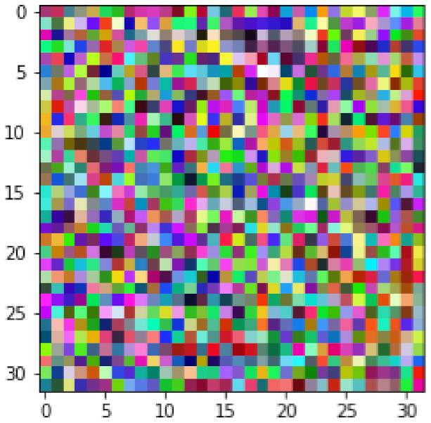
For the case of the CIFAR-10 dataset, this experimentation could not be replicated since the CIFAR-10 training samples are not size-normalized and centered images. Not surprisingly, averaging the training samples from each class yields a noisy image, as shown in Figure 11. Using these images as training data results in a completely random model with an average overall accuracy of 10%.

8. Comparing Class Visualizations Obtained from Different Networks

A new model was trained on only two out of the ten classes from the MNIST database to explore the possibility that the shape of class visualizations—and the knowledge embedded within them—is influenced by the other classes that the model is trained on. For this task, the digits three and four were arbitrarily chosen. The purpose of this experiment was to compare class visualizations for digits three and four taken from a ten-class model that classifies all ten digits (0–9) against visualizations taken from a two-class model that only classifies digits three and four.

The new network architecture to be trained is a shallow architecture without hidden layers and two output neurons—one output neuron for digit three and one for digit four. Therefore, only the training image samples from the MNIST dataset that correspond to those two digits were used as the training data. In the same way, only the validation samples for digits three and four were used to calculate the accuracy of this new model, achieving an overall classification accuracy of 99.7% after training.

Class visualizations for both classes (digits three and four) were generated as before. Next, the class visualizations obtained were used as training data to train the same architecture from scratch. The accuracy achieved using the two class visualizations as training data was 99.7%. In other words, the exact same accuracy was achieved by training the model with class visualizations similar to when all the training data was used. The accuracy achieved shows that the knowledge developed by the first model was successfully extracted into the two class visualizations. The important question now was, are these new class visualizations equivalent to the class visualizations from the 10-class model for digits three and four?

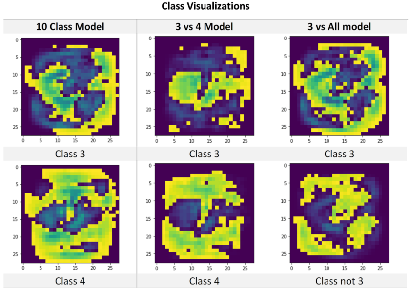
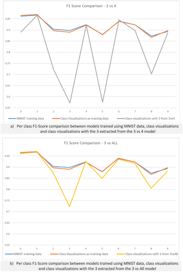
Figure 12 shows that the class visualizations generated for digits three and four from the two-class model (three vs. four models) are visually different from the class visualizations obtained from the 10-class model. These results support the idea that the shape of, and possibly the knowledge embedded in, a class visualization is affected by the other classes that a model is trained on. It was suspected that the more classes a model can classify, the more detail from each class the network needs to learn to differentiate one class from the rest. Therefore, the more difficult the classification task is (i.e., more classes a model can classify), the more detail and embedded knowledge the class visualization will have.

To corroborate this assumption, the set of class visualizations obtained from the 10-class model were taken, swapping the class visualization of digit three with the class visualization of digit three from the 2-class model. The new set of ten class visualizations was used as training data to train a new 10-class model from scratch, achieving a classification accuracy of 80.39% on the validation set. The performance achieved was considerably lower from the accuracy obtained by training the same architecture with the original 10-class visualizations (91.76% accuracy).

Table 10. Confusion Matrix of shallow neural network trained on class visualizations taken from the 10-class model with the visualization of digit three swapped with the class visualization obtained from the three vs. four model. Correct results are highlighted in bold.

	0	1	2	3	4	5	6	7	8	9
0	811	0	2	152	0	1	10	0	2	2
1	0	1092	0	32	0	1	3	2	5	0
2	2	6	605	359	12	0	11	10	14	13
3	0	1	7	985	2	3	1	2	3	6
4	2	1	4	0	901	0	9	3	7	55
5	7	3	1	445	15	369	16	5	21	10
6	7	3	4	12	9	4	915	3	1	0
7	2	5	12	82	4	0	0	870	3	50
8	3	8	6	335	11	12	12	5	559	23
9	6	6	2	30	20	1	0	10	2	932

shows the confusion matrix for this new model. As expected, the confusion matrix shows that the decrease in accuracy was caused by an increase in false positives (shown in red) for the digit three class. These results point to the class visualization of digit three as the most likely culprit for the decrease in accuracy.

It can be observed that for digit three, the number of false positives when the digit was actually a four is zero. This suggests that the class visualization of digit three has embedded knowledge to help differentiate a three from a four but lacks the knowledge to differentiate a three from the rest of the digits, resulting in high false positives for the other classes (if the digit is not a four, it must be a three).

To further confirm these results, a new 2-class model to classify the digit three against any other digit was trained (three vs. All model). By increasing the difficulty of the classification task, the generation of a more detailed, and more (embedded) knowledgeable class visualization of the digit three was expected.

A new model using all of the MNIST training samples corresponding to digit three and a subset of the rest of the digits (to have a balanced dataset) was trained; achieving a classification accuracy of 97.82% on the test set after training. Next, class visualizations for each of the two classes (class three and not class three) were extracted from the model. In order to verify the quality of the visualizations generated, the two class visualizations were used to train the same architecture from scratch, achieving a 97.39% accuracy. The class visualizations obtained from the network are shown in Figure 12 (three vs. All model). It can be observed that this new class visualization, of digit three, is visually more similar to the visualization of digit three from the 10-class model.

Next, a new 10-class model was trained using the original ten class visualizations extracted from the 10-class model, swapping the visualization of digit three with the visualization of the digit three from the three vs. All model. After training, a classification accuracy of 88.78% on the MNIST validation set was achieved. This accuracy is closer to the original accuracy achieved with the original 10 class visualizations.

Table 11. Confusion matrix of shallow neural network trained on the class visualizations taken from the 10-class model with the class visualization of digit three swapped with the class visualization obtained from the three vs. All model. Correct results are highlighted in bold.

	0	1	2	3	4	5	6	7	8	9
0	955	0	2	0	0	4	11	1	6	1
1	0	1108	4	0	0	1	4	2	15	1
2	7	12	903	1	9	2	17	15	58	8
3	12	2	69	576	2	103	13	19	174	40
4	2	1	9	0	890	0	7	3	19	51
5	11	4	4	5	6	770	20	3	53	16
6	7	3	5	0	7	13	916	3	4	0
7	3	7	26	1	5	0	0	934	12	40
8	4	11	6	1	4	23	12	5	902	6
9	8	5	2	0	19	4	0	23	24	924

shows the confusion matrix for this new model. This time, the number of false negatives (shown in red) increased and the number of false positives for class three decreased, showing that training with this new class three visualization forces the network to be more careful when classifying a digit as three.

Figure 13 presents a comparison of the F1-Score metrics for the models trained in this section. These results show that the increased difficulty of differentiating the digit three from any other digit produced a better-quality class visualization with more embedded knowledge. This supports the notion that class visualizations not only contain information about their class, but also about the other classes that the network can classify.

9. Visualizations of Output Neurons vs. Class Visualizations

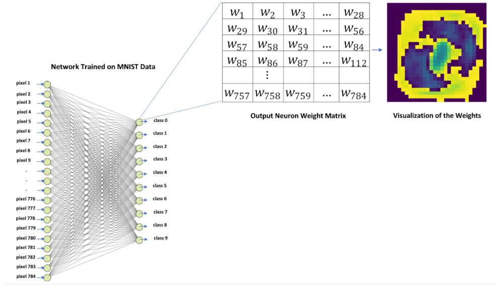
After validating that class visualizations do not correspond to the class average training sample, it was suspected that a class visualization could be analogous to the compression of all the weights in the network that are relevant for the classification of a particular class. Given the simple architecture of our network for the classification of the MNIST data (no hidden layers), identifying the weights that are relevant to the activation of a particular class can be done in a straightforward way—using only the weights of the output neuron of the class in question.

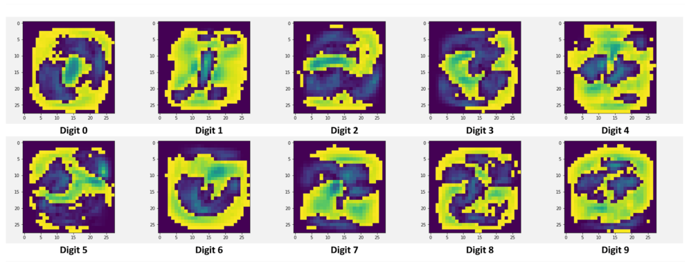
To verify this premise, the weight matrix of each output neuron was taken and plotted as a $28\times 28$ image by treating the weight values as pixel intensities, as shown in Figure 14. The images obtained after plotting the weight matrices of the output neurons are shown in Figure 15.

It can be observed from the images shown in Figure 15 that the weight matrices of the output neurons plotted as images look very similar to the class visualizations obtained at the first stages of experimentation.

In order to verify how analogous the weight matrices of the output neurons are to the class visualizations, a new shallow ANN was trained from scratch, using the weight matrices of the output neurons as training data. After training this new model, the best accuracy achieved on the test set was 91.75% (8.25% error). At this point, we must emphasize that the accuracy achieved by using the weight matrices of the output neurons as training data was virtually the same accuracy as the one obtained using class visualizations as training data, or when the entire MNIST training set was used.

Table 12. Confusion matrix of shallow neural network trained on class visualizations made from weight matrices of output neurons. Correct results are highlighted in bold.

	0	1	2	3	4	5	6	7	8	9
0	955	0	2	1	1	5	12	1	2	1
1	0	1113	2	2	0	1	4	2	11	0
2	4	12	898	19	13	3	15	9	50	9
3	3	2	20	900	2	19	5	9	38	12
4	1	1	4	1	910	0	11	0	14	40
5	10	4	1	41	11	752	22	3	38	10
6	8	3	5	3	9	11	917	0	2	0
7	3	8	24	5	7	0	0	917	12	52
8	4	11	6	18	7	23	12	2	884	7
9	8	5	2	6	29	2	0	13	15	929

and

Table 13. Accuracy metrics of shallow neural network trained on class visualizations made from weight matrices of output neurons.

	0	1	2	3	4	5	6	7	8	9
Precision	0.959	0.960	0.932	0.904	0.920	0.922	0.919	0.959	0.829	0.876
Recall	0.974	0.981	0.870	0.891	0.927	0.843	0.957	0.892	0.908	0.921
F1-Score	0.967	0.970	0.900	0.897	0.923	0.881	0.938	0.924	0.867	0.898
Support	980	1135	1032	1010	982	892	958	1028	974	1009

show the confusion matrix and accuracy metrics of the new model.

It can be observed in Figure 10 that the F1-Score metrics from the shallow network trained on the MNIST training data and the metrics from the network trained using the weight matrices as training data are very close to one another. Additionally, Table 5 shows that the overall accuracy from the model trained using class visualizations and the accuracy from the model trained using the weight matrices as training data are very close to one another. This hints at the possibility of class visualizations being equivalent to a compression of all weights in the network that are important for the activation of a particular class.

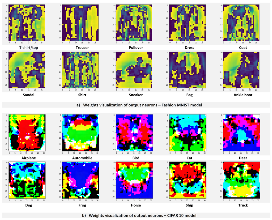
For the Fashion-MNIST and CIFAR-10 datasets, similar results were obtained. Figure 16 shows the visualizations of the output weight matrices of a shallow network architecture trained on the Fashion-MNIST and the CIFAR-10 data, respectively. As with the MNIST data, the visualizations of the output weight matrices, for both Fashion-MNIST and CIFAR-10, look very similar to the class visualizations obtained from their respective networks.

Figure 6a shows that, for the Fashion-MNIST dataset, training the same model from scratch using the visualizations of the output weight matrices as training data, yields exactly the same accuracy as when using the entire training data or class visualizations, achieving 83.14% accuracy on the test set. Similar results were obtained for the CIFAR-10 dataset. Training the same model from scratch using the visualizations of the output weight matrices as training data achieves the same performance as training the model using class visualizations, 39.65% accuracy. These results are shown in Figure 6b.

The obtained results are quite significant. If, in fact, class visualizations represent all the weights in the network that are important for the activation of a particular class then, correctly extracted visualizations from an ANN could potentially be used as convolutional filters for extreme model compression purposes. Extreme model compression using class visualizations could potentially be accomplished by employing class visualizations as output neurons of a compact model, leaving only the biases of the output neurons to be trained.

10. Class Visualizations and Model Compression

After achieving results suggesting that visualizations of the output neuron weights are analogous to class visualizations in shallow architectures without hidden layers, experimentation with class visualizations for model compression purposes followed.

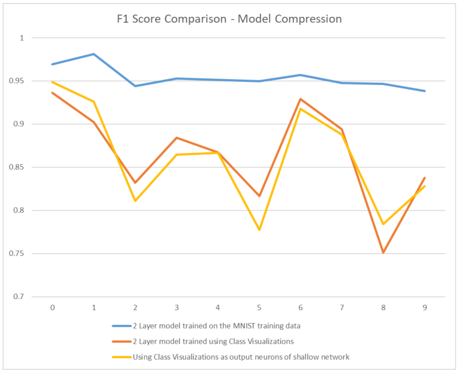
Experimentation started by training a three-layer neural network (784 input layer, 30 neurons hidden layer, 10 neurons output layer) on the MNIST training data (60,000 training samples), achieving an accuracy of 95.42% on the MNIST test set after training. Proceeding with the generation of one class visualization per class as previously done, via class maximization and backpropagation to the input, they were run through the network to generate soft target labels. Having generated 10 class visualizations (one per class), they were used as training data to train the same network architecture from scratch.

After training the same model from the ground up using class visualizations, an overall accuracy of 86.38% was achieved on the MNIST test set. The decrease in accuracy is believed to be due to the need of more than just one class visualization per class to successfully extract all the knowledge developed by the model. Having a network with more than one layer means that the model can generate more than one “mental image” per class. This is because, more than one combination of the 30 neurons in the hidden layer could be possible for the activation of a particular class. Therefore, a more robust approach would be needed to generate all the class visualizations that are required to extract all the knowledge that deeper networks develop. This will remain for future work.

Next, the ten class visualizations obtained were used to attempt the transfer of the knowledge embedded in them to a more compact network—an ANN with ten output neurons and no hidden layers. The goal here was to transfer the 86.38% accuracy achieved when using the class visualizations as training data to a more compact model. To achieve this, each class visualization was taken and placed as the weight matrix of an output neuron of the compact model.

Only the task of training the biases of the output neurons (10 biases) remained. To train the biases, all the network’s weights were frozen and the MNIST training data was used to train the biases via backpropagation. After training the biases, the accuracy achieved on the MNIST test data was 86.38%, which is exactly the same accuracy achieved when using the ten class visualizations to train the deeper network. It is important to note that this accuracy was achieved after training only 10 parameters of the network (10 biases). Figure 17 shows that the F1-Score metrics from the shallow network that uses class visualizations as convolutional filters and the F1-Score metrics obtained from the deeper network trained with class visualizations are very close to one another.

The results obtained in this section show that class visualizations have the potential to be used for extreme model compression purposes, by using class visualizations as convolutional filters of a more compact network. Although, the development of techniques to extract all the knowledge developed by deeper architectures into class visualizations is required, the fundamentals of how model compression could potentially be implemented using class visulizations is presented here. Figure 18 shows the approach followed in this section for the use of class visualizations for model compression purposes.

11. Conclusions and Future Work

The main contribution of this paper is showing that class visualizations are not just visual aids that provide insights on what an ANN is looking for. We show that class visualizations contain actual embedded knowledge that can be exploited in a more automatic manner by considering them analogous to mental imagery in humans.

By considering class visualizations analogous to mental imagery, they can be used as a conceptual compression of the entire training data. Having a highly compressed, conceptual version of the training data enables the distribution of training datasets in a compact and anonymized way, providing confidentiality to the data being shared while facilitating its distribution.

Another important contribution of this paper is providing insights into the nature of class visualizations. We demonstrate that a class visualization is not equivalent to the class average training sample and that its shape and embedded knowledge is not only influenced by the training samples from its own class, but by the other classes that the network is trained on as well.

We show that class visualizations are analogous to the visualization of the weight matrices of the output neurons in shallow architectures without hidden layers. Finally, we demonstrate that class visualizations can be used as convolutional filters and show how class visualizations could potentially be used for extreme model compression.

In general, the main focus of this paper is to explore the nature of class visualizations to gain a better understanding of the knowledge embedded in them and to experiment with potential applications of class visualizations. While we show the potential of class visualizations for dataset and model compression, more work is needed on these topics. However, the fundamentals regarding implementation are presented here.

Future work will focus on developing more robust and generalized methods that can be applied on a wide variety of network architectures and data, to enable the extraction of class visualizations for dataset and model compression purposes. In particular, we are beginning experimentation with the use of autoencoders to generate class visualizations directly from training data, without first needing to train a classification network.