Article

A Satellite Incipient Fault Detection Method Based on Local Optimum Projection Vector and Kullback-Leibler Divergence

1
Innovation Academy for Microsatellites of CAS, Shanghai 201203, China
2
University of Chinese Academy of Sciences, Beijing 100049, China
3
School of Information Science and Technology, ShanghaiTech University, Shanghai 201210, China
*
Author to whom correspondence should be addressed.
Appl. Sci. 2021, 11(2), 797; https://doi.org/10.3390/app11020797
Submission received: 30 November 2020 / Revised: 10 January 2021 / Accepted: 10 January 2021 / Published: 15 January 2021
(This article belongs to the Special Issue Machine Fault Diagnostics and Prognostics II)

Abstract

:
Timely and effective detection of potential incipient faults in satellites plays an important role in improving their availability and extending their service life. In this paper, the problem of detecting incipient faults using projection vector (PV) and Kullback-Leibler (KL) divergence is studied in the context of detecting incipient faults in satellites. Under the assumption that the variables obey a multidimensional Gaussian distribution and using KL divergence to detect incipient faults, this paper models the optimum PV for detecting incipient faults as an optimization problem. It proves that the PVs obtained by principal component analysis (PCA) are not necessarily the optimum PV for detecting incipient faults. It then compares the on-line probability density function (PDF) with the reference PDF for detecting incipient faults on the local optimum PV. A numerical example and a real satellite fault case were used to assess the validity and superiority of the method proposed in this paper over conventional methods. Since the method takes into account the characteristics of the actual incipient faults, it is more adaptable to various possible incipient faults. Fault detection rates of three simulated faults and the real satellite fault are 98%, 84%, 93% and 92%, respectively.

1. Introduction

Some faults may occur during the operation of satellites because of the uncertainties of the space environment, the limitations on pre-launch testing, and the imperfect design of satellites. It remains a challenge to detect and solve incipient faults and avoid further complications [1,2]. At present, the detection of faults in satellites is done by comparing the telemetry parameters with the preset thresholds [3,4]. However, this method is not suitable for detecting incipient faults because they may not change significantly during early manifestation of the fault. Compared to system signals, the amplitudes of incipient faults are small, typically from 1 to 10% [5,6] and can easily be masked by the normal variations in systems [7].
Model-based fault detection methods have the advantage of being highly intelligent and interpretable. Examples of such systems include the Livingstone2 and the HyDE fault diagnosis models developed by National Aeronautics and Space Administration (NASA) [8] as well as the Testability Engineering and Maintenance System (TEAMS), developed by Qualtech Systems Inc (QSI) [9]. All of these model-based fault detection methods require manual fault modeling by experts in the field. In addition, the accuracy of these models has a determining impact on their final performance at detecting faults. However, due to the high cost yet low yield of components used in satellites, the lifetime tests or the acquisition of actual fault samples required to build accurate models may often be too costly. Moreover, model-based fault detection methods are only capable of detecting a narrow range of faults. This means that there may be faults that occur outside of the range detectable by the models and this may result in undetected incipient faults [10].
In recent years, data-driven fault detection methods have become a popular field of research [11,12,13]. These methods effectively utilize the extensive ground test data and operational data of satellites, with limited involvement of experts and do not require accurate mathematical models. Iverson et al. [14] proposed a fault detection method named the Inductive Monitoring System (IMS) and used it to detect faults in the Columbia Space Shuttle, and the TacSat-3 satellite. Schwabacher et al. [15] compared four data-driven fault detection methods containing IMS and One Class Support Vector Machine (OS-SVM). Pang et al. [16] proposed a fault detection method based on Gaussian Process Regression (GPR) and implemented it to detect faults in the periodic telemetry parameters of satellites [16]. Hundman et al. [17] proposed a spacecraft fault detection method based on Long Short-Term Memory (LSTM) networks and dynamic thresholds. Tariq et al. [18] proposed a fault detection method using a combination of multivariate convolutional LSTM and probabilistic principal component analysis (PCA) and applied it to the Korea Multi-Purpose Satellite 2 (KOMPSAT-2). Among these data-driven fault detection methods, distance-based fault detection methods such as IMS and OS-SVM are suitable for detecting fault data that are significantly different from normal data. However, these methods are less effective when the fault data and normal data mostly overlap. The fault detection methods using GPR or LSTM are suitable for detecting faults in regular (e.g., periodic) and time-continuous systems, but are ineffective when the telemetry parameters include interruptions in time.
Among the data-driven fault detection methods, methods based on PCA rely on the simplicity of the principle and on good real-time performance and have been used extensively in detecting faults in equipment [19,20]. The Hotelling’s T 2 and squared prediction error (SPE) statistic are usually used to measure deviations in the principal subspace, and to measure deviations in the residual subspace, respectively. However, the conventional T 2 and SPE statistics are not effective at detecting incipient faults that are easily drowned out by noise [21]. Jinane et al. [21] proposed an incipient fault detection method using Kullback-Leibler (KL) divergence and PCA. On the basis of Jinane et al.’s research, Chen et al. [22] proposed an improved method. The proposed method monitors the derivations in principal and residual subspace. Youssef et al. [23] investigated a method of setting the threshold for fault detection using KL divergence for unknown distribution.
However, existing methods for detecting incipient faults based on PCA and KL divergence depend entirely on the off-line normal data to obtain the principal components. Each principal component is essentially a projection vector (PV). Once the normal data have been determined, the PVs used to detect faults also remain fixed. Unfortunately, the PVs obtained by PCA are not necessarily the optimum PV to detect the incipient fault from the view of fault detection. Fixed PVs may result in lower fault detection rates for some types of incipient faults [24,25]. To address the problem of detecting incipient faults in satellites, this paper proposes a novel incipient fault detection method based on local optimum PV (LOPV) and KL divergence. The main contributions of the present research are summarized in the following three points:
  • This paper puts forward the argument that the PVs obtained by PCA are not necessarily the optimum PV for using KL divergence to detect an incipient fault.
  • The problem of finding the optimum PV to detect the incipient fault is modeled as an optimization problem, and the KL divergence is used to detect the incipient fault on the LOPVs.
  • The application of the incipient fault detection method based on PCA and KL divergence is extended to the satellites. The effectiveness of the proposed method is proven in a real satellite fault.
This paragraph outlines the structure of this paper. Section 2 provides a brief introduction about PCA and KL divergence. In Section 3, the incipient fault detection method based on LOPV and KL divergence is presented in detail. In Section 4, the proposed method is validated and analyzed by using a numerical example and a real satellite fault. Finally, the conclusions are presented in Section 5.

2. Preliminary

2.1. PCA

Let n 0 , m be the numbers of samples and variables of a normal data matrix X R n 0 × m ,with X = [ x 1 , , x k , , x m ] . In general, each column of the original normal data X is standardized to eliminate the impact of different ranges of variables.
x ¯ k = x k E ( x k ) σ ( x k ) , k [ 1 , m ]
E ( x k ) and σ ( x k ) in Equation (1) are the mean and standard deviation of the kth column in the matrix X , respectively. The covariance matrix Σ R m × m of the standardized normal data matrix X ¯ is then extracted and the singular value decomposition (SVD) is performed.
Σ = X ¯ T X ¯ n 0 1 = V Λ V T = [ P P ] [ Λ p c 0 0 Λ r e s ] [ P P ] T
The matrix V = [ v 1 , , v m ] R m × m in Equation (2) is a set of standard orthogonal bases in R m space. The space P = [ v 1 , , v l ] R m × l consists of the first l column vectors in the matrix V , is the principal component subspace, and the space P = [ v l + 1 , , v m ] R m × ( m l ) which consists of the last m l column vectors is the residual subspace [26].
The PCA based fault detection method usually uses the two statistics T 2 and SPE, for fault detection. The calculations of the T 2 statistic and the SPE statistic are shown in Equations (3) and (4), respectively. A fault is considered to have occurred when either the T 2 or the SPE statistic has exceeded its corresponding detection threshold of δ T 2 or δ S P E 2 , respectively [27].
T 2 = Λ p c 1 2 P T X ¯ T 2 δ T 2
S P E = X ¯ ( I m × m P P T ) X ¯ T δ S P E 2

2.2. KL Divergence

KL divergence is often used to measure the difference between two probability distributions in the same event space and is widely used for optimization tasks in machine learning [28,29]. The KL divergence between two continuous probability density functions (PDFs) f 1 and f 2 is defined as follows [30]:
I ( f 1 f 2 ) = f 1 ( x ) log f 1 ( x ) f 2 ( x )
Since the above definition does not satisfy symmetry and may result in I ( f 1 f 2 ) I ( f 2 f 1 ) , an improved form of KL divergence referred to as symmetric KL divergence is presented as follows [21]:
K L D ( f 1 f 2 ) = I ( f 1 f 2 ) + I ( f 2 f 1 )
Let n 1 , m be the numbers of samples and variables of on-line data matrix Y R n 1 × m . The main processes of the conventional incipient fault detection methods based on PCA and KL divergence are as follows [21,22]:
  • The standardized normal data X ¯ are projected on each PV v j and the reference PDF of the normal data is obtained after projection on v j as f j and the corresponding detection threshold is ε j , v j V , j [ 1 , m ] .
  • Each column y k of the on-line data matrix Y is standardized with y ¯ k = y k E ( x k ) σ ( x k ) , k [ 1 , m ] .
  • The standardized on-line data Y ¯ are projected on each PV v j to obtain the PDF g j of the on-line data.
  • Equation (6) is used to calculate the KL divergence K L D ( f j | | g j ) between the PDF g j and the reference PDF f j for each PV v j .
  • Whether the K L D ( f j | | g j ) is greater than the corresponding detection threshold ε j is determined for each PV v j . It is considered to be faulty when at least one of the m units of K L D ( f j | | g j ) exceeds the corresponding detection threshold.
    { H 0 : v j , v j V , K L D ( f j | | g j ) ε j , fault - free H 1 : v j , v j V , K L D ( f j | | g j ) > ε j , faulty

3. Incipient Fault Detection Method Based on LOPV and KL Divergence

For each PV v j , if the fault detection method could detect an incipient fault with a high detection rate on the v j , then v j is considered sensitive to the incipient fault with a given significance level α . The bigger the detection rate, the greater sensitivity to the incipient fault. It can be seen from formula (7) that the incipient fault can be well detected if there is one PV sensitive to the fault. From the perspective of fault detection, we hope to find an optimum PV that is most sensitive to the incipient fault.

3.1. Optimum PV for Incipient Fault Detection

We assume that there is an optimum PV that is more sensitive to the incipient fault than the existing PVs v 1 , v 2 , , v m and the optimum PV is w R m . To find the optimum PV, this paper assumes the m dimensional feature parameters to be monitored in their normal state, obeying the m dimensional joint Gaussian distribution X R n 0 × m ~ N ( μ x , Σ x ) . Let the projection of X on w be F R n 0 . By the nature of the m dimensional joint Gaussian distribution, F obeys the one-dimensional Gaussian distribution F ~ N ( μ x T w , w T Σ x w ) [26].
F = X w = x 1 w 1 + x 2 w 2 + + x m w m
We assumed that after the incipient fault occurs, the on-line faulty data Y still obey the m dimensional joint Gaussian distribution Y R n 1 × m ~ N ( μ y , Σ y ) . However, due to the fault, the mean vector μ y R m and the covariance matrix Σ y R m × m of Y deviated and that their deviations were Δ μ and Δ Σ , respectively.
μ y = μ x + Δ μ
Σ y = Σ x + Δ Σ
The projection of Y on w is G = Y w . Then, from the nature of the joint Gaussian distribution, G obeys the one-dimensional Gaussian distribution G ~ N ( μ y T w , w T Σ y w ) . Assume that there are two PDFs f and g for two Gaussian distribution signals F ~ N ( μ 1 , σ 1 2 ) and G ~ N ( μ 2 , σ 2 2 ) , respectively. The KL divergence of f and g can be expressed as follows [21]:
K L D ( f | | g ) = 1 2 [ σ 2 2 σ 1 2 + σ 1 2 σ 2 2 + ( μ 1 μ 2 ) 2 ( 1 σ 1 2 + 1 σ 2 2 ) 2 ]
The projections of the normal data matrix X and the faulty data matrix Y on w obey the one-dimensional Gaussian distribution F ~ N ( μ x T w , w T Σ x w ) and G ~ N ( μ y T w , w T Σ y w ) , respectively. Consequently, the mean and variance of F and G can be brought into Equation (11), respectively, obtaining:
K L D ( f | | g ) = 1 2 [ w T Σ y w w T Σ x w + w T Σ x w w T Σ y w + ( μ x T w μ y T w ) 2 ( 1 w T Σ x w + 1 w T Σ y w ) 2 ] = 1 2 [ w T Σ y w w T Σ x w + w T Σ x w w T Σ y w + ( Δ μ T w ) 2 ( 1 w T Σ x w + 1 w T Σ y w ) 2 ]
In Equation (12), the mean deviation vector Δ μ , normal data covariance matrix Σ x , and on-line faulty data sample covariance matrix Σ y can be obtained through the on-line faulty data matrix Y and normal data matrix X . Therefore, when historical normal data X and the on-line faulty data Y to be verified are obtained, only the PV w is unknown in Equation (12). In other words, K L D ( f | | g ) is a function h ( w ) on the PV w as shown in Equation (13).
h ( w ) = K L D ( f | | g ) = 1 2 [ w T Σ y w w T Σ x w + w T Σ x w w T Σ y w + ( Δ μ T w ) 2 ( 1 w T Σ x w + 1 w T Σ y w ) 2 ]
Sliding windows with the length of n 1 are used to divide the normal data matrix X and submatrices of X can be obtained X 1 , , X i , , X r , X i R n 1 × m , i [ 1 , r ] . We project all submatrices X 1 , , X i , , X r on w to obtain r PDFs P D F X 1 , , P D F X i , , P D F X r . We assume that each P D F X i obeys a one-dimensional Gaussian distribution. The KL divergence between P D F X i and f can be calculated by Equation (13). h X i ( w ) = K L D ( f | | P D F X i ) , i [ 1 , r ] . The process used to obtain vector h X ( w ) is shown in Figure 1.
h X ( w ) = [ h X 1 ( w ) , , h X i ( w ) , , h X r ( w ) ]
J ( w ) = h ( w ) E ( h X ( w ) ) σ ( h X ( w ) )
The relative deviation in KL divergence of the on-line faulty data matrix Y and normal data matrix X on the PV w is defined as shown in Equation (15). E ( h X ( w ) ) and σ ( h X ( w ) ) in Equation (15) are the mean and standard deviation of the vector h X ( w ) . E ( h X ( w ) ) and σ ( h X ( w ) ) reflect the center and range of the interval of variation range of the KL divergence for normal data after projection on w , respectively. Once the on-line faulty data matrix Y and normal data matrix X are given, the KL relative deviation J ( w ) still remains as the function about w .
With the given significance level α , the matrix Y and the matrix X , The larger the value of the J ( w ) , the easier it is for that fault to be detected. On the contrary, if the value of the J ( w ) is small, it is likely to be drowned out by the noise and this leads to poor performance in detection of the fault. Thus, the problem of finding the optimum PV for fault detection can be modeled as an optimization problem, as shown in Equation (16).
{ min w J ( w ) s . t . w T w = 1 ; w i , 1 w i 1 , i [ 1 , m ]
If the PV w is directly optimized in Equation (16) so that h ( w ) is maximized, and the optimum solution may continue to converge on the PV corresponding to the smallest eigenvalue, thus making the optimization process meaningless. The above mentioned problem arises because the variation ranges of the eigenvalues of the different PVs are different. A small eigenvalue leads to small w T Σ x w and w T Σ y w in Equation (13), which are exactly in the denominator position, and slight noise can cause large fluctuations in the KL divergence on the corresponding PVs of the small eigenvalue. Therefore, it is necessary to standardize h ( w ) , and the optimization goal is to maximize the relative deviation of KL divergence, J ( w ) , rather than the absolute deviation of KL divergence, h ( w ) .
The goal of PCA is to maximize the variance of the normal data X after it is projected on the PV w and can be modeled as an optimization problem, as shown in Equation (17) [26].
{ min w w T Σ x w s . t . w T w = 1
We supposed that w p is the optimum solution of the optimization problem shown in formula (16), w q is the optimum solution of the optimization problem shown in formula (17). Since the objective functions of the two optimization problems are different, w T Σ x w J ( w ) , generally, w p is not equal to w q . However, solving formula (16) solves the optimization problem, and w p is the optimum PV for using KL divergence to detect the fault. Because w p w q , w q is not the optimum PV for using KL divergence to detect a fault in general. Therefore, the PVs obtained by PCA are not necessarily the optimum PV for using KL divergence to detect the fault.
Equation (16) converts the problem of finding the maximum J ( w ) into a standard constrained optimization problem by adding a negative sign and constrained conditions. The search for the optimum PV w that maximizes J ( w ) is on the surface of a hypersphere with a radius of 1. Equation (16) is a typical constrained optimization problem, which can be solved using readily available tools for solving optimization problem, such as the fmincon function built into MATLAB 2019b.
Since the objective function min w - J ( w ) in Equation (16) is a nonlinear function about w , the solution obtained by the iterative method is not necessarily a global optimum solution, but probably a local optimum solution [31,32]. However, considering that the optimization problem shown in Equation (16) needs to be solved when each set of on-line data arrives, finding the global optimum solution will undoubtedly increase the computational cost. Considering the timeliness, the iteration can be stopped when the optimization problem in Equation (16) converges to a local optimum solution that is better than the existing fixed PVs.
It is necessary to ensure that the local optimum solution searched for by Equation (16) is better than all the fixed PVs of v 1 , v 2 , , v m obtained by PCA. To achieve this, when the on-line data Y arrive, the on-line data Y are projected on each fixed PV v 1 , v 2 , , v m and the mean value drift vector μ , respectively. The KL divergence relative deviations are calculated according to Equations (13)–(15) in each PV and the vector of mean value drift. Then the vector v j that makes the largest KL divergence relative deviation is selected as the initial iteration vector w 0 of the optimization problem in Equation (16).
{ w 0 = v j s . t . J ( v j ) = max ( J ( v 1 ) , J ( v 2 ) , , J ( v m ) , J ( v m + 1 = Δ μ Δ μ ) ) , j [ 1 , m + 1 ]

3.2. Detecting Incipient Faults Using LOPVs and Dynamic Thresholds
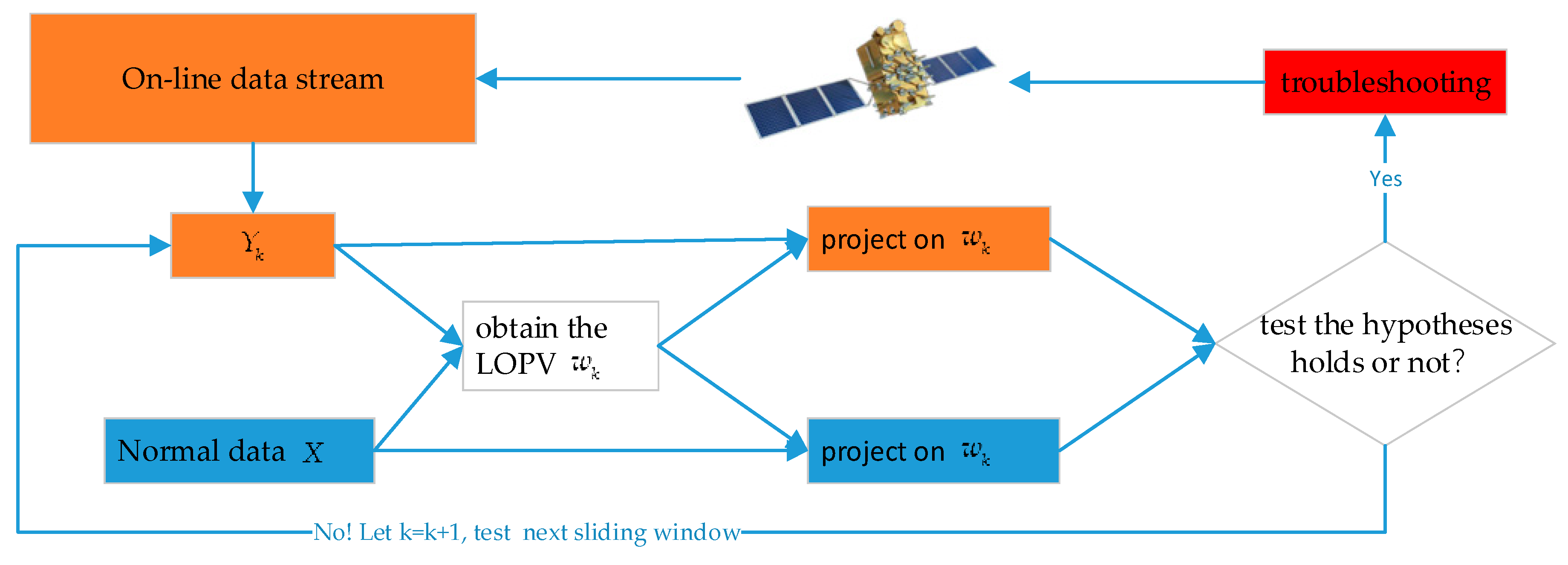
In this section, sliding windows with the length of n 1 are used to extract and monitor the on-line data in real time. The on-line data extracted by the k t h sliding window are Y k R n 1 × m . This article intends to use the idea of hypothesis testing to detect incipient faults for each Y k , as shown in Figure 2. Let us assume that Y k is faulty, then we test this hypothesis holds. If the hypothesis held after testing, it is considered that a fault has occurred in Y k . Otherwise, Y k is normal. The specific hypothesis testing steps are as follows:
  • Let Y = Y k , we assume that Y k is faulty. The method is used as described in Section 3.1 to find the local optimum PV w k for fault detection between the on-line data Y k and the historical normal data X .
  • Let the projection of X and Y k on the local optimum PV w k be X w k and Y k w k .
  • The KL divergence K L D ( X w k | | Y k w k ) of X w k and Y k w k is calculated.
  • The threshold ε k of the local optimum PV w k is set according to the given significance level α .
  • If K L D ( X w k | | Y k w k ) > ε k , then assuming that Y k is faulty is correct. Otherwise, Y k is normal. Let k = k + 1 , the next sliding window Y k + 1 will be tested from steps 1 to 5.
For each on-line datum Y k , the method proposed in this paper will find a local optimum PV w k that is most sensitive to the fault. After w k is obtained, we can obtain vector h X ( w k ) . According to reference [22], K h X ( w k ) obeys the chi-square distribution with one degree of freedom, K h X ( w k ) ~ χ 2 ( 1 ) , Where K is a large integer. Given the significance level α , the method of setting the threshold ε k is shown in Equation (19). In Equation (19), γ is a constant. We suggest γ = E ( h X ( w k ) ) , because there may be E ( h X ( w k ) ) E ( h X ( w k + 1 ) ) , which leads to ε k ε k + 1 . Generally, w k w k + 1 , thus, ε k ε k + 1 . Therefore, dynamic thresholds are used to detect faults.
ε k = 1 K χ α 2 ( 1 ) = γ χ α 2 ( 1 )

3.3. The Complete Incipient Fault Detection Process

The complete incipient fault detection method based on LOPV and KL divergence consists of two parts: the preprocessing process and the monitoring process:
The preprocessing process:
  • Z - score   normalization   is   performed   on   the   normal   data   matrix   X   to obtain X ¯ .
  • The   reference   mean   vector   μ x   and   the   reference   covariance   matrix   Σ x   for the normal data matrix X ¯ are calculated.
  • PCA   is performed on the normal matrix X ¯ and the matrix V of all m PVs is retained.
  • Data   matrices   X ¯ 1 , , X ¯ i , , X ¯ r ( X ¯ i X ¯ , i [ 1 , r ] ) are extracted from the normal matrix X ¯   using   sliding   windows   with   the   length   of   n 1 .   The   mean   vector μ X i   and   the   covariance   matrix   Σ X i   for   each   X ¯ i   are   calculated   and   stored .
The monitoring process:
  • The   on - line   data   matrix   Y k   is   extracted   using   a   sliding   window   with   the   length   of   n 1 .
  • Z - score   normalization   is   performed   on   the   on - line   data   matrix   Y k   to   obtain   Y ¯ k .
  • The   mean   vector μ Y k   and   the   covariance   matrix   Σ Y k   of   the   matrix   Y ¯ k   are   calculated .
  • The   vector   of   mean   drift   Δ μ Y k / Δ μ Y k between   Y ¯ k and X ¯   is calculated .
  • Equation   ( 18 )   is   used   to   find   the   initial   vector   of   the   iteration   of   the   optimization   problem   w 0 .
  • The   optimization   problem   in   Equation   ( 16 )   is   solved   to   obtain   the   local   optimum   PV   w k   of   the   online   data   matrix   Y ¯ k .  
  • Equation   ( 13 )   and   Equation   ( 14 )   are   used   to   obtain   the   vector   h X ( w k ) .
  • The   fault   detection   threshold   ε k   is   determined   using   Equation   ( 19 ) .
  • The   KL   divergence   h ( w k )   of X ¯   and   Y ¯ k   after   being   projected   on   the   local   optimum   PV   w k   is   calculated   by   using   Equation   ( 13 ) .
  • If   h ( w k ) > ε k   was ,   then   assuming   that   Y k   is   faulty   is   correct .   Otherwise ,   Y k   is   normal .   Let   k = k + 1 ,   the   next   sliding   window   Y k + 1   will   be   tested   from   steps   1   to   10 .
It should be noted that the above incipient fault detection method based on LOPV and KL divergence is suitable for systems with high requirements for incipient fault detection and sufficient computational resources. When the system has insufficient computational resources, the sliding window interval can be increased to reduce the frequency of solving the optimization problem. For example, the optimization problem can be solved every hour or daily. The LOPV obtained by solving the optimization problem can be added to the matrix V which contains m PVs obtained by the PCA method, V = V L O P V . Then, the new V that contains m + 1 PVs is used to detect incipient faults.
Another method to reduce the computational requirements is to set detection thresholds lower for existing fault detection methods based on PCA and KL divergence, so that the optimization problem is solved when a sliding window of on-line data exceeds the detection threshold of one PV. Then, V = V L O P V , increase the detection thresholds and use the new V to detect faults. Users can flexibly select the sliding window interval or detection thresholds based on actual monitoring needs and resource constraints.

4. Results and Analysis

4.1. Numerical Example

The effectiveness of the proposed method is verified through a numerical example which includes three incipient faults. The system is modeled by
x 1 = s 1 + s 2 + e 1 x 2 = s 2 s 3 + f 1 + e 2 x 3 = s 1 ( 1 + f 2 ) s 4 + e 3 x 4 = ( 1 + f 3 ) x 1 + x 3 + e 4
In Equation (20), [ s 1 , s 2 , s 3 , s 4 ] T and [ e 1 , e 2 , e 3 , e 4 ] T are Gaussian-distributed source signals and noises. All the source signals obey the standard normal distribution N ( 0 , 1 ) , and f 1 , f 2 and f 3 are three incipient faults, respectively, and [ x 1 , x 2 , x 3 , x 4 ] T are the four variables that need be monitored [22]. Three incipient faults were simulated in this numerical experiment. Fault f 1 is the offset fault, and fault f 2 and fault f 3 are the gain faults. The three faults were inserted as follows:
f 1 = { 0 1 s t 30000 t h 0.35 30001 s t 60000 t h f 2 = { 0 1 s t 30000 t h 0.25 30001 s t 60000 t h f 3 = { 0 1 s t 30000 t h 0.05 30001 s t 60000 t h
The fault detection rate (FDR) and false alarm rate (FAR) are calculated as follows:
F D R = p r o b { h ( w k ) > ε k | H 1 }
F A R = p r o b { h ( w k ) > ε k | H 0 }
The other parameters of the numerical simulation experiment were set as follows. The total number of samples were 120,000, of which 60,000 were historical normal samples and 60,000 were online samples for testing. The sliding window length for both the historical normal data and the on-line test data in the experiment was 300. After using the sliding windows, a total of 200 windows of on-line data were obtained, of which the first 100 windows are normal windows, and the last 100 windows are fault windows. The default Signal-to-Noise Ratio (SNR) was 20 dB.
For the purpose of comparison with other PCA-based fault detection methods, the proposed method was compared with the conventional T 2 statistic [33] (PCA + T 2 ), the SPE statistic [33] (PCA + SPE), the method of using KL divergence to monitor the PVs in the principal subspace [21] (PCA + KLD1), and the method of using KL divergence to monitor the PVs both in the principal subspace and the residual subspace [22] (PCA + KLD2). The principal subspace was selected with a cumulative variance contribution of more than 90%. The confidence level for the T 2 statistic and the SPE statistic were both set at 0.99. The significance level for the PCA + KLD1 method and the PCA + KLD2 method were both set at 0.05. The significance level for proposed method was set at 0.01.
The results of the T 2 statistic and the SPE statistic for the incipient fault f 1 are shown in Figure 3. It can be seen from Figure 3 that the T 2 statistic and SPE statistic did not change significantly before and after insertion of the fault f 1 . After f 1 occurred, most of the online fault samples were still within the detection threshold. The T 2 statistic and the SPE statistic were equally ineffective in detecting the incipient faults f 2 and f 3 .
The results of detecting the incipient fault f 1 by using the PCA + KLD1 method and the PCA + KLD2 method are shown in Figure 4. A comparison of Figure 4a–d shows that the second and third PV were sensitive to the incipient fault f 1 . The remaining two PVs were less effective at detecting f 1 . The detection result of the proposed method for the incipient fault f 1 is shown in Figure 5. It can be seen from Figure 5 that the proposed method also has a good detection effect for the fault f 1 .
The results of detecting the incipient fault f 2 by using the PCA + KLD1 method and the PCA + KLD2 method are shown in Figure 6. Comparing Figure 6a–d shows that only the third PV of the four PVs obtained by PCA was sensitive to f 2 . However, there are still about 30% of the fault windows below the fault detection threshold. The result of detecting the fault f 2 by using the proposed method is shown in Figure 7. It can be seen from Figure 7 that only about 12% of the fault windows were below the fault detection threshold, which is better than the results of PVs obtained by PCA.
Figure 8 shows the results of detecting the incipient fault f 3 by using the PCA + KLD1 method and the PCA + KLD2 method. Both the PCA + KLD1 method and the PCA + KLD2 method have poor detection results for f 3 . There are still about 60% of the fault windows below the fault detection threshold. Although we could increase the detection rate by decreasing the detection threshold, because the fault windows and the normal windows are not clearly separated, the false alarm rate will also increase. It can be seen from Figure 9 that the proposed method has a very good detection effect on f 3 , and the fault detection rate is 98% with similar false alarm rate as the PCA + KLD2 method.
The three incipient faults were simulated randomly for a total of 100 times and then the average values of the fault detection results were calculated and are summarized in Table 1. In Table 1, the traditional fault detection methods using PCA and T 2 or SPE statistics were very poor at detecting the three incipient faults. The PCA + KLD1, and PCA + KLD2 methods using fixed PVs and KL divergence greatly improved the detection of the three incipient faults compared to the T 2 and SPE statistics. However, under the condition of similar false alarm rate, the average fault detection rate of the proposed method in this paper for the three faults was 60% and 30% higher than the PCA + KLD1, and PCA + KLD2 methods with fixed PVs, respectively.
In Table 1, the proposed method and the PCA + KLD2 method had similar effects for the incipient fault f 1 , while the detection rate of the incipient fault f 3 was improved by up to 60%. After analysis, we found that the different improvements in the detection rate of faults was related to the characteristics of the actual occurrence of the incipient faults. When the occurrence of the incipient fault is in the detection sensitive region of a fixed PV obtained by the PCA method, the method of PCA + KLD2 can obtain good results. For example, the incipient fault f 1 is both located in the sensitive region of the second and the third PV. Consequently, the detection rate of the PCA + KLD2 method was more than 98% for the incipient fault f 1 . However, when the incipient fault is located in regions where the existing PVs are insensitive (e.g., the incipient fault f 3 ), the detection rate of the proposed method is improved by 60% compared with the traditional PCA + KLD2 method which uses fixed PVs. Combining the results of detecting the above three incipient faults, with the given significance level α , the PCA + KLD2 method is only sensitive to a part of the fault space. In contrast, the method proposed in this paper covers more of the fault space by finding the optimum PV for detecting incipient faults detection and is more adaptable to various possible incipient faults than the fixed PV fault detection method because it takes into account the characteristics of the actual incipient faults.

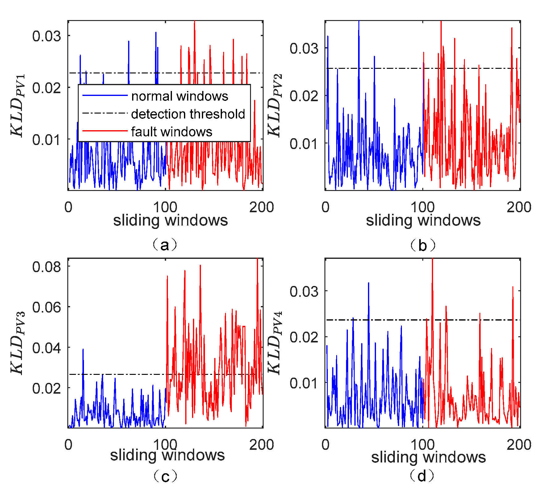
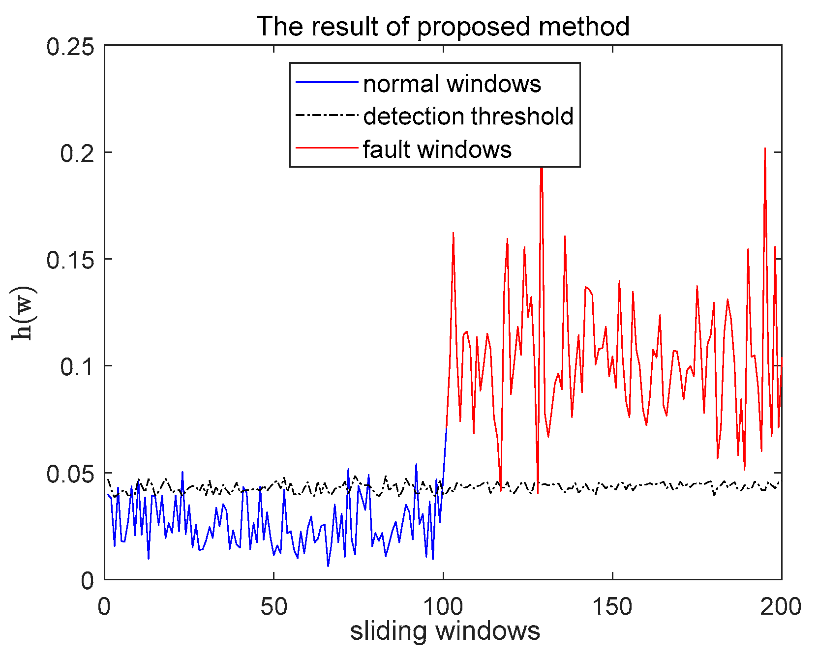
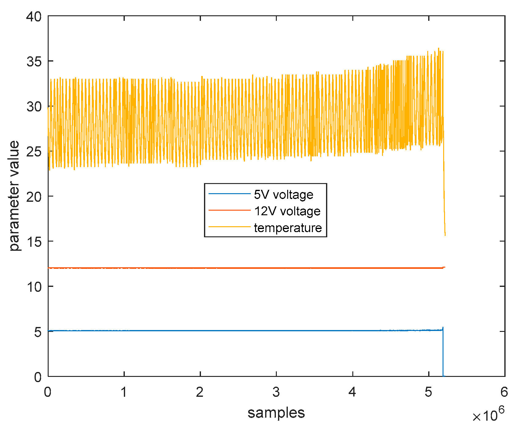
4.2. Satellite Spread-Spectrum Transponder Fault Case

4.2.1. The Phenomena and Causes of the Fault

On 3 October 2018, the downlink telemetry fault of a satellite spread spectrum transponder occurred. The ground telemetry, track and command (TT&C) station could not accept the satellite’s downlink telemetry signal, and the satellite telemetry remote communication returned to normal after enabling the backup spread spectrum transponder. After the incident, the data transmitted about the spread spectrum transponder telemetry showed that the spread spectrum transponder was in a shutdown state; the 5 V power telemetry jumped to 0 V; the solid-state amplifier current jumped from 0.715 A to 0.13 A; the solid-state amplifier power jumped from 11.19 w to 0.13 w; the temperature data showed the occurrence of the fault in the high-temperature region; the 12 V power telemetry slightly decreased; and other telemetry parameters were in the normal range. The spread spectrum transponder 5 V power telemetry performance before the jump to 0 is illustrated in Figure 10a. A similar exponential increase in the 5 V voltage before the fault and the eventual power failure is illustrated in Figure 10a.
The post-fault analysis located the fault as an anomaly in the DC–DC module of the spread spectrum transponder power module. This module is responsible for converting the voltage of the 42 V primary power supply to generate 5 V and 12 V power and then supplying power to the spread spectrum receiver and the spread spectrum transmitter. The analysis of the telemetry data of the occurrence of the fault shows that both the 5V and 12 V voltage fluctuations of the spread spectrum transponder are correlated with the temperature fluctuations of the spread spectrum transponder. As shown in Figure 10b, periodic fluctuations in the spread spectrum transponder temperature occurred because the satellite-Z surface where the stand-alone transmitter is located fluctuates periodically due to the influence of an external heat source. The 5 V voltage telemetry also fluctuated with the temperature before the fault. The 5 V voltage fluctuation to higher values mainly occurred in the high temperature region, while the 5 V voltage fluctuation to lower values mainly occurred in the low temperature region.

4.2.2. Results and Comparison of Detecting the Fault

We used a total of 5,215,000 samples of real telemetry data obtained from satellite measurements and control systems from 0:0:0 on 1 July 2018 to 8:05:49 on 3 October 2018. Each sample included three telemetry parameters: the spread-spectrum transponder temperature; the 5 V voltage of the spread-spectrum transponder; and the 12 V voltage of the spread-spectrum transponder, as shown in Figure 11. Due to the influence of the variation of satellite-Z’s angle to the sun, the temperature of the spread spectrum transponder drifts slowly with time. Consequently, in the experiment the temperature telemetry data were de-drifted. The sampling rate of all data was 1 Hz, and the satellite orbital period was 46,468 s. However, the data were discontinuous in time, which is due to the influence of the visible arc segment of the satellite and the ground station measurement and control resources. This resulted in telemetry data not being transmitted downward during part of the time.
In this article, the satellite orbital period was used as the length of the sliding window. The sliding window interval was 10,000 s, and a total of 539 sliding windows were retained with more than 20,000 samples within each sliding window. The first 380 sliding windows were selected as normal windows, and the last 159 sliding windows were used as on-line test windows. The first 64 windows in the on-line test windows were the normal windows, and the windows after that were the fault windows. The significance level of the PCA + KLD1 method and PCA + KLD2 method participating in the comparison were set to 0.05, 0.025 and 0.01, respectively, and significance level of the proposed method was set to 0.01.
Figure 12a–c shows the results of the spread spectrum transponder fault detection on the three PVs obtained from the PCA method. It can be seen from Figure 12 that only the second PV was sensitive to the fault. With a significance level of 0.01, there were still 23% of the fault windows located below the detection threshold. With a significance level of 0.025, 15% of the fault windows were still located below the detection threshold and a normal window was considered to be a fault window.
In comparison, Figure 13 shows the results of the proposed method for the spread-spectrum transponder fault. It is evident that the detection results on the local optimum PVs were better than those on the fixed PVs. Most of the fault windows were located above the detection threshold, with a high fault detection rate of 92.63% and a false alarm rate of 0%. With the significance level of 0.01, the PCA + KLD2 method can also obtain a 92.63% fault detection rate. However, 23.44% of the normal windows were considered to be fault windows. The fault detection results were calculated and are summarized in Table 2. This real case of detecting the fault in a satellite’s spread spectrum transponder further verifies the effectiveness and superiority of the method proposed in this paper.

5. Conclusions

The efficient detection and solving of incipient faults will effectively reduce the losses and the hazards they cause. Under the assumption that the variables obey a multidimensional Gaussian distribution, this paper models the optimum PV for detecting incipient faults as an optimization problem. Then, the validity of the proposed method is assessed using a numerical simulation example and an actual satellite fault case. Two different mitigation schemes are proposed to address the computational problem of the proposed method, in which the user can flexibly choose the sliding window interval or the alarm threshold according to the actual monitoring requirements and resource constraints. The method only has been proved in three faults. If the system was non-Gaussian or nonlinear, the detection effect of the proposed method might decrease. The future works related with improvement of the method can come from time efficiency and expansion to nonlinear systems. Although the proposed method is based on detecting incipient faults in satellites, it is not specific to this application of detecting faults in satellites and can be extended to other applications where multivariate statistical analysis can be used to detect incipient faults.

Author Contributions

Conceptualization, G.Z. and Q.Y.; software, G.Z.; validation, G.Z., Q.Y. and G.L.; formal analysis, G.Z.; investigation, G.Z.; resources, Q.Y. and J.L.; data curation, Q.Y. and J.L.; writing—original draft preparation, G.Z.; writing—review and editing, Q.Y., G.L. and L.W.; visualization, L.W.; supervision, G.L.; project administration, G.L.; funding acquisition, G.L. All authors have read and agreed to the published version of the manuscript.

Funding

This research was supported by Beidou Navigation In-orbit Support System, grant number JKBDZGDH01.

Institutional Review Board Statement

Not applicable.

Informed Consent Statement

Not applicable.

Data Availability Statement

Data available on request due to restrictions eg privacy or ethical. The data presented in this study are available on request from the corresponding author. The data are not publicly available due to privacy.

Conflicts of Interest

The authors declare no conflict of interest.

Abbreviations

FARfalse alarm rate
FDRfault detection rate
GPRGaussian Process Regression
IMSInductive Monitoring System
KLKullback–Leibler
KLDKL divergence
LOPVlocal optimum PV
LSTMLong Short-Term Memory
OS-SVMOne Class Support Vector Machine
PCAprincipal component analysis
PDFprobability density function
PVprojection vector

Mathematical Notations

SymbolSizeDescription
X n 0 × m Normal data matrix.
n 0 1 × 1 Number of normal samples
m 1 × 1 Number of variables of a system
X ¯ n 0 × m Normal data matrix after standardized.
Σ m × m Covariance matrix of X ¯
V m × m Eigenvector matrix of X ¯ , each column of the matrix V is a projection vector
n 1 1 × 1 Number of on-line samples
Y n 1 × m On-line data matrix.
v j m × 1 jth column of the matrix V
ε j 1 × 1 Detection threshold of the PV v j
α Significance level
μ x m × 1 Mean vector of the joint Gaussian distribution that the normal data obeyed
Σ x m × m Covariance matrix of the joint Gaussian distribution that the normal data obeyed
w m × 1 Optimum PV
μ y m × 1 Mean vector of the joint Gaussian distribution that the on-line data obeyed
Σ y m × m Covariance matrix of the joint Gaussian distribution that the on-line data obeyed
Δ μ m × 1 Mean deviation vector of μ x and μ y
h ( w ) 1 × 1 KL divergence of the projections of the normal data matrix X and the on-line data matrix Y on w
h X ( w ) r × 1 Vector of the KL divergences of the projections between all submatrices and the normal data matrix X on w
J ( w ) 1 × 1 Relative KL divergence of the projection of the normal data matrix X and the on-line data matrix Y on w
w 0 m × 1 Initial iteration vector
Y k n 1 × m On-line data extracted by the kth sliding window.
w k m × 1 Local optimum PV of the on-line data Y k and the normal data X
ε k 1 × 1 Detection threshold of the local optimal PV w k

References

  1. Jiang, H.; Zhang, K.; Wang, J.; Wang, X.; Huang, P. Anomaly Detection and Identification in Satellite Telemetry Data Based on Pseudo-Period. Appl. Sci. 2019, 10, 103. [Google Scholar] [CrossRef] [Green Version]
  2. Ezhilarasu, C.M.; Skaf, Z.; Jennions, I.K. The application of reasoning to aerospace Integrated Vehicle Health Management (IVHM): Challenges and opportunities. Prog. Aerosp. Sci. 2019, 105, 60–73. [Google Scholar] [CrossRef]
  3. Chandola, V.; Banerjee, A.; Kumar, V. Anomaly Detection: A Survey. ACM Comput. Surv. 2009, 41, 1–58. [Google Scholar] [CrossRef]
  4. Tipaldi, M.; Bruenjes, B. Survey on Fault Detection, Isolation, and Recovery Strategies in the Space Domain. J. Aerosp. Inf. Syst. 2015, 12, 235–256. [Google Scholar] [CrossRef]
  5. Youssef, A.; Delpha, C.; Diallo, D. Enhancement of incipient fault detection and estimation using the multivariate Kullback-Leibler Divergence. In Proceedings of the 2016 24th European Signal Processing Conference (EUSIPCO), Budapest, Hungary, 28 August–2 September 2016; pp. 1408–1412. [Google Scholar]
  6. Contreras-Reyes, J.E.; Arellano-Valle, R.B. Kullback-Leibler Divergence Measure for Multivariate Skew-Normal Distributions. Entropy 2012, 14, 1606–1626. [Google Scholar] [CrossRef] [Green Version]
  7. Chen, H.; Jiang, B.; Lu, N.; Mao, Z. Deep PCA Based Real-Time Incipient Fault Detection and Diagnosis Methodology for Electrical Drive in High-Speed Trains. IEEE Trans. Veh. Technol. 2018, 67, 4819–4830. [Google Scholar] [CrossRef]
  8. Narasimhan, S.; Brownston, L. HyDE—A General Framework for Stochastic and Hybrid Model-based Diagnosis. Proc. DX 2007, 7, 162–169. [Google Scholar]
  9. Deb, S.; Pattipati, K.R.; Shrestha, R. QSI’s Integrated Diagnostics Toolset. In Proceedings of the 1997 IEEE Autotestcon Proceedings AUTOTESTCON’97, Anaheim, CA, USA, 22–25 September 1997; pp. 408–421. [Google Scholar]
  10. Kurien, J.; R-Moreno, M.D. Costs and Benefits of Model-based Diagnosis. In Proceedings of the 2008 IEEE Aerospace Conference, Big Sky, MT, USA, 1–8 March 2008; pp. 1–14. [Google Scholar]
  11. Luo, B.; Wang, H.; Liu, H.; Li, B.; Peng, F. Early Fault Detection of Machine Tools Based on Deep Learning and Dynamic Identification. IEEE Trans. Ind. Electron. 2019, 66, 509–518. [Google Scholar] [CrossRef]
  12. Duncan Imbassahy, D.W.; Costa Marques, H.; Conceição Rocha, G.; Martinetti, A. Empowering Predictive Maintenance: A Hybrid Method to Diagnose Abnormal Situations. Appl. Sci. 2020, 10, 6929. [Google Scholar] [CrossRef]
  13. Pang, J.; Liu, D.; Peng, Y.; Peng, X. Optimize the Coverage Probability of Prediction Interval for Anomaly Detection of Sensor-Based Monitoring Series. Sensors 2018, 18, 967. [Google Scholar] [CrossRef] [Green Version]
  14. David, I.; Rodney, M.; Mark, S.; Spirkovska, L. General Purpose Data-Driven System Monitoring for Space Operations—AIAA Infotech@Aerospace Conference (AIAA). In Proceedings of the Aiaa Infotech, Seattle, WA, USA, 6–9 April 2009; pp. 26–44. [Google Scholar]
  15. Schwabacher, M.; Oza, N.; Matthews, B. Unsupervised Anomaly Detection for Liquid-Fueled Rocket Propulsion Health Monitoring. J. Aeros. Comp. Inf. Com. 2009, 6, 464–482. [Google Scholar] [CrossRef] [Green Version]
  16. Pang, J.; Liu, D.; Peng, Y.; Peng, X. Anomaly detection based on uncertainty fusion for univariate monitoring series. Measurement 2017, 95, 280–292. [Google Scholar] [CrossRef]
  17. Hundman, K.; Constantinou, V.; Laporte, C.; Colwell, I.; Soderstrom, T. Detecting Spacecraft Anomalies Using LSTMs and Nonparametric Dynamic Thresholding. In Proceedings of the 24th ACM SIGKDD International Conference on Knowledge Discovery & Data Mining, London, UK, 19–23 August 2018; pp. 387–395. [Google Scholar]
  18. Tariq, S.; Lee, S.; Shin, Y.; Lee, M.S.; Jung, O.; Chung, D.; Woo, S.S. Detecting Anomalies in Space using Multivariate Convolutional LSTM with Mixtures of Probabilistic PCA. In Proceedings of the 25th ACM SIGKDD International Conference on Knowledge Discovery & Data Mining, Anchorage, AK, USA, 4–8 August 2019; pp. 2123–2133. [Google Scholar]
  19. Yin, S.; Ding, S.X.; Xie, X.; Luo, H. A Review on Basic Data-Driven Approaches for Industrial Process Monitoring. IEEE Trans. Ind. Electron. 2014, 61, 6418–6428. [Google Scholar] [CrossRef]
  20. Li, X.; Zhang, X.; Zhang, P.; Zhu, G. Fault Data Detection of Traffic Detector Based on Wavelet Packet in the Residual Subspace Associated with PCA. Appl. Sci. 2019, 9, 3491. [Google Scholar] [CrossRef] [Green Version]
  21. Harmouche, J.; Delpha, C.; Diallo, D. Incipient fault detection and diagnosis based on Kullback-Leibler divergence using Principal Component Analysis: Part I. Signal Process. 2014, 94, 278–287. [Google Scholar] [CrossRef]
  22. Chen, H.; Jiang, B.; Lu, N. An improved incipient fault detection method based on Kullback-Leibler divergence. ISA Trans. 2018, 79, 127–136. [Google Scholar] [CrossRef]
  23. Youssef, A.; Delpha, C.; Diallo, D. An optimal fault detection threshold for early detection using Kullback-Leibler Divergence for unknown distribution data. Signal Process. 2016, 120, 266–279. [Google Scholar] [CrossRef]
  24. Song, B.; Zhou, X.; Tan, S.; Shi, H.; Zhao, B.; Wang, M. Process Monitoring via Key Principal Components and Local Information Based Weights. IEEE Access 2019, 7, 15357–15366. [Google Scholar] [CrossRef]
  25. Luo, L.; Bao, S.; Mao, J. Adaptive Selection of Latent Variables for Process Monitoring. Ind. Eng. Chem. Res. 2019, 58, 9075–9086. [Google Scholar] [CrossRef]
  26. Jolliffe, I.T. Principal Component Analysis, 2nd ed.; Springer: New York, NY, USA, 2002. [Google Scholar]
  27. Cherry, G.A.; Qin, S.J. Multiblock Principal Component Analysis Based on a Combined Index for Semiconductor Fault Detection and Diagnosis. IEEE Trans. Semicond. Manuf. 2006, 19, 159–172. [Google Scholar] [CrossRef]
  28. Doersch, C. Tutorial on Variational Autoencoders. arXiv 2016, arXiv:1606.05908. [Google Scholar]
  29. Huang, Y.; Zhang, Y.; Chambers, J.A. A Novel Kullback-Leibler Divergence Minimization-Based Adaptive Student’s t-Filter. IEEE Trans. Signal Process. 2019, 67, 5417–5432. [Google Scholar] [CrossRef]
  30. Kullback, S.; Leibler, R.A. On information and sufficiency. Ann. Math. Stat. Mar. 1951, 22, 79–86. [Google Scholar] [CrossRef]
  31. Byrd, R.H.; Gilbert, J.C.; Nocedal, J. A trust region method based on interior point techniques for nonlinear programming. Math. Program. 2000, 89, 149–185. [Google Scholar] [CrossRef] [Green Version]
  32. Coleman, T.F.; Li, Y. On the convergence of interior-reflective Newton methods for nonlinear minimization subject to bounds. Math. Program. 1994, 67, 189–224. [Google Scholar] [CrossRef]
  33. Nassar, B.; Hussein, W.; Mokhtar, M. Space Telemetry Anomaly Detection Based on Statistical PCA Algorithm. In Proceedings of the ICSSC 2015: International Conference on Satellite and Space Communications, Paris, France, 27–28 August 2015; pp. 637–645. [Google Scholar]
Figure 1. The process of obtaining vector h X ( w ) .
Applsci 11 00797 g001
Figure 2. The idea of hypothesis testing to detect incipient faults for each Y k .
Applsci 11 00797 g002
Figure 3. Results of detecting fault f 1 using the T 2 and squared prediction error (SPE) statistics: (a) T 2 statistic result for all on-line samples; (b) the result for the T 2 statistic at 1000 samples before and after insertion of the fault; (c) SPE statistic result for all on-line samples; (d) the result for the SPE statistic at 1000 samples before and after insertion of the fault.
Applsci 11 00797 g003
Figure 4. The results of detecting the incipient fault f 1 by using the principal component analysis (PCA) + Kullback-Leibler divergence (KLD)1 method and the PCA + KLD2 method: (a) the result of first projection vector (PV) for the fault f 1 ; (b) the result of second PV for the fault f 1 ; (c) the result of third PV for the fault f 1 ; (d) the result of fourth PV for the fault f 1 .
Applsci 11 00797 g004
Figure 5. The detection result of the proposed method for the incipient fault f 1 .
Applsci 11 00797 g005
Figure 6. The results of detecting the incipient fault f 2 by using the PCA + KLD1 method and the PCA + KLD2 method: (a) the result of first PV for the fault f 2 ; (b) the result of second PV for the fault f 2 ; (c) the result of third PV for the fault f 2 ; (d) the result of fourth PV for the fault f 2 .
Applsci 11 00797 g006
Figure 7. The detection result of the proposed method for the incipient fault f 2 .
Applsci 11 00797 g007
Figure 8. The results of detecting the incipient fault f 3 by using the PCA + KLD1 method and the PCA + KLD2 method: (a) the result of first PV for the fault f 3 ; (b) the result of second PV for the fault f 3 ; (c) the result of third PV for the fault f 3 ; (d) the result of fourth PV for the fault f 3 .
Applsci 11 00797 g008
Figure 9. The detection result of the proposed method for the incipient fault f 3 .
Applsci 11 00797 g009
Figure 10. The phenomena of the spread-spectrum transponder fault: (a) the spread spectrum transponder telemetry performance before failure; (b) the relationship of the 5 V voltage and the temperature.
Applsci 11 00797 g010
Figure 11. Raw telemetry data of the spread spectrum transponder.
Applsci 11 00797 g011
Figure 12. The results of detecting the spread-spectrum transponder fault by using the PCA + KLD1 method and the PCA + KLD2 method at different significance levels: (a) the result of first PV for the fault; (b) the result of second PV for the fault; (c) the result of third PV for the fault.
Applsci 11 00797 g012
Figure 13. The detection result of the proposed method for the spread-spectrum transponder fault.
Applsci 11 00797 g013
Table 1. Comparison of the performance of five different methods at detecting the three faults.
Faults PCA + T 2 PCA + SPEPCA + KLD1PCA + KLD2Proposed Method
FDRFARFDRFARFDRFARFDRFARFDRFAR
f 1 1.09%1.01%1.20%1.01%79.63%4.87%98.04%9.50%98.11%8.10%
f 2 1.45%0.98%2.13%1.02%13.83%4.63%62.92%9.01%84.77%7.48%
f 3 1.04%0.99%1.02%1.01%4.38%3.70%35.17%9.20%98.33%8.05%
Average value1.19%1.00%1.45%1.01%32.61%4.73%65.38%9.24%93.74%7.88%
Table 2. Comparison of the performance of three different methods at detecting the spread-spectrum transponder fault.
MethodsPCA + KLD1PCA + KLD2Proposed Method
Significance Level0.050.0250.010.050.0250.010.01
FDR76.84%84.21%92.63%76.84%84.21%92.63%92.63%
FAR0%3.13%23.44%0%3.13%23.44%0%
Publisher’s Note: MDPI stays neutral with regard to jurisdictional claims in published maps and institutional affiliations.

