Article

Innovatively Fused Deep Learning with Limited Noisy Data for Evaluating Translations from Poor into Rich Morphology

by
Despoina Mouratidis
1,*,
Katia Lida Kermanidis
1 and
Vilelmini Sosoni
2
1
Department of Informatics, Ionian University, 491 00 Corfu, Greece
2
Department of Foreign Languages, Translation and Interpreting, Ionian University, 491 00 Corfu, Greece
*
Author to whom correspondence should be addressed.
Appl. Sci. 2021, 11(2), 639; https://doi.org/10.3390/app11020639
Submission received: 18 December 2020 / Revised: 1 January 2021 / Accepted: 4 January 2021 / Published: 11 January 2021
(This article belongs to the Special Issue Machine Learning Methods with Noisy, Incomplete or Small Datasets)

Abstract

:
Evaluation of machine translation (MT) into morphologically rich languages has not been well studied despite its importance. This paper proposes a classifier, that is, a deep learning (DL) schema for MT evaluation, based on different categories of information (linguistic features, natural language processing (NLP) metrics and embeddings), by using a model for machine learning based on noisy and small datasets. The linguistic features are string based for the language pairs English (EN)–Greek (EL) and EN–Italian (IT). The paper also explores the linguistic differences that affect evaluation accuracy between different kinds of corpora. A comparative study between using a simple embedding layer (mathematically calculated) and pre-trained embeddings is conducted. Moreover, an analysis of the impact of feature selection and dimensionality reduction on classification accuracy has been conducted. Results show that using a neural network (NN) model with different input representations produces results that clearly outperform the state-of-the-art for MT evaluation for EN–EL and EN–IT, by an increase of almost 0.40 points in correlation with human judgments on pairwise MT evaluation. It is observed that the proposed algorithm achieved better results on noisy and small datasets. In addition, for a more integrated analysis of the accuracy results, a qualitative linguistic analysis has been carried out in order to address complex linguistic phenomena.

1. Introduction

Machine translation (MT) applications have nowadays infiltrated almost every aspect of everyday activities. For the development of efficient MT solutions, reliable automated evaluation schemata are required. Over the past few years, neural network (NN) models have improved the state-of-the-art of different natural language processing (NLP) applications [1], such as language modeling [2,3], improving answer ranking in community question answering [4], improving translation modeling [5,6,7], as well as evaluating machine translation output [4,8,9]. Embeddings are a powerful way of representing text, provided that they are able to capture the linguistic identity (morphosyntactic and semantic profile) of a sentence/word. In 2013, Mikolov et al. [3] released the word2vec library. Word2vec became quickly the dominant approach for vectorizing textual data. The NLP models that were already well studied based on traditional approaches, such as latent semantic indexing (LSI) and vector representations using term frequency–inverse document frequency (TF-IDF) weighting, have been tested against word embeddings and, in most cases, word embeddings have come out on top. Since then, the research focus has shifted towards embedding approaches.
The present study aims to find out how embeddings, obtained through various means, in combination with different kinds of information fuse, affect classification accuracy small and noisy dataset, when used to train a model to choose the best translation output. The target languages (in contrast to the source language) are rich in morphology, as the proposed schema is applied to the English–Greek (EN–EL) and English–Italian (EN–IT) language pairs. Greek and Italian languages have a rich inflectional morphology, as the nouns have different grammatical morphemes for the genders and the verbs have different grammatical morphemes for the two numbers and for the first, second and third person as well. In particular, the proposed NN learning schema is set up to test:
  • two different forms of text structure (an informal (noisy) corpus (C1), and a formal, well-structured corpus (C2)) will be experimented with;
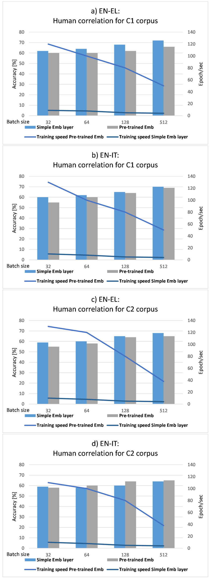
  • a comparative analysis of two different ways of calculating embeddings (the straightforwardly mathematically calculated layer embeddings and the use of pre-trained embeddings) will be conducted
  • the application of the SMOTE [10] oversampling technique during training will be investigated in order to overcome data imbalance phenomena;
  • the use of two string-based linguistic features (hand-crafted), that capture the similarity between the MT outputs and the reference translation (Sr).
Further innovative aspects of the present work include:
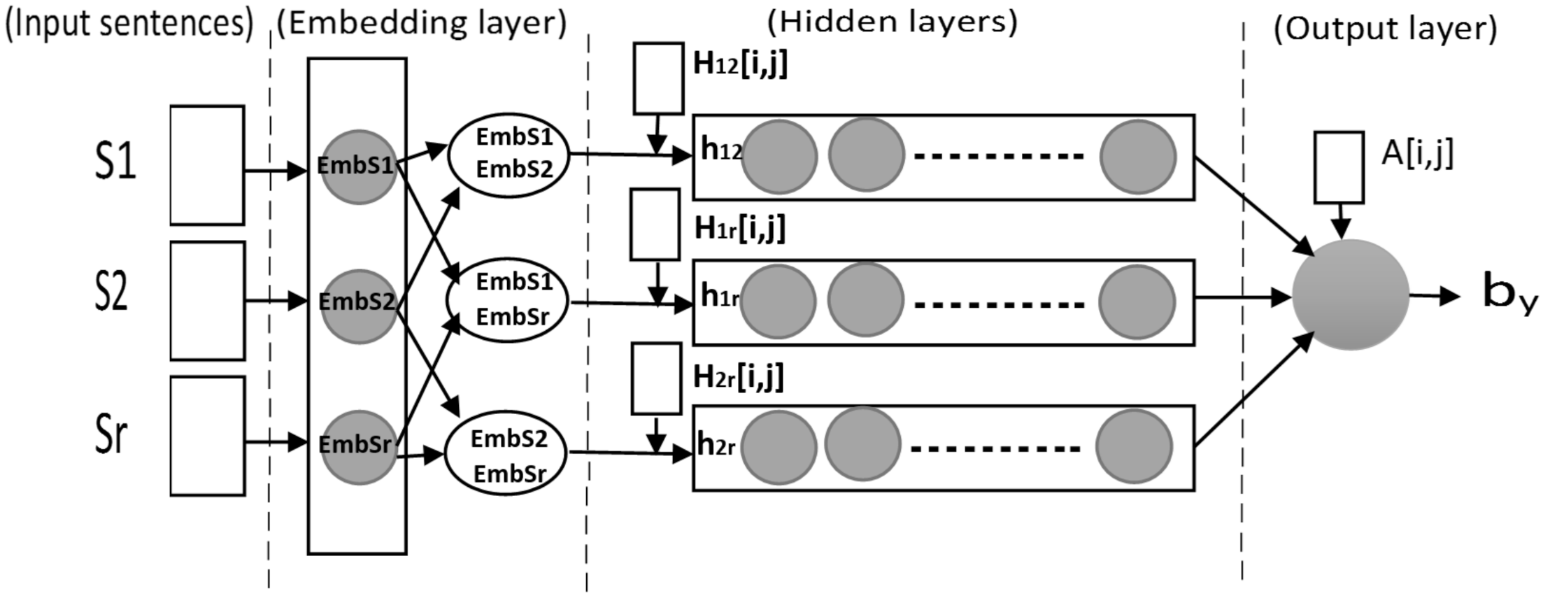
  • a novel deep learning architecture with innovative feeding structure that involves features of various linguistic levels and sources;
  • a qualitative linguistic analysis that aims to reveal linguistic phenomena linked to poor/rich morphology, that impact on translation performance;
  • the exploration of two different validation options (k-fold cross validation (CV) and Percentage split);
  • the application of feature selection and dimensionality reduction methods;
  • the application of the proposed multi-input, multi-level learning schema on text data from very different genres.
The rest of the paper is organized as follows—Section 2 presents the related work in the addressed scientific area. Section 3 describes the data sets (corpora), the feature set used, the learning framework and the network settings. Section 4 describes more experimental details and the results of the classification process. Finally, Section 5 presents the paper’s conclusions and directions for future research.

2. Related Work

Some of the most popular methods in automatic MT evaluation rely on score based metrics. These metrics include (i) metrics based on n-gram counts, such as Bilingual Evaluation Understudy (BLEU) [11] and National Institute of Standards and Technology (NIST) [12], or on the edit distance, like Word Error Rate (WER) [13], (ii) metrics using external resources, like WordNet and paraphrase databases—METEOR [14] and Translation Error Rate (TER) [15], (iii) metrics based on lexical similarity or syntactic similarity (involving higher level information, such as part of speech tags (POS)) between the MT outputs and the reference, and iv) neural metrics such as ReVal [8] and Regressor Using Sentence Embeddings (RUSE) [16], which directly learn embeddings for the entire translation and reference sentences using long short-term memory (LSTM) networks and pre-trained sentence representations.
Several research approaches on text classification, system ranking and selection techniques have been proposed using machine learning schemata. Guzmán et al. [4] focus on a ranking approach based on predicting BLEU scores. Duh [17] decomposes rankings into parallel decisions, with the best translation for each candidate pair predicted, using a ranking-specific feature set and BLEU score information. The framework involves a Support Vector Machine (SVM) classifier. A similar pairwise ranking approach was proposed by Mouratidis and Kermanidis [9], using a random forest (RF) classifier.
Neural networks are also used in the literature frameworks. Recurrent neural networks (RNN) and long short term memory (LSTM) networks [18], which are widely popular for learning sentence representations, have been taken up widely in a variety of NLP tasks [6,7]. Cho et al. [7] proposed a score-based scheme to learn the translation probability of a source phrase to a target phrase (MT output) with an RNN encoder-decoder. They showed that this learning scheme has improved the translation performance. The scheme proposed by Sutskever et al. [19] is similar to Cho et al. [7] work, but Sutskever et al. [19] chose the top 1000 best candidate translations produced by a Statistical Machine Translation (SMT) system with a 4-layer LSTM sequence-to-sequence model. LSTM networks are also widely adopted in MT evaluation [8]. LSTM memory units incorporate gates to control the information flow and they can preserve information for long periods of time. Wu et al. [20] trained a deep LSTM network to optimize BLEU scores when translating from English to German and English to French, but they found that the improvement in BLEU scores did not reflect the human evaluation of translation quality. Mouratidis et al. [21] used LSTM layers in a learning framework for evaluating pairwise MT outputs using vector representations, in order to show that the linguistic features of the source text can affect MT evaluation. Convolutional neural networks (CNN) are less common for sequence to sequence modeling, despite several advantages [22]. Compared to RNN, CNN create representations for fixed size contexts and do not depend on the computations of the previous time step because they do not maintain a hidden state. Gehring et al. [23] proposed an architecture for sequence to sequence modeling based on CNN. The model is equipped with linear units [24] and residual connections [25]. They also used attention in every decoder layer and demonstrated that each attention layer only adds a very small amount of overhead. Vaswani et al. [26] proposed a self-attention-based model and dispensed convolutions and recurrences entirely. Bradbury et al. [27] introduced recurrent pooling between a succession of convolutional layers, while Kalchbrenner et al. [28] studied neural translation without attention.
However, little attention has been paid to their direct applicability to languages with rich morphology. The present work focuses on the automatic evaluation of translation into morphologically rich languages, (Greek and Italian). The aim of this work is to identify the input information that is more effective for feeding a learning schema. Input information is investigated according to certain criteria, that is, the different means of calculating embeddings, the features of varying levels of linguistic information, the different dataset genres.

3. Materials and Methods

This section describes the dataset, the linguistic features and the NN architecture used in the experiments.

3.1. Dataset

In these experiments, two different types of parallel corpora in the two language pairs (EN-EL and EN-IT) are used. The first dataset (C1) consists of the test sets developed in the TraMOOC project [29]. It is a small and noisy dataset as it is comprised of educational video lecture subtitles, lecture presentation slides and assignments, while it contains mathematical expressions, spoken language features, fillers, repetitions, and many special characters, such as /, @. The second formal dataset (C2) consists of parallel corpora from European Union legal documents, found on EUR-Lex, the online gateway to European Union Law, under the category “Consolidated texts”. The chosen sentences are from Directives, Decisions, Implementing Decisions, Regulations and Implementing Regulations of the European Council and the European Commission, on the following issues: general, financial and institutional matters, competition and development policy, energy, agriculture, economic, monetary and commercial policy, taxation, social policy and transport policy. As pointed out, C1, is not a well-structured corpus as it contains linguistic phenomena which are unorthodox and ungrammatical, like misspellings, repetitions, fillers, disfluencies, spoken language features and so forth. On the other hand, C2 is formal language text. For the C1 corpus it was necessary to perform data pre-processing, that is, removal of special symbols (@, /), and alignment corrections. For the C2 corpus no pre-processing was required. Two MT outputs were used - one generated by SMT models, that is, the Moses toolkit [30] for C1 and Google Translate [31] for C2, and the second was generated by Neural Machine Translation (NMT) models, that is, the Nematus toolkit [32] for C1 and Google Translate for C2. The Moses and Nematus prototypes are trained in both in- and out- of domain data. The Nematus is trained on additional in-domain data provided via crowdsourcing, and also includes layer normalization and improved domain adaptation. In-domain data included data from TED, Coursera, and so forth [33]. Out-of-domain data included data from Europal, OPUS, WMT News corpora and so forth. The Google Translate prototype was trained on over 25 billion examples. More details about the corpora are presented in Table 1.

3.2. Features

The employed feature set is divided into two categories: one consisting of hand-crafted string-based features from the MT outputs, SSE and Sr, and the other consisting of commonly used NLP Metrics. The first category contains (i) simple features (e.g., distances like Levenshtein [34], longest word for S1, S2, Sr, SSE, features using the Length Factor (LF) [35]), (ii) features identifying the noise in the corpus (e.g., repeated words/characters, unusually long words in number of characters), and (iii) features providing linguistic information from the SSE in EN (e.g., the length of the SSE in number of words and number of characters). The feature set was inspired by the work of References [36,37]. The second category contains the NLP metrics, that is, the BLEU score, METEOR, TER and WER for (S1, S2), (S1, Sr), (S2, Sr). To calculate the BLEU score, an implementation of the BLEU score from the Python Natural Language Toolkit library [38] is adopted. For the calculation of the other three metrics, the code from GitHub [39] is used. The total number of features is 82. A detailed description of the feature set can be found in Reference [21].
In the present work, the employed feature set is extended and two additional novel linguistic feature pairs, which belong to the first category, have been used (increasing thereby the feature dimensions from 82 to 86). These features are similarity-based. The first feature cmt shows the percentage of identical words between the MT outputs and Sr, without taking into account the word order. The second feature rmt shows the percentage of identical parts of MT output included in the Sr. More specifically, this feature shows whether the MT output is a contiguous subsequence of Sr. The features are defined in Equations (1) and (2) respectively:
c m t = | S m t S r | | S m t S r |
r m t = | S m t S r | | ( S m t S r ) | with | ( S m t S r ) | 0 .
where Smt is one of the S1, S2.
As an example, if
Sr = {η (the), υπηρεσία (department), προσδιορίζει (specify), το (the), διάστημα (period)},
S1 = {το (the), χρονικό (time), διάστημα (period), η (the), υπηρεσία (department), καθορίζει (determines)},
S2 = {η (the), υπηρεσία (department), προσδιορίζει (specify), την (the), περίοδο (period)}, then cmt = 0.57, rmt = 1.3 for S1 MT output and cmt = 0.43, rmt = 0.75 for S2 MT output.
All feature values were calculated using MATLAB, and their values have been normalized and vary between 0 and 1.

3.3. Embedding Layers

Firstly, an embedding layer (mathematically-calculated embeddings) is used for the two MT outputs and the Sr. The encoding function applied is the one-hot function. The embedding layer size, in number of nodes, is 16. The input dimensions of the embedding layer is in agreement with the vocabulary of each language, taking into account the most frequent words (500 for EN-EL/700 for EN-IT). The embedding layer used is the one provided by Keras [40]. Secondly, a Greek version of WordSim353 [41] is adopted for pre-trained embeddings. More specifically WordSim353 contains the 300-dimensional Greek embeddings of 350 K words, trained on 20 M of URLs with Greek language content and they computed in 2018. More details about the number of unique sentences, unigrams, bigrams, trigrams and so forth can be found in Outsios et al. [41]. In this case, the embedding layer utilized the embedding matrix produced by the embedding_index dictionary and the word_index. The Embedding layer should be fed with padded sequences of integers. For this purpose, the keras.preprocessing.text.Tokenizer and the keras.preprocessing.sequence.pad_sequences [40] were run. For the pre-trained Italian embeddings, the Wikipedia2Vec tool is used [42]. The size, in number of nodes, of the embedding layer is 300, as is the dimension of pre-trained embeddings for both datasets.

3.4. NN Architecture

This study aims to identify the best MT output out of the two provided. Two linguists annotated the sentences with 1 if the NMT output is better than the SMT one and with 0 if the SMT output is better than the NMT. A low annotation percentage is observed for the SMT class (EL: 37% for C1, 48% for C2, IT: 43% for C1, 48% for C2) compared with the NMT class (EL: 63% for C1, 52% for C2, IT: 57% for C1, 52% for C2). A low annotation agreement rate is observed (C1: 5% for EN-EL/6% for EN-IT, C2: 3% for EN-EL/5% for EN-IT). For the few different answers, the annotators had a discussion and finally agreed on one common label. The NN model takes as input the tuple (S1, S2, Sr). These sentences are passed to the embedding layer. Two ways for extracting embeddings are applied (described in Section 3.3) producing EmbS1, EmbS2, EmbSr. The EmbS1, EmbS2, EmbSr vectors are concatenated in a pairwise fashion as (EmbS1, EmbS2), (EmbS1, EmbSr), (EmbS2, EmbSr), and they form the input to the similarity-based hidden layers h12, h1r, h2r. As extra inputs, the hidden layers are fed with the matrices H12[i,j], H1r[i,j], H2r[i,j] (where i is the number of sentences and j the number of features), containing the second category features (NLP set). The hidden layer outputs form the input to the output layer. Moreover, an extra input to the output layer is used: the matrixA[i,j], containing the first category features (described in Section 3.2). The DL NN schema is shown in Figure 1.
The binary classification problem is modeled as a Bernoulli distribution (Equation (3)):
Y B e r n o u l l i ( Y b y ) ,
where by is the sigmoid function σ ( w T x + b ) , w T and b are the network’s parameters.

3.5. Network Settings

The network model architecture for the experiments is a classic architecture of RNN networks (2 LSTM layers with 400 hidden units) and feedforward layers (4 Dense layers, that is, 3 layers with 50 hidden units and 1 layer with 400 hidden units). The network is trained using the Adam optimizer [43] to optimize parameters. To avoid over-fitting, dropout is applied with a rate of 0.05, using the loss function of binary cross entropy and the regularization parameter λ is set equal to “ 10 3 ”. 10-fold CV and 70% percentage split were employed for testing.

4. Results

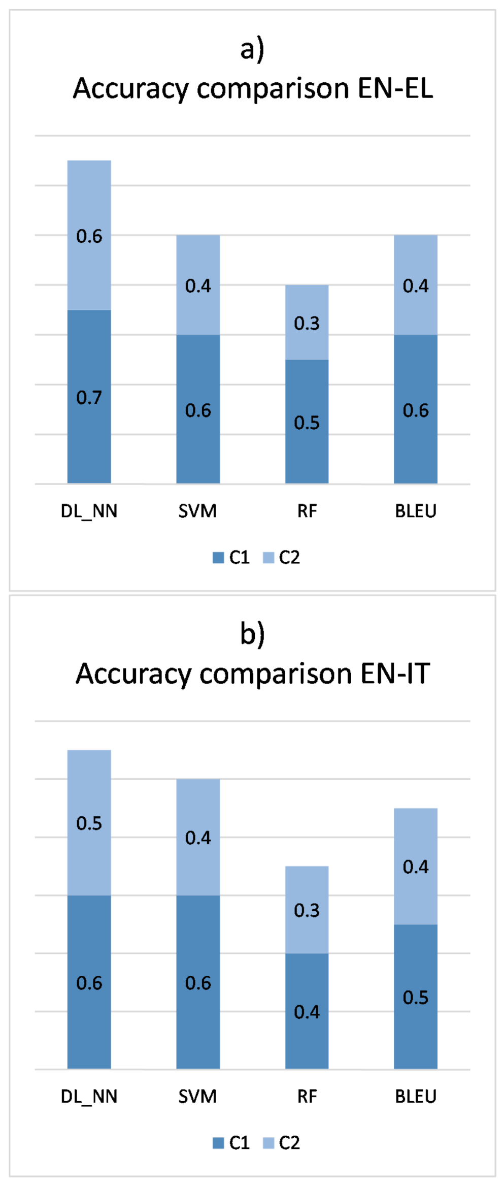
4.1. Performance Evaluation

In this experiment (a) we investigate whether the predicted classifications have any correlation with human annotation, (b) we compare the proposed classification mechanism against the baseline classification models for small noisy and formal datasets respectively, (c) we compare two different ways of generating the embedding layer, and (d) we test two different options of validation methods. Table 2 presents the classification results (Precision and Recall) for the different MT outputs over the two different datasets. The C1 corpus presents a classification increase, for both language pairs (accuracy: 72% EN-EL/70% for EN-IT), in contrast to the C2 corpus (accuracy: 68% for EN-EL/65% for EN-IT), even though the C1 corpus contains a lot of noise. This is probably due to the fact that the C1 corpus contains more sentences, and, also, because the C2 corpus has richer vocabulary and more formal structure. It is more difficult for the classifier to choose the best MT output, because the SMT output is more similar to the NMT output in this corpus (C2). It is also observed that both evaluation metrics chose the NMT model over the SMT one, which is in accordance to the annotators’ results. In addition, the aforementioned accuracy results are obtained when the NN uses the simple embedding layer. However, when the pre-trained embeddings are used, the model does not lead to better results (average accuracy of C1 and C2: 66% for EN-EL/65% for EN-IT), since the embeddings are trained on the general-purpose corpus, which is not representative of the input corpora used therein. At this point, it is worth mentioning that the pre-trained embeddings seem to be more effective for the EN-IT pair than for the EN-EL language pair. As far as the different types of corpora are concerned, pre-trained embeddings are more efficient for the C2 corpus (average accuracy of EN-EL and EN-IT: 66%) than the C1 corpus (average accuracy of EN-EL and EN-IT: 64%). This is probably due to the fact that the C2 corpus has richer vocabulary than the C1 corpus.
An approach to improve the classification accuracy of a small and noisy dataset is to apply the SMOTE oversampling technique on the training data. Using SMOTE, the sentences of the minority class (SMT) doubled in number, and the total number of sentences reached 3024 for C1 and 2276 for C2. It is important to compare the performance between the 82 and the 86 feature dimensions, with and without the SMOTE filter. When SMOTE is applied, a small accuracy increase is observed on the 82 features (average accuracy of C1 and C2: 68% for EN-EL/67% For EN-IT), and an even higher increase on the 86 features (average accuracy of C1 and C2: 70% for EN-EL/68% for EN-IT). It is interesting that the EN-EL corpora outperformed EN-IT in all the experiments. The results with the use of the two new suggested features are generally better for both corpora and language pairs.
Firstly, k-fold CV was used, which is a reliable method for testing the models, and a value of k = 10 is very common in the field of machine learning [44] (Table 2). Secondly, part of the data (70%) is kept for training, and part (30%) is applied for testing (Table 3). Given that both classes are of interest, the symmetric Matthews correlation coefficient (MCC) metric [45] (a special case of the ϕ phi coefficient [46]) is used, as it constitutes a good way to describe the relation of TP (true positive), FP (false positive) and FN (false negative) values by a single number. It is defined as follows:
M C C = T P × T N + F P × F N ( T P + F P ) × ( T P + F N ) × ( T N + F P ) × ( T N + F N ) .
When using 10-fold CV, C1 outperforms C2 for both language pairs. When the percentage split method (70% training–30% testing) is used, a small performance improvement is observed for the C2 corpus. Moreover, MCC achieves higher value for the C2 corpus, when pre-trained embeddings are used.
Figure 2 shows the accuracy performance according to training speed and batch size. Increasing the batch size can increase the model’s accuracy. As seen above, the training speed decays more quickly for the simple embedding layer compared to the pre-trained embedding layer model. Moreover, the accuracy of the pre-trained embeddings is consistently higher for corpus C2. The best performance has been consistently obtained for batch size 512.
It is important to analyze the correlation with human-performed evaluations [47]. In this work, the correlation of the predicted scores with human judgments is reported using Kendal τ . Kendall τ , is a coefficient that measures the agreement between rankings produced by human judgments, and rankings produced by the classifier. The WMT’12 (Workshop of Machine Translation) definition of Kendall’s τ is used, and it is calculated as follows:
τ = ( c o n c o r d a n t p a i r s d i s c o r d a n t p a i r s ) t o t a l p a i r s
where ‘concordant pairs’ is the number of times the human judgment and the predicted judgment agree in the ranking of any two translations that belong to the same SSE, and ‘discordant pairs’ is the opposite.

4.1.1. Comparison to Related Work

As mentioned earlier, there is limited work on pairwise evaluation based on the small and noisy dataset. In order to compare our results with other methods, additional experiments were reproduced in order to imitate as closely as possible earlier work settings, that were (i) based on different classifiers such as SVM [17] and RF [37] and (ii) based on other evaluation methods, that is, the use of the BLEU score [4,17].
Figure 3 shows the overall Kendall τ for the different approaches. The proposed DL schema has achieved comparable performance to the models proposed in earlier works. The SVM classifier succeeds in a strong positive relationship between the two classes for C1_EN-EL: 0.7, and moderate positive relationship for C2_EN-EL: 0.4, C1_EN-IT: 0.4 and C2_EN-IT: 0.6, while the RF classifier reached a moderate positive relationship for the C1 corpus (0.4 for EN-EL/0.6 for EN-IT) and for the C2 corpus (0.4 for EN-EL/0.6 for EN-IT). When the BLEU score information is used, the model achieved a moderate positive relationship. Kendall τ reached its highest value when the proposed schema uses the simple embedding layer, the feature set of 86 dimensions, and the NLP set for both language pairs (EN-EL: 0.7 for C1/0.6 for C2 and EN-IT: 0.6 for C1/0.5 for C2).

4.1.2. Feature Selection and Dimensionality Reduction

There are many techniques for improving the classifier’s performance. Feature selection (FS) and Dimensionality reduction (DR) are two commonly used techniques that improve classification accuracy [48]. The main idea behind FS is to remove redundant or irrelevant features that are not useful for the classifier [49]. The advantage of FS is that no information about the importance of single features is lost. With DR the size of the feature space is decreased, but without losing vital information [50].
FS methods are usually categorized in two basic methods: wrappers and filters [51]. Wrapper FS methods evaluate multiple models with different subsets of input features and select those features that result in the best performing model according to a performance metric. The number of possible results will increase geometrically as the number of features increases. Filter FS methods use statistical techniques to evaluate the relationship between each input variable and the target variable, and these scores are used as the basis to choose (filter) those input variables that will be used in the model. Filters are either global or local. Global methods assign a single score to a feature regardless of the number of classes while local methods assign several scores, as every feature in every class has a score [52]. Global methods typically calculate the score for every feature and then choose the top-N features as the feature set, where N is usually determined empirically. Local methods are similar but require converting a feature’s single score before choosing the top-N features. Wrappers require much more computation time than filters, and may work only with a specific classifier [51].Filters are the most common FS method for text classification. Some commonly used FS methods are a. Recursive Feature Elimination Cross Validation (RFECV) that belongs to the Wrappers methods, b. the information gain (IG) [53] that belongs to filter global FS methods, and c. the Chi-square (CHI) [54], that belongs to the filter local methods. All these FS methods are language-independent feature selection methods that produce better accuracy.
In these experiments RFECV is tested using Support Vector Machines (SVM) with linear kernel and the number of cross validation folds is set to 10. Information gain is often applied to find out how well each single feature A separates the given feature data set S and it is calculated as follows:
I G ( S , A ) = I ( S ) n A = | S n | | S | I ( S n ) ,
where n is the value of every feature (A) and S v is the set of instances where A has value n.
CHI is a supervised FS method that calculates the correlation of a feature value n with the class m, and it calculated as follows:
x 2 = i = 1 n i j = 1 m j = ( O i j E i j ) 2 E i j ,
where O i j is the observed frequency and E i j is the expected frequency.
DR refers to algorithms and techniques that create new features which are combinations of the old features [54]. The most important DR technique is principal component analysis (PCA) [55]. PCA is an unsupervised dimensional reduction technique. PCA produces new features from the original features by converting the high dimensional space of the original features to a low dimensional space while keeping linear structure. Dimensionality reduction is accomplished by choosing enough eigenvectors to account for some percentage of the variance in the original data (a default value is 0.95). Attribute noise was filtered by transforming the original into the PC space, eliminating some of the worst eigenvectors, and then transforming back to the original space. The maximum number of attributes to include in the transformed space was set to 5.
Better accuracy results are observed, in general, when a feature selection method is used, in contrast to the whole feature set model (Table 4). The accuracy performance increased 4% for the C1 corpus for EN-EL and 3% for EN-IT. It seems that the application of these methods is more efficient for the SMT for the informal C1 corpus and NMT for the formal (well-structured) C2 corpus. More specifically, there is an increase up to 4% for the SMT class for C1 and 2% for C2, while, for the NMT class, there is 2% for C1 and C2. In addition, the feature selection methods work better for C1 (an increase up to 3.5% in average for both language pairs) rather than the C2 (an increase up to 2.5% in average for both language pairs). We conclude that feature selection methods help more the noisy corpus. This is in accordance with the accuracy results of the previous model.
Concerning the features, it is verified that, for the proposed model, the more effective features are those containing ratios, features identifying the presence of noise in a segment (for example the occurrence of repeated characters) and features used linguistic information from the SSE. They all seem to be useful for prediction. Also, the new string-based features added in this paper are presumed to enclose valuable information for the model as they capture the similarity between the MT outputs and the reference translation. The new string-based features were selected almost from every method. Regarding the FS method, it seems that better accuracy results were produced with CHI square and IG. Additionally, it is observed that the feature reduction space method (PCA) does not help the accuracy performance regardless of the corpora structure-type, since in all experiments the performance was less than or equal to the classifier performance using the whole feature set.

4.2. Linguistic Analysis

In order to have a more comprehensive analysis of the accuracy results, we have carried out a qualitative linguistic analysis as well. In this context, problems have been identified regarding some complex linguistic phenomena for both language pairs (Table 5).
For the first sentence (ID1): (Both NN and the Annotator’s choice was S2)
  • The verb to deploy means: to develop, to emplace, to set up. Both S1 and S2 erroneously translated that verb as to use. Nevertheless, the verb to use is one of the secondary meanings of the verb to deploy.
  • The most common meaning of the word bug is insect, virus, but it also means: error. The word fix means repair, determine, nominate. In this sentence, bug fix is used as a noun phrase, where the first word functions as a subjective genitive, and the phrase means: error correction. S1 commits two errors when translating “fix” (φτιάξουμε), i. Fix is erroneously considered to have a verb function. ii. It is difficult to explain why the same verb is translated in the first person of plural of the simple past-subjunctive. As a consequence, S1, S2’s translations for the verbal phrase (deploys a bug fix) are both nonsensical: S1: “χρησιμοποιεί ένα έντομο φτιάξουμε” (“uses an insect” + simple past-subjunctive of “repair”), S2: χρησιμοποιεί “ένα σφάλμα για τα έντομα” (uses an error for the insects).
  • In addition, it is important to notice that S2 has translated the same phrase (bug fix) at the end of the sentence in a different way. S2 tried to improve the translation and it certainly succeeded, but only for the word fix (διόρθωση). S2 also “spotted” that bug is a subjective genitive (the correction of the error), but it still identified bug as an insect and it has erroneously translated it: ζουζιού. In Greek, this is a nonexistent word, but it is strongly reminiscent of the word ζουζούνι (insect), which is an onomatopoeic word (the buzz of a bug) and especially of its genitive case: ζουζουνιού, with some letters missing.
  • S1 has correctly “identified” the meaning of the verb to list (to enumerate), but not in the correct grammatical number—third-person plural, instead of third-person singular. S2 chose the correct grammatical inflectional morphemes for the number and the person, but not the correct meaning, for this context: referred, instead of enumerated, indexed or set out. So, the proposed NN model has correctly chosen S2, as S2 “recognized” the correct grammatical morphemes of number and person features.
  • Regarding the passive future verb: will be updated: In S1, the preceding particle of future tense in Greek θα (According to the Cambridge Dictionary, a particle is a word or a part of a word that has a grammatical purpose but often has little or no meaning. https://dictionary.cambridge.org/dictionary/english/particle) (will) is separated from the subjunctive (επικαιροποιηθεί), which is wrong.
  • Both S1 and S2 have erroneously translated the noun phrase: cache manifest. As they failed to identify the multi-word expression, they have translated them separately. The word cache means: crypt, hideout, cache memory, and, in this sentence, it has the last meaning (κρυφή μνήμη). However, S1 “chose” the first meaning (κρύπτη) (crypt), whereas S2 left the word untranslated. Manifest means obvious, apparent. Both S1 and S2 “chose” from these synonyms. Nevertheless, the cache manifest in HTML5 is a software storage feature which provides the ability to access a web application even without a network connection (https://en.wikipedia.org/wiki/Cache_manifest_in_HTML5). So, the best translation would be: κρυφή μνήμη ιστότοπου (website cache memory), a translation that was not even produced in the reference.
For the second sentence (ID2): (NN chose S1/Annotator’s choice was S2)
  • Sit: Both S1 and S2 have erroneously translated this verb (κάτσετε, καθήσετε). In this sentence, the verb to sit is transitive and means: to place, to put, requiring an inanimate object, whereas the very common meaning of this verb, that is to have a seat, presupposes that the verb is intransitive (+animate subject) or transitive (but:+animate object: I make someone sit down). Both S1 and S2 have erroneously adopted the second meaning, without “noticing” that its object (spheroids) is an inanimate noun. Even more, the form chosen by S1 belongs to oral speech (κάτσετε) (to sit), while S2’s form is misspelled (καθήσετε (to sit), instead of the correct: καθίσετε).
  • Kind of is an informal expression modifying and especially attenuating (It is the opposite of really. In the UK, it is considered quite informal. https://english.stackexchange.com/questions/296634/kind-of-like-is-a-verb) the meaning of the verb plonk. S1 has erroneously “identified” that word as a noun and so mistranslated it as: form, genre, species(είδους). Nevertheless, S1 “identified” the inflectional grammatical morpheme of the genitive case:-ους for of.
  • Plonk down: This phrasal verb has a lot of meanings: drop heavily, place down, impale, attract and so forth (https://glosbe.com/en/el/plonk%20down) S1 has erroneously translated this verb in the meaning of impale, which is not the case. S1 has separately translated the whole sentence (they kind of plonk down: είδους παλουκώσει τους κάτω), which is completely nonsensical in Greek. In addition, the verb object them has been erroneously placed after the verb (in Greek, the clitic form of the personal pronoun is placed before the verb) and has been translated by a wrong grammatical morpheme (masculine plural (τους) instead of neutral plural (τα)). On the other hand, S2 has correctly “found” the connection of those words (kind of plonk down), but it translated them in a wrong and, at first sight, non-understandable way: συναρπάζουν (fascinate).
For the third sentence (ID3): (NN chose S1/Annotator’s choice was S2)
  • S1 incorrectly translated the phrase: will get us accustomed to, considering that the two verbs are independent of each other (θα δώσει (wiil give), συνηθίσει (will get used)),without taking into account that the verb get has a metaphorical meaning: cause something to happen, and not the literal one: take. The verb get, in this sentence, forms a multi-word expression with the verb accustomed and the preposition to, which, as a past participle, depends on the first. S2 correctly translated the phrase as: θα μας κάνει συνηθισμένους (it will make us get used), left the word untranslated.
  • S1 incorrectly translated the last link of the sentence: (να τις ιδιαιτερότητες (here the particularities)(!)), translating the preposition to as if it were before an infinitive, without taking into account that this is the second part of: accustomed to…and to. Related to the latter is that S1 incorrectly translated the word after to, that is, the possessive adjective their, as a definite article in plural: τις (the).
For the third sentence (ID4): (Both NN and the Annotator’s choice was S2)
  • Fee: the word has a lot of translations in italian language: tassa, retribuzione (salary), compenso (compensation), pagamento (payment), contributo (contribution) and so forth. Both S1 and S2 chose the most common meaning (tassa), but not the right one for this context: spesa (expenditure or charges).
  • Both S1 and S2 erroneously put question marks for the accented morphemes: ? instead of è and attivit? instead of attività (activities).
  • Atteggiamento: both S1 and S2 correctly translated the word (attitude), but they both did not put in to the right position, as in italian sentence structure (in contrast with the english language) the quotation, functioning as a title, follows the word atteggiamento (attitude), characterising and explaining it.
  • Assets: Both S1 and S2 translated this word as attività. The most common meanings of the word attività are: activity, practice, action, operation etc, but it also means: business, assets, resources, occupation etc), whereas assets meanings are: property, benefit, resource, investment and so forth. Both S1 and S2 chose the closer meaning, but not the right one (risorse). The reason for this relatively successful choice may be the first word of the concordance (underused assets), in opposite meaning with the most of the other translations.
  • Save: Both S1 and S2 erroneously translated the word as salvare and salvano, respectively, instead of risparmiano. Even though the English verb to save derives from the same Latin verb (salvare), in Italian the main meanings of salvare are rescue, salvage or safeguard.
In conclusion, the NN model has chosen S2 in the first sentence, since S1 faces difficulties with some linguistic phenomena, like homonymy (e.g., the homographs of bug), synonymy (e.g., the similar meanings of fix) and polysemy as well. In addition, S1 often fails to address certain grammatical and syntactic phenomena: subject-verb agreement, phrase structure rules, phrasal verb schemata, and so forth. However, the NN model has mainly chosen S1 in the second sentence, because S1 “recognized difficult” grammatical morphemes (like “kind of”). S2 addresses effectively the aforementioned linguistic phenomena, and generally “recognizes” the rich morphology of the Greek and Italian language (e.g., grammatical agreements, different grammatical genders, structure rules), and, in certain cases, it misses multi-word expressions and phrasal meanings as well. Nevertheless, S1 seems to employ richer vocabulary (e.g., απαριθμούνται (enumerate), κρύπτη (crypt), πρόδηλο (obvious)) than S2. Indeed, S1 supports different and not so common senses for each word and it often chooses the one closer to the correct translation, whereas S2, without this extended vocabulary, sometimes fails to translate the less common word, or translates it with a nonexistent word (e.g., cache, ζουζιού respectively).

5. Conclusions and Future Work

This paper presented an innovative DL NN architecture for MT evaluation into morphologically rich languages. The architecture is tested on two different types of small corpora, one noisy and one formal and two different language pairs (EN-EL and EN-IT). The proposed DL schema used linguistic information from two MT outputs, SSE as well as the NLP set. Experiments revealed that when the DL schema utilizes the simple embedding layer and not the pre-trained embeddings, the results are better. In addition, the results using the two new suggested features and the SMOTE filter are generally better. Based on the linguistic analysis, when the MT output “recognized” the grammatical morphemes, the proposed NN model chose it as the best translation. According to the validation method, percentage split gave more balanced results for both corpora, but the 10-CV method gave higher accuracy results. The DL schema used many features, so it is important to thoroughly investigate the importance of these features for assigning them with proper weights during the NN model training. In this paper, feature selection and dimensionality reduction methods were employed and they showed that feature selection methods help more the noisy corpus. It is noticed that the proposed algorithm conducted better results on the noisy and small dataset. For further experimentation, it is quite interesting to explore why all the classifiers led to worse results in terms of the evaluation accuracy in EN-IT than in the EN-EL language pair, taking into account that the linguistic features employed are language independent. Another idea to explore would be the pre-trained embeddings utilization, as an initialization for the embedding layer. Finally, we plan to verify another morphological schema that could improve classification performance.

Author Contributions

D.M., K.L.K., conceived of the idea, D.M., designed and performed the experiments, analyzed the results, drafted the initial manuscript and K.L.K., V.S., revised the final manuscript, supervision. All authors read and agreed to the published version of the manuscript.

Funding

This research received no external funding.

Institutional Review Board Statement

Not applicable.

Informed Consent Statement

Not applicable.

Data Availability Statement

Some or all data generated or used during the study are available from the corresponding author by request.

Acknowledgments

The authors would like to thank the two Greek and Italian and language experts for the annotation.

Conflicts of Interest

The authors declare no conflict of interest.

References

  1. Goldberg, Y. A primer on neural network models for natural language processing. J. Artif. Intell. Res. 2016, 57, 345–420. [Google Scholar] [CrossRef] [Green Version]
  2. Bengio, Y.; Ducharme, R.; Vincent, P.; Jauvin, C. A neural probabilistic language model. J. Mach. Learn. Res. 2003, 3, 1137–1155. [Google Scholar]
  3. Mikolov, T.; Sutskever, I.; Chen, K.; Corrado, G.S.; Dean, J. Distributed representations of words and phrases and their compositionality. In Proceedings of the 27th Annual Conference on Neural Information Processing Systems, Lake Tahoe, NV, USA, 5–8 December 2013; pp. 3111–3119. [Google Scholar]
  4. Guzmán, F.; Joty, S.; Màrquez, L.; Nakov, P. Pairwise neural machine translation evaluation. arXiv 2019, arXiv:1912.03135. [Google Scholar]
  5. Devlin, J.; Zbib, R.; Huang, Z.; Lamar, T.; Schwartz, R.; Makhoul, J. Fast and robust neural network joint models for statistical machine translation. In Proceedings of the 52nd Annual Meeting of the Association for Computational Linguistics, Baltimore, MD, USA, 22–27 June 2014; Volume 1, pp. 1370–1380. [Google Scholar]
  6. Bahdanau, D.; Cho, K.; Bengio, Y. Neural machine translation by jointly learning to align and translate. arXiv 2014, arXiv:1409.0473. [Google Scholar]
  7. Cho, K.; Van Merriënboer, B.; Gulcehre, C.; Bahdanau, D.; Bougares, F.; Schwenk, H.; Bengio, Y. Learning phrase representations using RNN encoder-decoder for statistical machine translation. arXiv 2014, arXiv:1406.1078. [Google Scholar]
  8. Gupta, S.; Agrawal, A.; Gopalakrishnan, K.; Narayanan, P. Deep learning with limited numerical precision. In Proceedings of the International Conference on Machine Learning 2015, Lille, France, 6–11 July 2015; pp. 1737–1746. [Google Scholar]
  9. Mouratidis, D.; Kermanidis, K.L. Automatic selection of parallel data for machine translation. In Proceedings of the IFIP International Conference on Artificial Intelligence Applications and Innovations, Rhodes, Greece, 25–27 May 2018; pp. 146–156. [Google Scholar]
  10. Chawla, N.V.; Bowyer, K.W.; Hall, L.O.; Kegelmeyer, W.P. SMOTE: Synthetic minority over-sampling technique. J. Artif. Intell. Res. 2002, 16, 321–357. [Google Scholar] [CrossRef]
  11. Papineni, K.; Roukos, S.; Ward, T.; Zhu, W.J. BLEU: A method for automatic evaluation of machine translation. In Proceedings of the 40th annual meeting of the Association for Computational Linguistics, Philadelphia, PA, USA, 7–12 July 2002; pp. 311–318. [Google Scholar]
  12. Doddington, G. Automatic evaluation of machine translation quality using n-gram co-occurrence statistics. In Proceedings of the Second International Conference on Human Language Technology Research, San Diego, CA, USA, 24–27 March 2002; pp. 138–145. [Google Scholar]
  13. Su, K.Y.; Wu, M.W.; Chang, J.S. A new quantitative quality measure for machine translation systems. In Proceedings of the 15th International Conference on Computational Linguistics, Nantes, France, 23–28 August 1992. [Google Scholar]
  14. Denkowski, M.; Lavie, A. Meteor universal: Language specific translation evaluation for any target language. In Proceedings of the Ninth Workshop on Statistical Machine Translation, Baltimore, MD, USA, 26–27 June 2014; pp. 376–380. [Google Scholar]
  15. Snover, M.; Dorr, B.; Schwartz, R. Language and translation model adaptation using comparable corpora. In Proceedings of the 2008 Conference on Empirical Methods in Natural Language Processing, Honolulu, HI, USA, 25–27 October 2008; pp. 857–866. [Google Scholar]
  16. Shimanaka, H.; Kajiwara, T.; Komachi, M. Ruse: Regressor using sentence embeddings for automatic machine translation evaluation. In Proceedings of the Third Conference on Machine Translation: Shared Task Papers, Belgium, Brussels, 31 October–1 November 2018; pp. 751–758. [Google Scholar]
  17. Duh, K. Ranking vs. regression in machine translation evaluation. In Proceedings of the Third Workshop on Statistical Machine Translation, Columbus, OH, USA, 19 June 2008; pp. 191–194. [Google Scholar]
  18. Hochreiter, S.; Schmidhuber, J. Long short-term memory. Neural Comput. 1997, 9, 1735–1780. [Google Scholar] [CrossRef]
  19. Sutskever, I.; Vinyals, O.; Le, Q.V. Sequence to sequence learning with neural networks. In Proceedings of the NIPS 2014, Montreal, QC, Canada, 8–13 December 2014; pp. 3104–3112. [Google Scholar]
  20. Wu, Y.; Schuster, M.; Chen, Z.; Le, Q.V.; Norouzi, M.; Macherey, W.; Krikun, M.; Cao, Y.; Gao, Q.; Macherey, K.; et al. Google’s neural machine translation system: Bridging the gap between human and machine translation. arXiv 2016, arXiv:1609.08144. [Google Scholar]
  21. Mouratidis, D.; Kermanidis, K.L.; Sosoni, V. Innovative Deep Neural Network Fusion for Pairwise Translation Evaluation. In Proceedings of the IFIP International Conference on Artificial Intelligence Applications and Innovations, Neos Marmaras, Greece, 5–7 June 2020; pp. 76–87. [Google Scholar]
  22. LeCun, Y.; Bengio, Y.; Hinton, G. Deep learning. Nature 2015, 521, 436–444. [Google Scholar] [CrossRef]
  23. Gehring, J.; Auli, M.; Grangier, D.; Yarats, D.; Dauphin, Y.N. Convolutional sequence to sequence learning. arXiv 2017, arXiv:1705.03122. [Google Scholar]
  24. Dauphin, Y.N.; Fan, A.; Auli, M.; Grangier, D. Language modeling with gated convolutional networks. In Proceedings of the International Conference on Machine Learning, Sydney, Australia, 6–11 August 2017; pp. 933–941. [Google Scholar]
  25. He, K.; Zhang, X.; Ren, S.; Sun, J. Deep residual learning for image recognition. In Proceedings of the IEEE Conference on Computer Vision and Pattern Recognition, Las Vegas, NV, USA, 27–30 June 2016; pp. 770–778. [Google Scholar]
  26. Vaswani, A.; Shazeer, N.; Parmar, N.; Uszkoreit, J.; Jones, L.; Gomez, A.N.; Kaiser, L.; Polosukhin, I. Attention is all you need. Adv. Neural Inf. Process. Syst. 2017, 30, 5998–6008. [Google Scholar]
  27. Bradbury, J.; Merity, S.; Xiong, C.; Socher, R. Quasi-recurrent neural networks. arXiv 2016, arXiv:1611.01576. [Google Scholar]
  28. Kalchbrenner, N.; Espeholt, L.; Simonyan, K.; Oord, A.V.d.; Graves, A.; Kavukcuoglu, K. Neural machine translation in linear time. arXiv 2016, arXiv:1610.10099. [Google Scholar]
  29. Kordoni, V.; Birch, L.; Buliga, I.; Cholakov, K.; Egg, M.; Gaspari, F.; Georgakopoulou, Y.; Gialama, M.; Hendrickx, I.; Jermol, M.; et al. TraMOOC (translation for massive open online courses): Providing reliable MT for MOOCs. In Proceedings of the Annual conference of the European Association for Machine Translation 2016, Riga, Latvia, 30 May–1 June 2016; p. 396. [Google Scholar]
  30. Koehn, P.; Hoang, H.; Birch, A.; Callison-Burch, C.; Federico, M.; Bertoldi, N.; Cowan, B.; Shen, W.; Moran, C.; Zens, R.; et al. Moses: Open source toolkit for statistical machine translation. In Proceedings of the 45th Annual Meeting of the ACL on Interactive Poster and Demonstration Sessions, Stroudsburg, PA, USA, 25–27 June 2007; pp. 177–180. [Google Scholar]
  31. Palmquist, R. Translation System. U.S. Patent 10/234,015, 4 March 2004. [Google Scholar]
  32. Sennrich, R.; Firat, O.; Cho, K.; Birch, A.; Haddow, B.; Hitschler, J.; Junczys-Dowmunt, M.; Läubli, S.; Barone, A.V.M.; Mokry, J.; et al. Nematus: A toolkit for neural machine translation. arXiv 2017, arXiv:1703.04357. [Google Scholar]
  33. Barone, A.V.M.; Haddow, B.; Germann, U.; Sennrich, R. Regularization techniques for fine-tuning in neural machine translation. arXiv 2017, arXiv:1707.09920. [Google Scholar]
  34. Rama, T.; Borin, L.; Mikros, G.; Macutek, J. Comparative evaluation of string similarity measures for automatic language classification. In Sequences in Language and Text; De Gruyter Mouton: Berlin, Germany, 2015. [Google Scholar]
  35. Pouliquen, B.; Steinberger, R.; Ignat, C. Automatic identification of document translations in large multilingual document collections. arXiv 2006, arXiv:cs/0609060. [Google Scholar]
  36. Barrón-Cedeño, A.; Màrquez Villodre, L.; Henríquez Quintana, C.A.; Formiga Fanals, L.; Romero Merino, E.; May, J. Identifying useful human correction feedback from an on-line machine translation service. In Proceedings of the 23rd Internacional Joint Conference on Artificial Intelligence, Beijing, China, 5–9 August 2013; pp. 2057–2063. [Google Scholar]
  37. Mouratidis, D.; Kermanidis, K.L. Ensemble and deep learning for language-independent automatic selection of parallel data. Algorithms 2019, 12, 26. [Google Scholar] [CrossRef] [Green Version]
  38. Loper, E.; Bird, S. NLTK: The natural language toolkit. arXiv 2002, arXiv:cs/0205028. [Google Scholar]
  39. Sergio, G.C. gcunhase/NLPMetrics: The Natural Language Processing Metrics Python Repository. Zenodo 2019. [Google Scholar] [CrossRef]
  40. Keras, K. Deep Learning Library for Theano and Tensorflow 2015. Available online: https://keras.io/k (accessed on 11 January 2021).
  41. Outsios, S.; Karatsalos, C.; Skianis, K.; Vazirgiannis, M. Evaluation of Greek Word Embeddings. arXiv 2019, arXiv:1904.04032. [Google Scholar]
  42. Yamada, I.; Asai, A.; Shindo, H.; Takeda, H.; Takefuji, Y. Wikipedia2Vec: An optimized tool for learning embeddings of words and entities from Wikipedia. arXiv 2018, arXiv:1812.06280. [Google Scholar]
  43. Kingma, D.P.; Ba, J. Adam: A method for stochastic optimization. arXiv 2014, arXiv:1412.6980. [Google Scholar]
  44. Kuhn, M.; Johnson, K. Applied Predictive Modeling; Springer: Berlin/Heidelberg, Germany, 2013; Volume 26. [Google Scholar]
  45. Powers, D.M. Evaluation: From precision, recall and F-measure to ROC, informedness, markedness and correlation. Int. J. Mach. Learn. Technol. 2011, 2, 37–63. [Google Scholar]
  46. Guilford, J.P. Psychometric Methods; McGraw-Hill: New York, NY, USA, 1954. [Google Scholar]
  47. Soricut, R.; Brill, E. Automatic question answering: Beyond the factoid. In Proceedings of the Human Language Technology Conference of the North American Chapter of the Association for Computational Linguistics: HLT-NAACL 2004, Boston, MA, USA, 2–7 May 2004; pp. 57–64. [Google Scholar]
  48. Smialowski, P.; Frishman, D.; Kramer, S. Pitfalls of supervised feature selection. Bioinformatics 2010, 26, 440–443. [Google Scholar] [CrossRef]
  49. Chandrashekar, G.; Sahin, F. A survey on feature selection methods. Comput. Electr. Eng. 2014, 40, 16–28. [Google Scholar] [CrossRef]
  50. Van Der Maaten, L.; Postma, E.; Van den Herik, J. Dimensionality reduction: A comparative. J. Mach. Learn. Res. 2009, 10, 13. [Google Scholar]
  51. Breiman, L. Bagging predictors. Mach. Learn. 1996, 24, 123–140. [Google Scholar] [CrossRef] [Green Version]
  52. Koller, D.; Sahami, M. Toward Optimal Feature Selection; Technical Report; Stanford InfoLab: Stanford, CA, USA, 1996. [Google Scholar]
  53. Molina, L.C.; Belanche, L.; Nebot, À. Feature selection algorithms: A survey and experimental evaluation. In Proceedings of the 2002 IEEE International Conference on Data Mining, Maebashi, Japan, 9–12 December 2002; pp. 306–313. [Google Scholar]
  54. Liu, H.; Motoda, H. Feature Selection for Knowledge Discovery and Data Mining; Springer Science & Business Media: Berlin/Heidelberg, Germany, 2012; Volume 454. [Google Scholar]
  55. Wold, S.; Esbensen, K.; Geladi, P. Principal component analysis. Chemom. Intell. Lab. Syst. 1987, 2, 37–52. [Google Scholar] [CrossRef]
Figure 1. Neural network (NN) architecture.
Applsci 11 00639 g001
Figure 2. Human correlation. Simple embedding layer vs Pre-trained embeddings.
Applsci 11 00639 g002
Figure 3. Accuracy performance (Kendall ) compared with related work
Applsci 11 00639 g003
Table 1. Corpora details on the two machine translation (MT) outputs (S1 for the Statistical Machine Translation (SMT) output and S2 for the Neural Machine Translation (NMT) output) SSE for the source sentences and the Sr.
CorpusNumber ofAverage ofNumber ofUnique Words
SentencesSentences LengthTotal WordsSSE/S1/S2/Sr
SSE/S1/S2/SrSSE/S1/S2/Sr
EL_C1268715.8/15.9/15.7/16.242518/42953/42216/435625167/7331/7424/7830
EL_C2202231.5/33.9/33.0/33.766425/68457/66773/681196022/8729/9022/9797
IT_C1268715.8/15./15.6/16.042894/43152/42001/423575167/6280/6059/6440
IT_C2202231.5/32.0/30.1/31.866425/67521/66982/685216022/6728/6556/7374
Table 2. Accuracy performance for two embeddings layer types for the two corpus English–Greek (EN–EL)/English–Italian (EN–IT).
Simple Embedding LayerPre-Trained
MT Model82 Features86 Features82 Features86 Features
PrecisionRecallPrecisionRecallPrecisionRecallPrecisionRecall
Language pair: EN-EL
NN model with 2687 segments for C1 and 2022 segments for C2
SMT C170%89%70%92%70%77%68%77%
NMT C167%37%69%31%54%40%50%45%
SMT C262%59%63%60%60%58%62%64%
NMT C258%60%55%59%56%59%57%62%
NN model_SMOTE with 3024 segments for C1 and 2276 segments for C2
SMT C168%72%68%78%65%67%65%75%
NMT C148%41%48%42%40%37%54%46%
SMT C258%49%60%52%66%45%65%73%
NMT C260%59%60%64%54%65%55%45%
Language pair: EN-IT
NN model with 2687 segments for C1 and 2022 segments for C2
SMT C162%44%65%44%68%52%70%80%
NMT C170%87%60%80%65%75%82%60%
SMT C255%31%57%37%56%40%59%45%
NMT C254%76%55%76%60%81%62%80%
NN model_SMOTE with 3024 segments for C1 and 2276 segments for C2
SMT C150%63%58%38%70%55%68%77%
NMT C156%43%61%77%65%69%70%55%
SMT C251%51%57%45%56%40%58%40%
NMT C252%56%60%56%62%68%70%65%
Table 3. Accuracy performance (MMC) in different cross validation options.
MT Model10 Fold CV70% Per. Split
MCC/CorpusC1C2C1C2
EN-EL_simple emb layer0.320.170.290.22
EN-IT_ simple emb layer0.100.120.100.15
EN-EL_pre-trained emb0.200.150.180.17
EN-IT_ pre-trained emb0.110.130.100.14
Table 4. Feature selection accuracy performance for the two corpus EN-EL/EN-IT.
MethodRFECVIGCHI2PCA
No of Features23/8649/8670/8654 new
PrecisionRecallPrecisionRecallPrecisionRecallPrecisionRecall
Language pair: EN-EL_2687 segments for C1 and 2022 segments for C2
SMT C166%87%67%91%70%93%67%90%
NMT C154%26%63%26%68%31%61%25%
SMT C263%85%66%70%67%73%61%80%
NMT C274%46%62%60%68%61%68%45%
Language pair: EN-IT_2687 segments for C1 and 2022 segments for C2
SMT C159%40%62%40%65%39%58%32%
NMT C152%60%59%82%60%87%56%79%
SMT C256%30%56%30%57%30%53%25%
NMT C254%70%55%79%55%79%53%75%
Table 5. Linguistic Analysis for EN-EL and EN-IT.
IDSSES1S2Sr
1If an ARSnova developer deploys a bug fix which will modify a single file listed in the cache manifest, will the local file concerning the bug fix be updated in your browser?Εάν ένας προγραμ- ματιστής ARSnova χρησιμοποιεί ένα έντομο φτιάξουμε το οποίο θα τροποποιήσουν ένα ενιαίο αρχείο που απαριθμούνται στην κρύπτη πρόδηλο, θα το τοπικό αρχείο σχετικά με το μικρόβιο φτιάξουμε επικαιροποιηθεί στον περιηγητή σας;Aν ένας προγραμματιστής ARSnova χρησιμοποιεί ένα σφάλμα για τα έντομα, το οποίο θα τροποποιήσει ένα μόνο αρχείο που αναφέρεται στο δηλωτικό του cache, θα ενημερωθεί το τοπικό αρχείο σχετικά με την διόρθωση του ζουζιού στο πρόγραμμα περιήγησης;Aν ένας προγραμματιστής ARSnova αναπτύξει μια διόρθωση για ένα σφάλμα του προγράμματος που θα τροποποιεί ένα μοναδικό αρχείο που εμφανίζεται στην κρυφή μνήμη, θα ενημερωθεί το τοπικό αρχείο σχετικά με τη διόρθωση του σφάλματος στον περιηγητή σας;
2Then he’s made a structure where you can sit these spheroids, I think they kind of plonk them down on these metal pyramids.Στη συνέχεια έκανε μια δομή όπου μπορείτε να κάτσετε αυτά τα σφαιρίδια, νομίζω ότι είδους παλουκώσει τους κάτω από αυτά τα μεταλλικά πυραμίδες.Μετά έφτιαξε μια δομή όπου μπορείτε να καθήσετε αυτά τα σφαιρικά, νομίζω ότι τους συναρπάζουν σε αυτές τις μεταλλικές πυραμίδες.Έπειτα αυτός έχει δημιουργήσει μια δομή όπου μπορείς να τοποθετήσεις αυτά τα σφαιροειδή, νομίζω ότι αυτοί κατά κάποιο τρόπο τα ρίχνουν σε αυτές τις μεταλλικές πυραμίδες.
3Deductive vs Inductive, or Definitely vs Probably, will get us accustomed to the two main breeds of arguments and to their particularities.Επαγωγικό έναντι επαγωγικά, ή Σίγουρα έναντι Πιθανόν, θα μας δώσει συνηθίσει τα δύο κύρια φυλών επιχειρήματα και να τις ιδιαιτερότητες.Επαγωγικό εναντίον του Inductive, ή σίγουρα εναντίον πιθανόν, θα μας κάνει συνηθισμένους στις δύο κύριες φυλές των επιχειρημάτων και στις ιδιαιτερότητες τους.Παραγωγική έναντι Επαγωγικής σκέψης ή Πιθανότητα έναντι Βεβαιότητας, θα μας εξοικειώσει με τα δυο βασικά είδη επιχειρημάτων και τις ιδιαιτερότητές τους.
4“The what’s mine is yours, for a small fee” attitude helps owners make some money from underused assets and at the same time the collaborators save a huge percentage of their resources.“Quello che ? mio ? tuo, per una piccola tassa” atteggiamento proprietari aiuta a fare dei soldi da attivit? sottoutilizzato e allo stesso tempo i collaboratori salvare una grande percentuale delle loro risorse.“La mia ? la tua, per una piccola tassa” aiuta i proprietari a fare un po ’di soldi da attivit? sottoutilizzate e allo stesso tempo i collaboratori salvano un’enorme percentuale delle loro risorse.L’atteggiamento “Quello che è mio è tuo con una piccola spesa” aiuta i proprietari a guadagnare qualcosa dalle risorse sottoutilizzate e allo stesso tempo i collaboratori risparmiano una percentuale enorme delle loro risorse.
Publisher’s Note: MDPI stays neutral with regard to jurisdictional claims in published maps and institutional affiliations.

