Comparative Analysis of DFT+U, ACBN0, and Hybrid Functionals on the Spin Density of YTiO3 and SrRuO3


Abstract
:1. Introduction
2. Computational Methods
3. Results
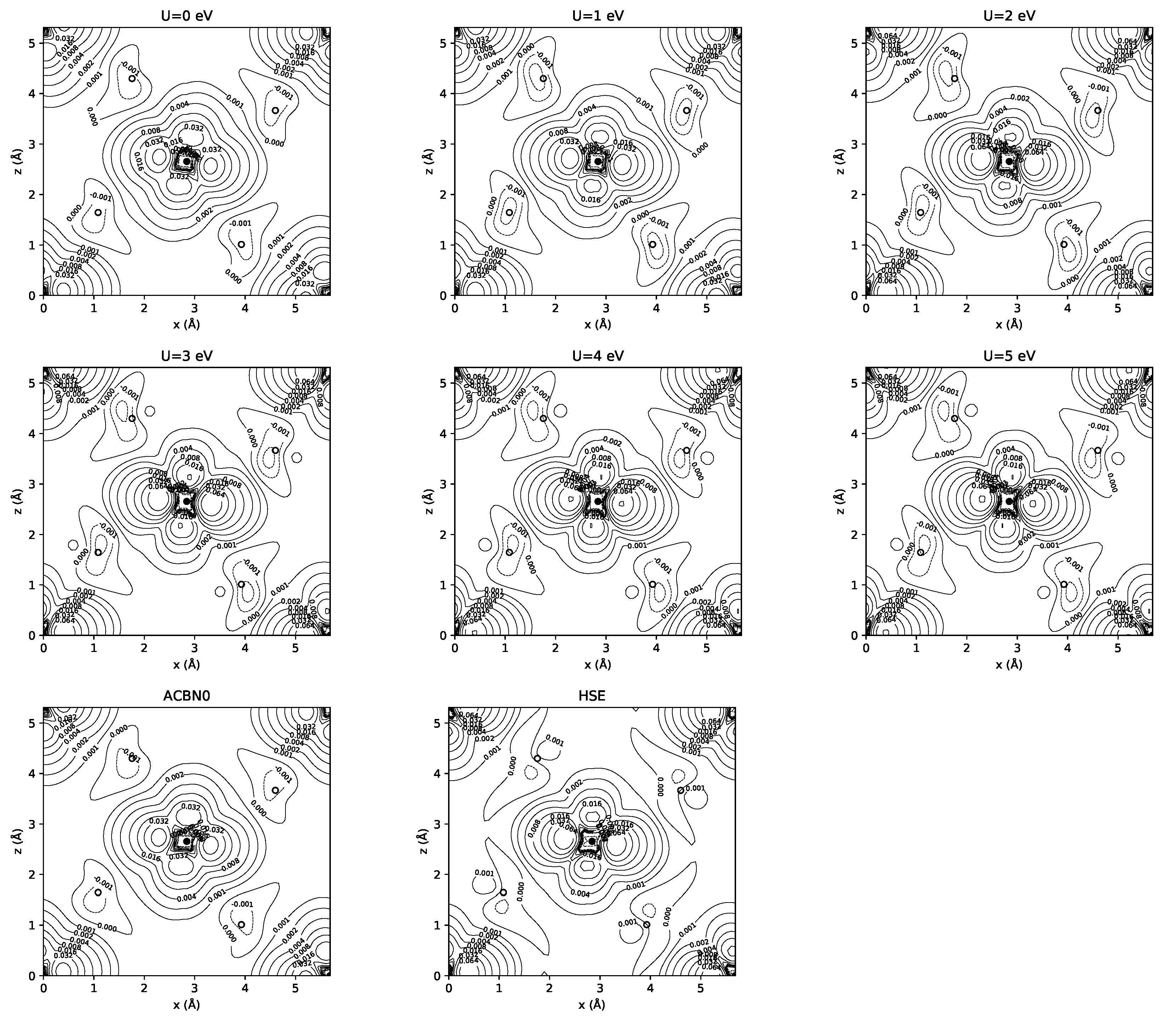
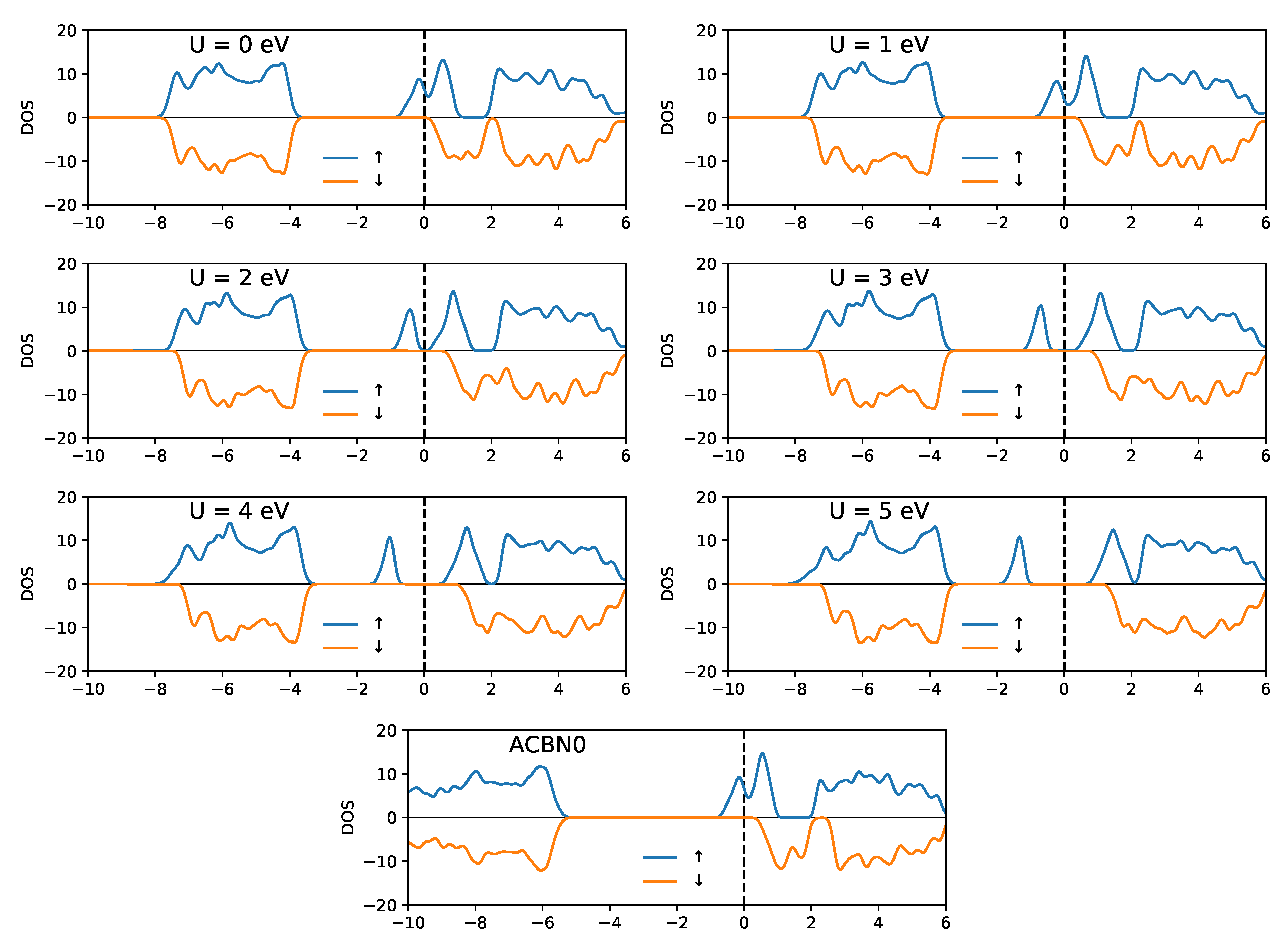
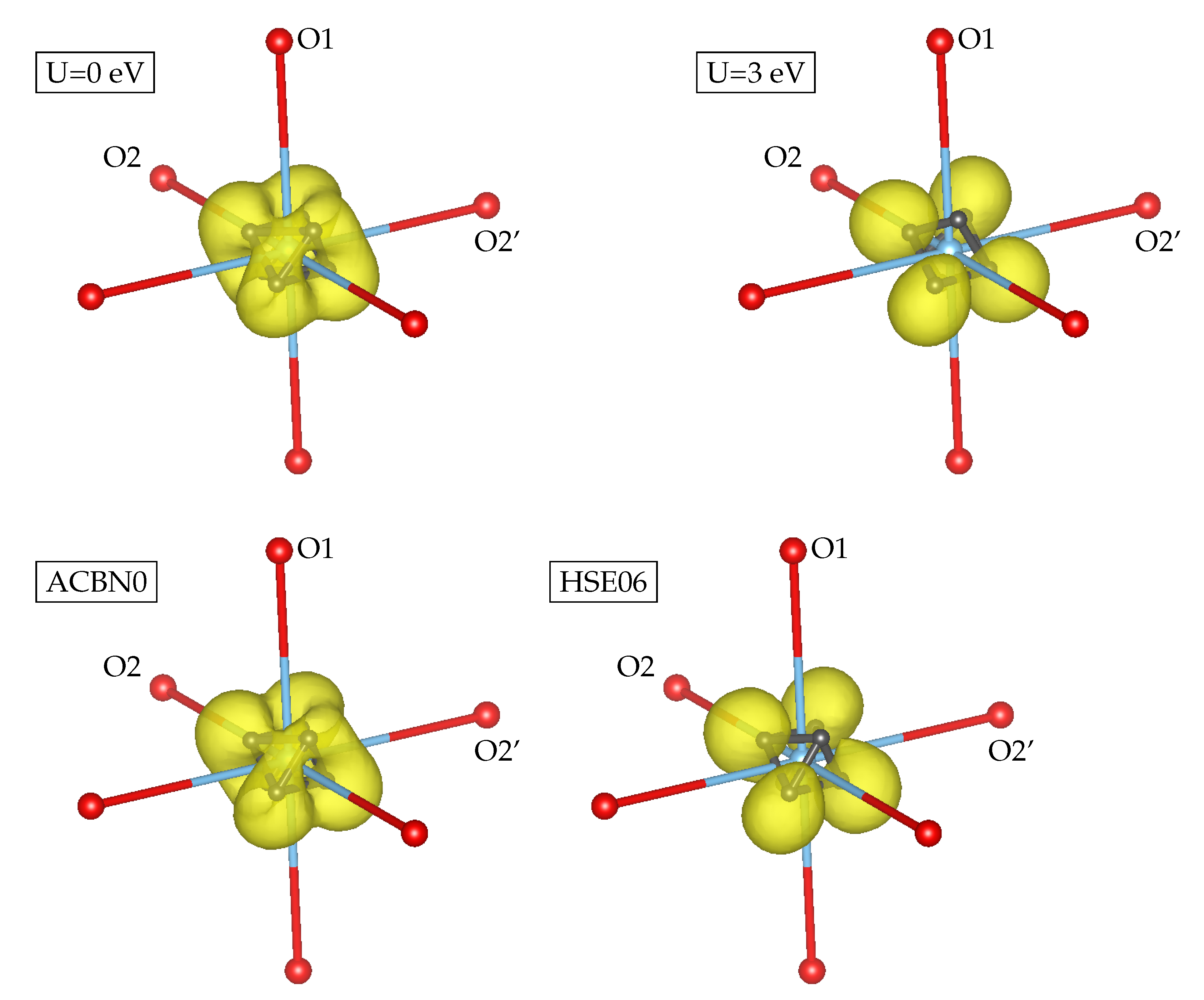
3.1. YTiO
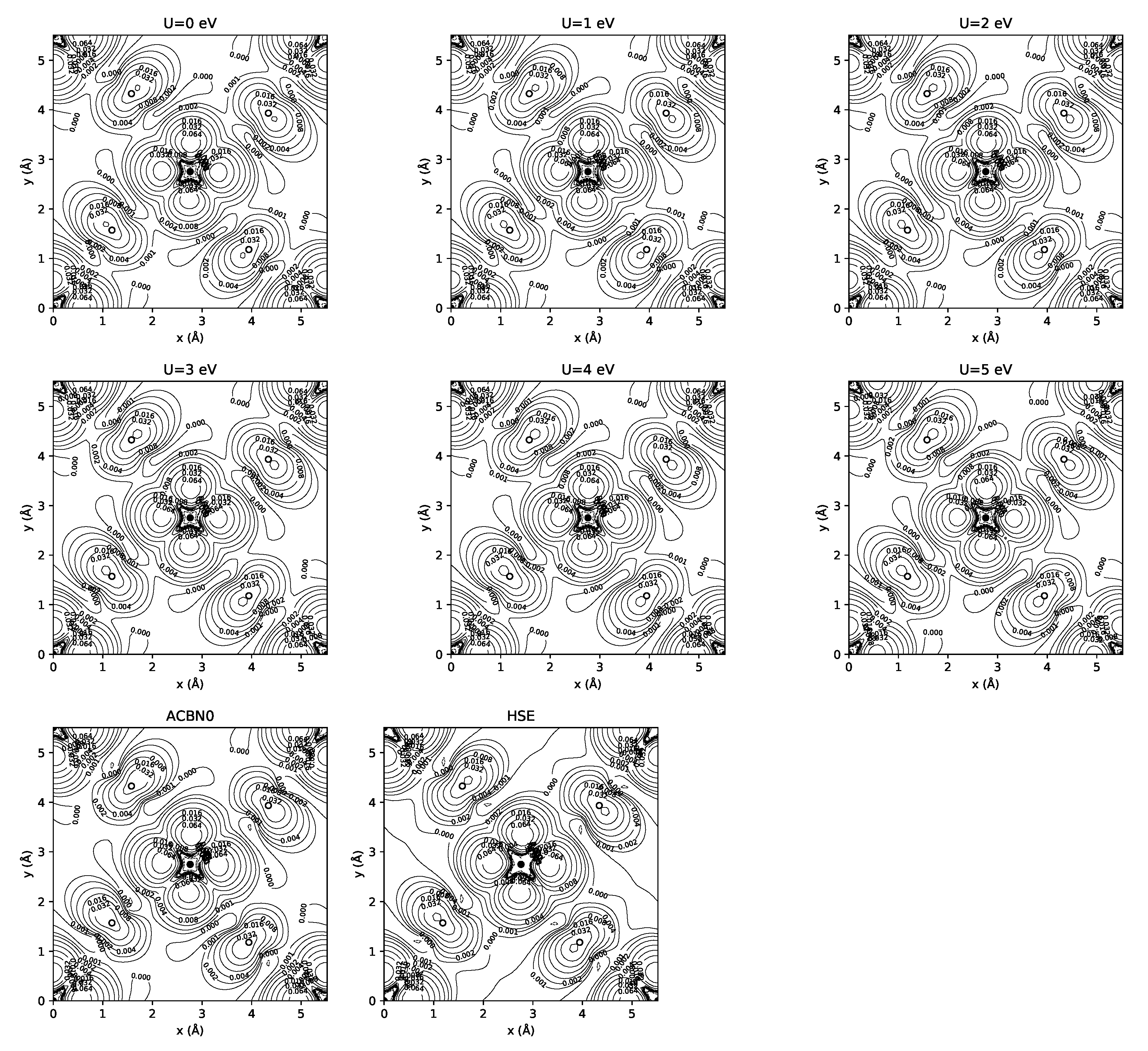
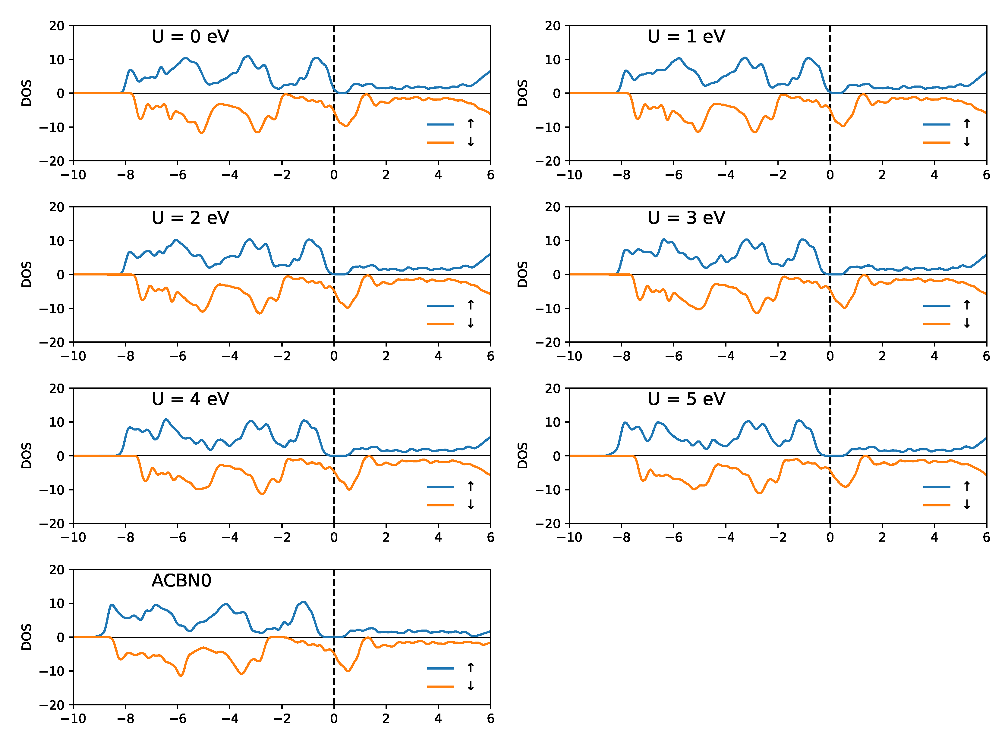
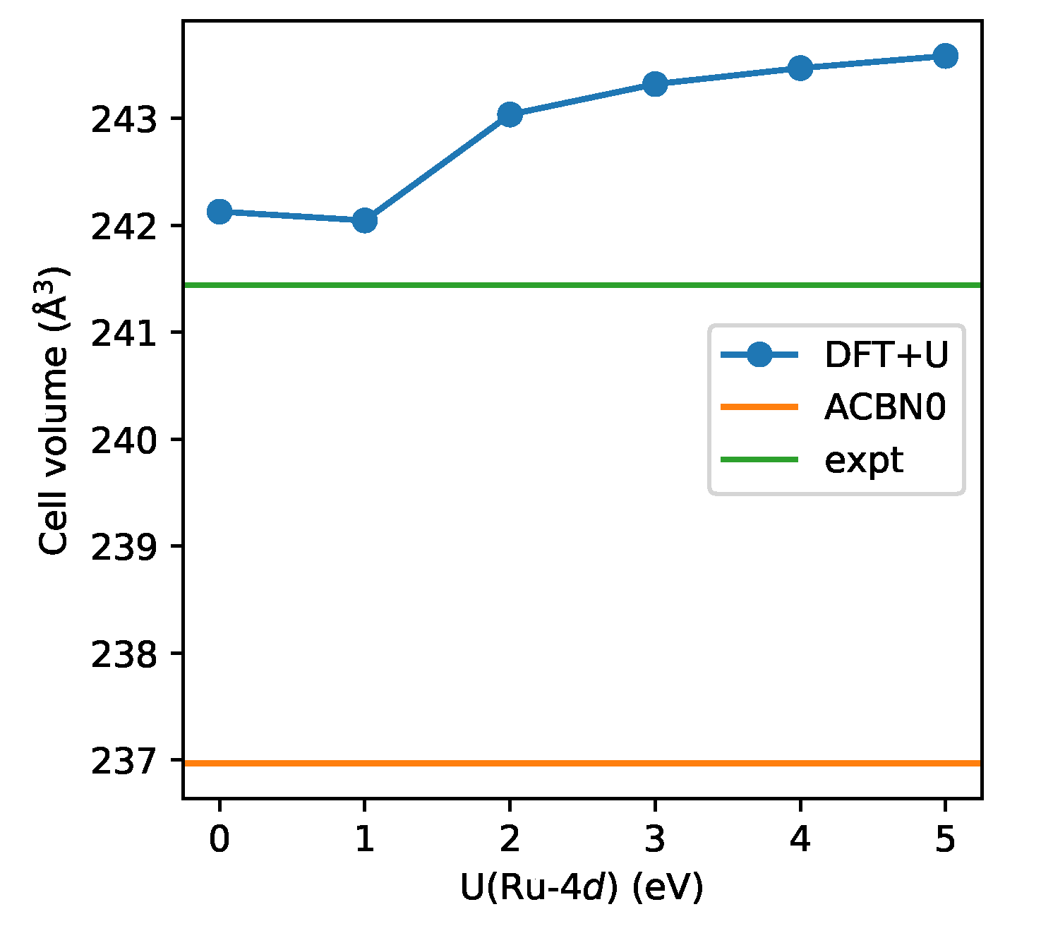
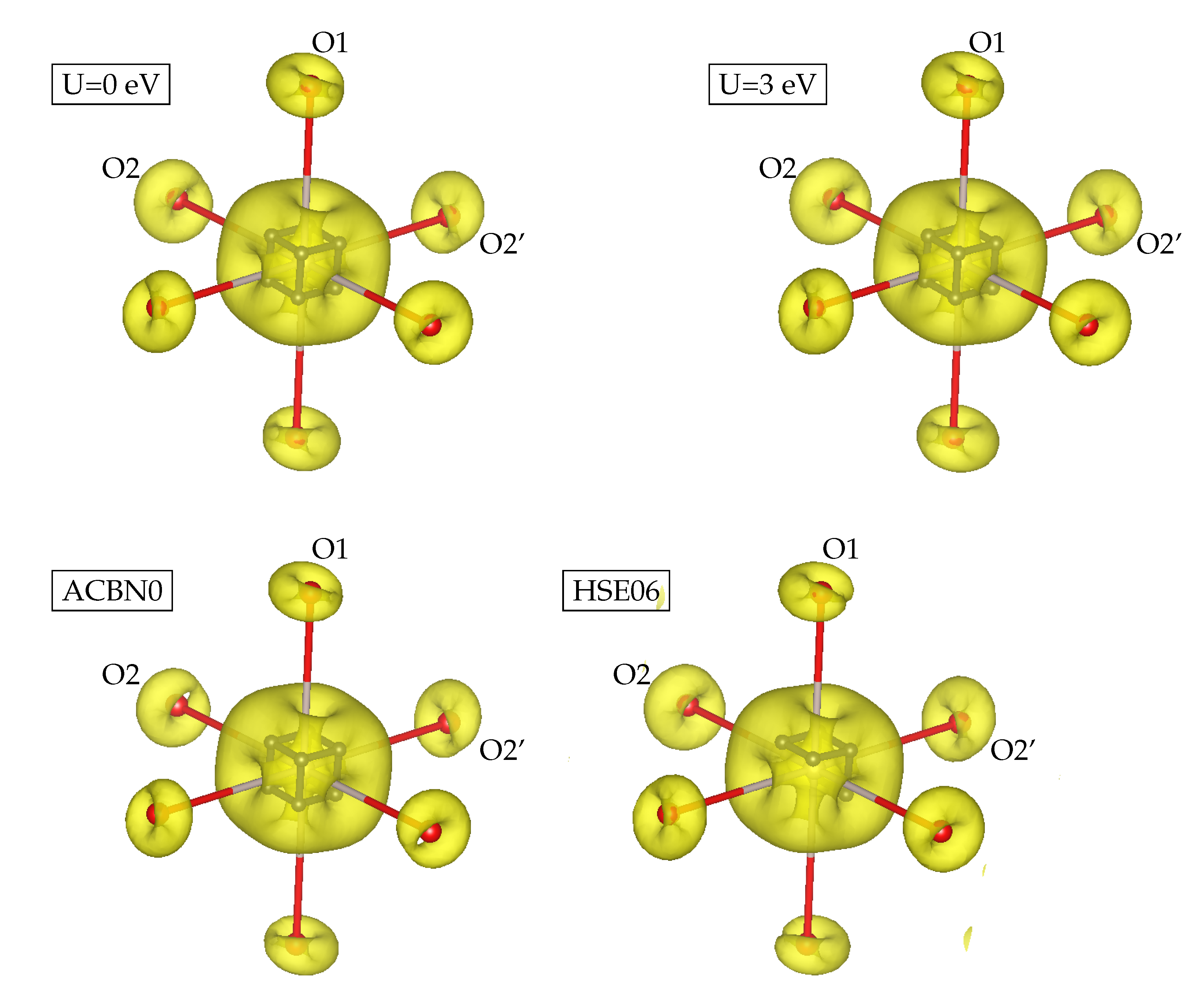
3.2. SrRuO
4. Discussion
5. Conclusions
Author Contributions
Funding
Data Availability Statement
Acknowledgments
Conflicts of Interest
References
- Hohenberg, P.; Kohn, W. Inhomogeneous Electron Gas. Phys. Rev. 1964, 136, B864–B871. [Google Scholar] [CrossRef] [Green Version]
- Kohn, W.; Sham, L.J. Self-Consistent Equations Including Exchange and Correlation Effects. Phys. Rev. 1965, 140, A1133–A1138. [Google Scholar] [CrossRef] [Green Version]
- Perdew, J.P.; Zunger, A. Self-interaction correction to density-functional approximations for many-electron systems. Phys. Rev. B 1981, 23, 5048–5079. [Google Scholar] [CrossRef] [Green Version]
- Tsuneda, T.; Hirao, K. Self-interaction corrections in density functional theory. J. Chem. Phys. 2014, 140, 18A513. [Google Scholar] [CrossRef] [PubMed]
- Petukhov, A.G.; Mazin, I.I.; Chioncel, L.; Lichtenstein, A.I. Correlated metals and the LDA+U method. Phys. Rev. B 2003, 67, 153106. [Google Scholar] [CrossRef] [Green Version]
- Becke, A.D. A new mixing of Hartree–Fock and local density-functional theories. J. Chem. Phys. 1993, 98, 1372–1377. [Google Scholar] [CrossRef]
- Georges, A.; Kotliar, G.; Krauth, W.; Rozenberg, M.J. Dynamical mean-field theory of strongly correlated fermion systems and the limit of infinite dimensions. Rev. Mod. Phys. 1996, 68, 13–125. [Google Scholar] [CrossRef] [Green Version]
- Hedin, L. New Method for Calculating the One-Particle Green’s Function with Application to the Electron-Gas Problem. Phys. Rev. 1965, 139, A796–A823. [Google Scholar] [CrossRef]
- Aryasetiawan, F.; Gunnarsson, O. The GW method. Rep. Prog. Phys. 1998, 61, 237–312. [Google Scholar] [CrossRef] [Green Version]
- Medvedev, M.G.; Bushmarinov, I.S.; Sun, J.; Perdew, J.P.; Lyssenko, K.A. Density functional theory is straying from the path toward the exact functional. Science 2017, 355, 49–52. [Google Scholar] [CrossRef]
- Mezei, P.D.; Csonka, G.I.; Kállay, M. Electron Density Errors and Density-Driven Exchange-Correlation Energy Errors in Approximate Density Functional Calculations. J. Chem. Theory Comput. 2017, 13, 4753–4764. [Google Scholar] [CrossRef] [Green Version]
- Sang, X.; Kulovits, A.; Wang, G.; Wiezorek, J. Validation of density functionals for transition metals and intermetallics using data from quantitative electron diffraction. J. Chem. Phys. 2013, 138, 084504. [Google Scholar] [CrossRef] [PubMed] [Green Version]
- Choudhuri, I.; Truhlar, D.G. Calculating and Characterizing the Charge Distributions in Solids. J. Chem. Theory Comput. 2020, 16, 5884–5892. [Google Scholar] [CrossRef]
- Peng, D.; Nakashima, P.N.H. Measuring Density Functional Parameters from Electron Diffraction Patterns. arXiv 2020, arXiv:2010.09379. [Google Scholar]
- Heyd, J.; Scuseria, G.E.; Ernzerhof, M. Hybrid functionals based on a screened Coulomb potential. J. Chem. Phys. 2003, 118, 8207–8215. [Google Scholar] [CrossRef] [Green Version]
- Cococcioni, M.; de Gironcoli, S. Linear response approach to the calculation of the effective interaction parameters in the LDA+U method. Phys. Rev. B 2005, 71, 035105. [Google Scholar] [CrossRef] [Green Version]
- Agapito, L.A.; Curtarolo, S.; Nardelli, M.B. Reformulation of DFT+U as a Pseudohybrid Hubbard Density Functional for Accelerated Materials Discovery. Phys. Rev. X 2015, 5. [Google Scholar] [CrossRef] [Green Version]
- Gopal, P.; Fornari, M.; Curtarolo, S.; Agapito, L.A.; Liyanage, L.S.I.; Nardelli, M.B. Improved predictions of the physical properties of Zn- and Cd-based wide band-gap semiconductors: A validation of the ACBN0 functional. Phys. Rev. B 2015, 91. [Google Scholar] [CrossRef] [Green Version]
- Gopal, P.; Gennaro, R.D.; dos Santos Gusmao, M.S.; Orabi, R.A.R.A.; Wang, H.; Curtarolo, S.; Fornari, M.; Nardelli, M.B. Improved electronic structure and magnetic exchange interactions in transition metal oxides. J. Phys. Condens. Matter 2017, 29, 444003. [Google Scholar] [CrossRef] [Green Version]
- Bader, R.F.W. A quantum theory of molecular structure and its applications. Chem. Rev. 1991, 91, 893–928. [Google Scholar] [CrossRef]
- Kibalin, I.A.; Yan, Z.; Voufack, A.B.; Gueddida, S.; Gillon, B.; Gukasov, A.; Porcher, F.; Bataille, A.M.; Morini, F.; Claiser, N.; et al. Spin density in YTiO3: I. Joint refinement of polarized neutron diffraction and magnetic x-ray diffraction data leading to insights into orbital ordering. Phys. Rev. B 2017, 96. [Google Scholar] [CrossRef] [Green Version]
- Masys, Š.; Jonauskas, V. On the crystalline structure of orthorhombic SrRuO3: A benchmark study of DFT functionals. Comput. Mater. Sci. 2016, 124, 78–86. [Google Scholar] [CrossRef] [Green Version]
- Kunkemöller, S.; Jenni, K.; Gorkov, D.; Stunault, A.; Streltsov, S.; Braden, M. Magnetization density distribution in the metallic ferromagnet SrRuO3 determined by polarized neutron diffraction. Phys. Rev. B 2019, 100, 054413. [Google Scholar] [CrossRef] [Green Version]
- Giannozzi, P.; Baroni, S.; Bonini, N.; Calandra, M.; Car, R.; Cavazzoni, C.; Ceresoli, D.; Chiarotti, G.L.; Cococcioni, M.; Dabo, I.; et al. Quantum ESPRESSO: A modular and open-source software project for quantum simulations of materials. J. Phys. Condens. Matter 2009, 21, 395502. [Google Scholar] [CrossRef] [PubMed]
- Giannozzi, P.; Andreussi, O.; Brumme, T.; Bunau, O.; Nardelli, M.B.; Calandra, M.; Car, R.; Cavazzoni, C.; Ceresoli, D.; Cococcioni, M.; et al. Advanced capabilities for materials modelling with Quantum ESPRESSO. J. Phys. Condens. Matter 2017, 29, 465901. [Google Scholar] [CrossRef] [PubMed] [Green Version]
- Schlipf, M.; Gygi, F. Optimization algorithm for the generation of ONCV pseudopotentials. Comput. Phys. Commun. 2015, 196, 36–44. [Google Scholar] [CrossRef] [Green Version]
- De-la Roza, A.O.; Johnson, E.R.; Luaña, V. Critic2: A program for real-space analysis of quantum chemical interactions in solids. Comput. Phys. Commun. 2014, 185, 1007–1018. [Google Scholar] [CrossRef]
- Yu, M.; Trinkle, D.R. Accurate and efficient algorithm for Bader charge integration. J. Chem. Phys. 2011, 134, 064111. [Google Scholar] [CrossRef] [Green Version]
- Ruiz, E.; Cirera, J.; Alvarez, S. Spin density distribution in transition metal complexes. Coord. Chem. Rev. 2005, 249, 2649–2660. [Google Scholar] [CrossRef]
- Perdew, J.P.; Ruzsinszky, A.; Csonka, G.I.; Vydrov, O.A.; Scuseria, G.E.; Constantin, L.A.; Zhou, X.; Burke, K. Restoring the Density-Gradient Expansion for Exchange in Solids and Surfaces. Phys. Rev. Lett. 2008, 100, 136406. [Google Scholar] [CrossRef] [Green Version]
- Agapito, L.A.; Fornari, M.; Ceresoli, D.; Ferretti, A.; Curtarolo, S.; Nardelli, M.B. Accurate tight-binding Hamiltonians for two-dimensional and layered materials. Phys. Rev. B 2016, 93, 125137. [Google Scholar] [CrossRef] [Green Version]
- Nardelli, M.B.; Cerasoli, F.T.; Costa, M.; Curtarolo, S.; Gennaro, R.D.; Fornari, M.; Liyanage, L.; Supka, A.R.; Wang, H. PAOFLOW: A utility to construct and operate on ab initio Hamiltonians from the projections of electronic wavefunctions on atomic orbital bases, including characterization of topological materials. Comput. Mater. Sci. 2018, 143, 462–472. [Google Scholar] [CrossRef]
- Lin, L. Adaptively Compressed Exchange Operator. J. Chem. Theory Comput. 2016, 12, 2242–2249. [Google Scholar] [CrossRef] [PubMed] [Green Version]
- Dovesi, R.; Orlando, R.; Erba, A.; Zicovich-Wilson, C.M.; Civalleri, B.; Casassa, S.; Maschio, L.; Ferrabone, M.; Pierre, M.D.L.; D’Arco, P.; et al. CRYSTAL14: A program for the ab initio investigation of crystalline solids. Int. J. Quantum Chem. 2014, 114, 1287–1317. [Google Scholar] [CrossRef]
- Gatti, C.; Saunders, V.R.; Roetti, C. Crystal field effects on the topological properties of the electron density in molecular crystals: The case of urea. J. Chem. Phys. 1994, 101, 10686–10696. [Google Scholar] [CrossRef]
- Himmetoglu, B.; Janotti, A.; Bjaalie, L.; de Walle, C.G.V. Interband and polaronic excitations in YTiO3 from first principles. Phys. Rev. B 2014, 90. [Google Scholar] [CrossRef] [Green Version]
- Varignon, J.; Bibes, M.; Zunger, A. Origin of band gaps in 3d perovskite oxides. Nat. Commun. 2019, 10. [Google Scholar] [CrossRef] [Green Version]
- Jeng, H.T.; Lin, S.H.; Hsue, C.S. Orbital Ordering and Jahn-Teller Distortion in Perovskite Ruthenate SrRuO3. Phys. Rev. Lett. 2006, 97, 067002. [Google Scholar] [CrossRef] [Green Version]
- Ryee, S.; Jang, S.W.; Kino, H.; Kotani, T.; Han, M.J. Quasiparticle self-consistent GW calculation of Sr2RuO4 and SrRuO3. Phys. Rev. B 2016, 93, 075125. [Google Scholar] [CrossRef] [Green Version]
- Yan, Z.; Kibalin, I.A.; Claiser, N.; Gueddida, S.; Gillon, B.; Gukasov, A.; Voufack, A.B.; Morini, F.; Sakurai, Y.; Brancewicz, M.; et al. Spin density in YTiO3: II. Momentum-space representation of electron spin density supported by position-space results. Phys. Rev. B 2017, 96. [Google Scholar] [CrossRef]
- Hansen, N.K.; Coppens, P. Testing aspherical atom refinements on small-molecule data sets. Acta Crystallogr. Sect. A 1978, 34, 909–921. [Google Scholar] [CrossRef]
- Gilmore, C.J.; Shankland, K.; Bricogne, G. Applications of the Maximum Entropy Method to Powder Diffraction and Electron Crystallography. Proc. Math. Phys. Sci. 1993, 442, 97–111. [Google Scholar]
- Volkov, A.; Gatti, C.; Abramov, Y.; Coppens, P. Evaluation of net atomic charges and atomic and molecular electrostatic moments through topological analysis of the experimental charge density. Acta Crystallogr. Sect. A Found. Crystallogr. 2000, 56, 252–258. [Google Scholar] [CrossRef] [PubMed]
- Gatti, C.; Saleh, G.; Presti, L.L. Source Function applied to experimental densities reveals subtle electron-delocalization effects and appraises their transferability properties in crystals. Acta Crystallogr. Sect. B Struct. Sci. Cryst. Eng. Mater. 2016, 72, 180–193. [Google Scholar] [CrossRef]
- May, K.J.; Kolpak, A.M. Improved description of perovskite oxide crystal structure and electronic properties using self-consistent Hubbard U corrections from ACBN0. Phys. Rev. B 2020, 101. [Google Scholar] [CrossRef]
- Ceresoli, D.; Tosatti, E. Pressure-induced insulator-metal and structural transitions of BaBiO3 from first principles LDA+U. In Proceedings of the APS March Meeting Abstact L40.00008, New Orleans, LA, USA, 10–14 March 2008. [Google Scholar]
- Hirshfeld, F.L. Bonded-atom fragments for describing molecular charge densities. Theor. Chim. Acta 1977, 44, 129–138. [Google Scholar] [CrossRef]
- Yuk, S.F.; Pitike, K.C.; Nakhmanson, S.M.; Eisenbach, M.; Li, Y.W.; Cooper, V.R. Towards an accurate description of perovskite ferroelectrics: Exchange and correlation effects. Sci. Rep. 2017, 7. [Google Scholar] [CrossRef]
- Zhang, Y.; Sun, J.; Perdew, J.P.; Wu, X. Comparative first-principles studies of prototypical ferroelectric materials by LDA, GGA, and SCAN meta-GGA. Phys. Rev. B 2017, 96. [Google Scholar] [CrossRef] [Green Version]
- Gautam, G.S.; Carter, E.A. Evaluating transition metal oxides within DFT-SCAN and SCAN+U frameworks for solar thermochemical applications. Phys. Rev. Mater. 2018, 2. [Google Scholar] [CrossRef]
- Jr, V.L.C.; Cococcioni, M. Extended DFT+U+V method with on-site and inter-site electronic interactions. J. Phys. Condens. Matter 2010, 22, 055602. [Google Scholar] [CrossRef] [Green Version]
- Lee, S.H.; Son, Y.W. Efficient First-Principles Approach with a Pseudohybrid Density Functional for Extended Hubbard Interactions. arXiv 2019, arXiv:1911.05967. [Google Scholar]
- Tancogne-Dejean, N.; Rubio, A. Parameter-free hybridlike functional based on an extended Hubbard model: DFT+U+V. Phys. Rev. B 2020, 102. [Google Scholar] [CrossRef]
- James, A.D.N.; Harris-Lee, E.I.; Hampel, A.; Aichhorn, M.; Dugdale, S.B. Wavefunctions, electronic localization and bonding properties for correlated materials beyond the Kohn-Sham formalism. arXiv 2020, arXiv:2010.04694. [Google Scholar]
- Bruno, G.; Macetti, G.; Presti, L.L.; Gatti, C. Spin Density Topology. Molecules 2020, 25, 3537. [Google Scholar] [CrossRef]


| Method | q(Y) | q(Ti) | q(O1) | q(O2) | m(Y) | m(Ti) | m(O1) | m(O2) | Tot. Magn. |
|---|---|---|---|---|---|---|---|---|---|
| U = 0 eV | 2.1101 | 1.9066 | −1.3325 | −1.3423 | 0.0594 | 0.7974 | 0.0521 | 0.0456 | 1.0000 |
| U = 1 eV | 2.1131 | 1.9198 | −1.3387 | −1.3474 | 0.0549 | 0.8161 | 0.0461 | 0.0414 | 1.0000 |
| U = 2 eV | 2.1182 | 1.9336 | −1.3448 | −1.3537 | 0.0457 | 0.8348 | 0.0396 | 0.0399 | 1.0000 |
| U = 3 eV | 2.1220 | 1.9496 | −1.3510 | −1.3605 | 0.0376 | 0.8511 | 0.0342 | 0.0386 | 1.0000 |
| U = 4 eV | 2.1243 | 1.9671 | −1.3574 | −1.3673 | 0.0316 | 0.8647 | 0.0299 | 0.0369 | 1.0000 |
| U = 5 eV | 2.1255 | 1.9854 | −1.3636 | −1.3739 | 0.0272 | 0.8764 | 0.0264 | 0.0350 | 1.0000 |
| ACBN0 | 2.2678 | 2.0992 | −1.4481 | −1.4597 | 0.0450 | 0.8208 | 0.0458 | 0.0442 | 1.0000 |
| HSE06 | 2.2343 | 2.0259 | −1.4127 | −1.4239 | 0.0273 | 0.8513 | 0.0369 | 0.0422 | 1.0000 |
| expt. PND | N/A | N/A | N/A | N/A | -0.047 | 0.715 | 0.016 | 0.004 | 0.704 |
| PBE0 | N/A | N/A | N/A | N/A | 0.015 | 0.852 | 0.036 | 0.049 | 0.998 |
| Method | q(Sr) | q(Ru) | q(O1) | q(O2) | m(Sr) | m(Ru) | m(O1) | m(O2) | Tot. Magn. |
|---|---|---|---|---|---|---|---|---|---|
| U = 0 eV | 1.5745 | 1.6715 | −1.0795 | −1.0872 | 0.0136 | 1.3898 | 0.1942 | 0.1853 | 1.9772 |
| U = 1 eV | 1.5754 | 1.6576 | −1.0750 | −1.0832 | 0.0136 | 1.3967 | 0.1988 | 0.1909 | 1.9989 |
| U = 2 eV | 1.5763 | 1.6423 | −1.0703 | −1.0784 | 0.0134 | 1.3869 | 0.2025 | 0.1946 | 2.0000 |
| U = 3 eV | 1.5773 | 1.6263 | −1.0653 | −1.0733 | 0.0134 | 1.3740 | 0.2068 | 0.1990 | 2.0000 |
| U = 4 eV | 1.5783 | 1.6098 | −1.0601 | −1.0682 | 0.0134 | 1.3597 | 0.2115 | 0.2040 | 2.0000 |
| U = 5 eV | 1.5793 | 1.5927 | −1.0555 | −1.0612 | 0.0136 | 1.3436 | 0.2163 | 0.2102 | 2.0000 |
| ACBN0 | 1.6214 | 1.8594 | −1.1581 | −1.1649 | 0.0086 | 1.5103 | 0.1623 | 0.1565 | 2.0000 |
| HSE06 | 1.6608 | 2.1080 | −1.2576 | −1.2539 | −0.0023 | 1.4989 | 0.1801 | 0.1432 | 2.0000 |
| expt. 2 K S + L | N/A | N/A | N/A | N/A | N/A | 1.35 | 0.20 | 0.20 | 1.95 |
| expt. 2 K S | N/A | N/A | N/A | N/A | N/A | 1.42 | 0.20 | 0.20 | 2.02 |
| other DFT (PBE) | N/A | N/A | N/A | N/A | N/A | 1.34 | 0.16 | 0.13 | 1.79 |
Publisher’s Note: MDPI stays neutral with regard to jurisdictional claims in published maps and institutional affiliations. |
© 2021 by the authors. Licensee MDPI, Basel, Switzerland. This article is an open access article distributed under the terms and conditions of the Creative Commons Attribution (CC BY) license (http://creativecommons.org/licenses/by/4.0/).
Share and Cite
Menescardi, F.; Ceresoli, D. Comparative Analysis of DFT+U, ACBN0, and Hybrid Functionals on the Spin Density of YTiO3 and SrRuO3. Appl. Sci. 2021, 11, 616. https://doi.org/10.3390/app11020616
Menescardi F, Ceresoli D. Comparative Analysis of DFT+U, ACBN0, and Hybrid Functionals on the Spin Density of YTiO3 and SrRuO3. Applied Sciences. 2021; 11(2):616. https://doi.org/10.3390/app11020616
Chicago/Turabian StyleMenescardi, Francesca, and Davide Ceresoli. 2021. "Comparative Analysis of DFT+U, ACBN0, and Hybrid Functionals on the Spin Density of YTiO3 and SrRuO3" Applied Sciences 11, no. 2: 616. https://doi.org/10.3390/app11020616