Article

Video Forensics: Identifying Colorized Images Using Deep Learning

Faculty of Engineering, Universidad Militar Nueva Granada, 110111 Bogotá, Colombia
*
Author to whom correspondence should be addressed.
Appl. Sci. 2021, 11(2), 476; https://doi.org/10.3390/app11020476
Submission received: 16 December 2020 / Revised: 31 December 2020 / Accepted: 2 January 2021 / Published: 6 January 2021
(This article belongs to the Section Computing and Artificial Intelligence)

Abstract

:

Featured Application

This paper presents two CNN-based models (custom and by transfer learning) for the task of classifying colorized and original images and includes an assessment of the impact of three hyperparameters: image size, optimizer, and dropout value. The models are compared with each other in terms of performance and inference times and with some state-of-the-art approaches.

Abstract

In recent years there has been a significant increase in images and videos circulating in social networks and media, edited with different techniques, including colorization. This has a negative impact on the forensic field because it is increasingly difficult to discern what is original content and what is fake. To address this problem, we propose two models (a custom architecture and a transfer-learning-based model) based on CNNs that allows a fast recognition of the colorized images (or videos). In the experimental test, the effect of three hyperparameters on the performance of the classifier were analyzed in terms of HTER (Half Total Error Rate). The best result was found for the Adam optimizer, with a dropout of 0.25 and an input image size of 400 × 400 pixels. Additionally, the proposed models are compared with each other in terms of performance and inference times and with some state-of-the-art approaches. In terms of inference times per image, the proposed custom model is 12x faster than the transfer-learning-based model; however, in terms of precision (P), recall and F1-score, the transfer-learning-based model is better than the custom model. Both models generalize better than other models reported in the literature.

1. Introduction

Image and video are some of the most used forms of communication thanks to the evolution of mobile technologies and the appearance of smartphones and social networks such as Facebook and Instagram. This growing popularity of digital media, together with the easy access to image editing tools, has facilitated the counterfeiting of this type of content. It is estimated that in 2020 more than 1.4 billion pictures were taken [1], which could be edited for different uses such as entertainment, as in the film and advertising sectors. Tools such as Photoshop, Affinity Photo, and Paintshop allow for simple, manual image editing without a trace visible to the human eye. Another editing approach is the automatic generation of tampered data through deep learning algorithms with CNNs (Convolutional Neural Network) [2] or GANs (Generative Adversarial Networks) [3]. In addition, fake images or videos can also be used for malicious purposes, impacting political, social, legal (e.g., forensic field) and moral environments, bearing in mind that the manipulation affects their content [4].
Specifically, in the forensic field, digital content such as image and video can become digital evidence within a legal process, in which this type of data helps to confirm the facts under examination. Thus, if the digital evidence has been intentionally manipulated, it can directly affect the course of the investigation.
Among the methods of image and video editing that negatively impact the forensic field are:
  • Copy/move: consisting of copying a part of the image and pasting it over the same image. In this way, a specific area of the image can be hidden (for example, a weapon).
  • Cut/paste and splicing: consisting of cutting an object from one image and copying it to another image or creating an image with the contents obtained from two different images, respectively. It has the same effect of hiding a specific area of the image as copy/move or even creating a new scene.
  • Retouching: this method alters certain characteristics of the image, through techniques such as blurring. An object may appear blurry in the edited image, making it difficult to identify.
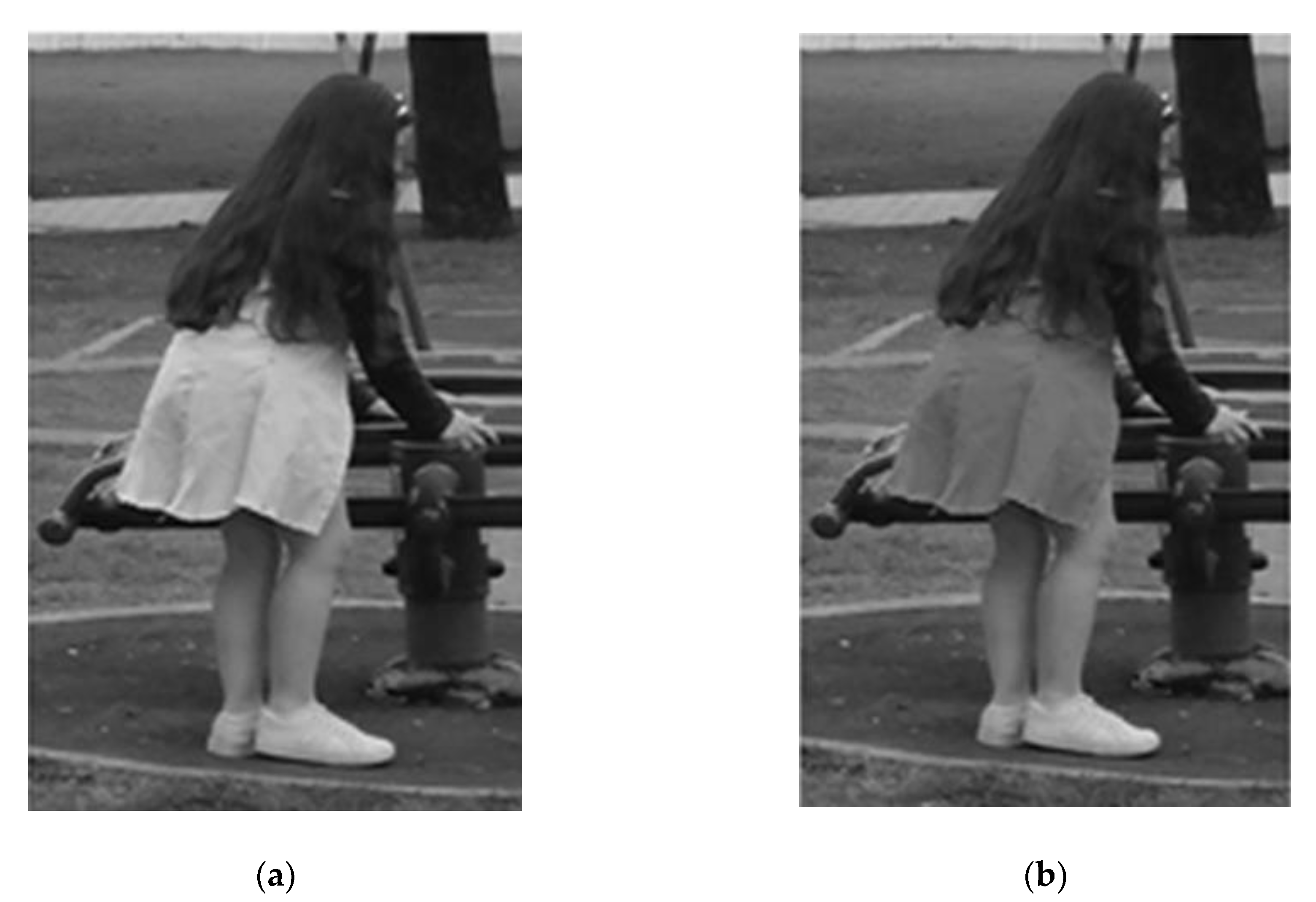
  • Colorization: unlike the previous types of manipulation, the original objects in the image are not hidden, blurred or new, but their color intensities are modified. The impact on the forensic video field is that the version of a witness may differ from the tampered evidence, for example, in clothing colors, skin color or vehicle color, among others.
It is colorization that has had the greatest boom in recent years. In manual colorization (Figure 1), the color of the image is altered in specific areas using tools such as Photoshop [5,6]; while in automatic colorization with deep learning, pairs of grayscale and color images are used to train the models that will later allow them to color images and videos that are initially in grayscale [7,8,9].
The counterpart of the generation corresponds to the identification of fake image or video. In the forensic field, it is essential to know if an image or video is authentic, to make that content admissible as digital evidence. In the literature there are many proposals about tampered recognition using active techniques such as watermarking [10,11] and to a lesser extent works based on passive techniques such as deep learning (DL) [12,13,14,15,16]. The major limitation of DL-based approaches is the need for large image datasets to carry out model training, whose diversity should include different file formats (e.g., JPEG, TIF, BMP), sizes, color depth (24-bit, 8-bit, 1 bit per pixel), and type of manipulation (manual and automatic). In addition, in the case of emerging techniques such as colorization, there are few open-access image or video datasets for this purpose.
Some hand-crafted approaches such as the Fake Colorized Image Detection (FCID-HIST and FCID-FE) methods, which are based on histograms and feature coding, highlight the problem of generalization, i.e., they have a significant decrease in performance between the results of internal and external validation [17]. Specifically, for the FCID-HIST method, the result of internal validation in terms of HTER (Half Total Error Rate) is 24.45%, and for external validation it is up to 41.85%. It is pointed out that the lower the HTER value, the better. That is, for the FCID-HIST method you have significantly more misclassifications in the case of external validation. A similar behavior occurs with the FCID-FE method.
On the other hand, CNN-based architectures such as WISERNet, specifically designed for the recognition of colorized images, also had problems of generalization [14,15]. For example, the HTER value in internal validation is 0.95%, but for external validation it increases significantly to 22.55%. Using a different dataset, internal validation achieved an HTER of 1.1%, and external validation of 16.6%.
Considering that the diversity of training data affects the performance of the classifier, this research addresses the problem of generalization. The main contributions of this research are focused on the following topics:
  • A custom architecture and a transfer-learning-based model for the classification of colorized images are proposed.
  • The impact of the training dataset is evaluated. Three options are used, one with a single and small public dataset and the other mixing two public datasets but varying the number of images.
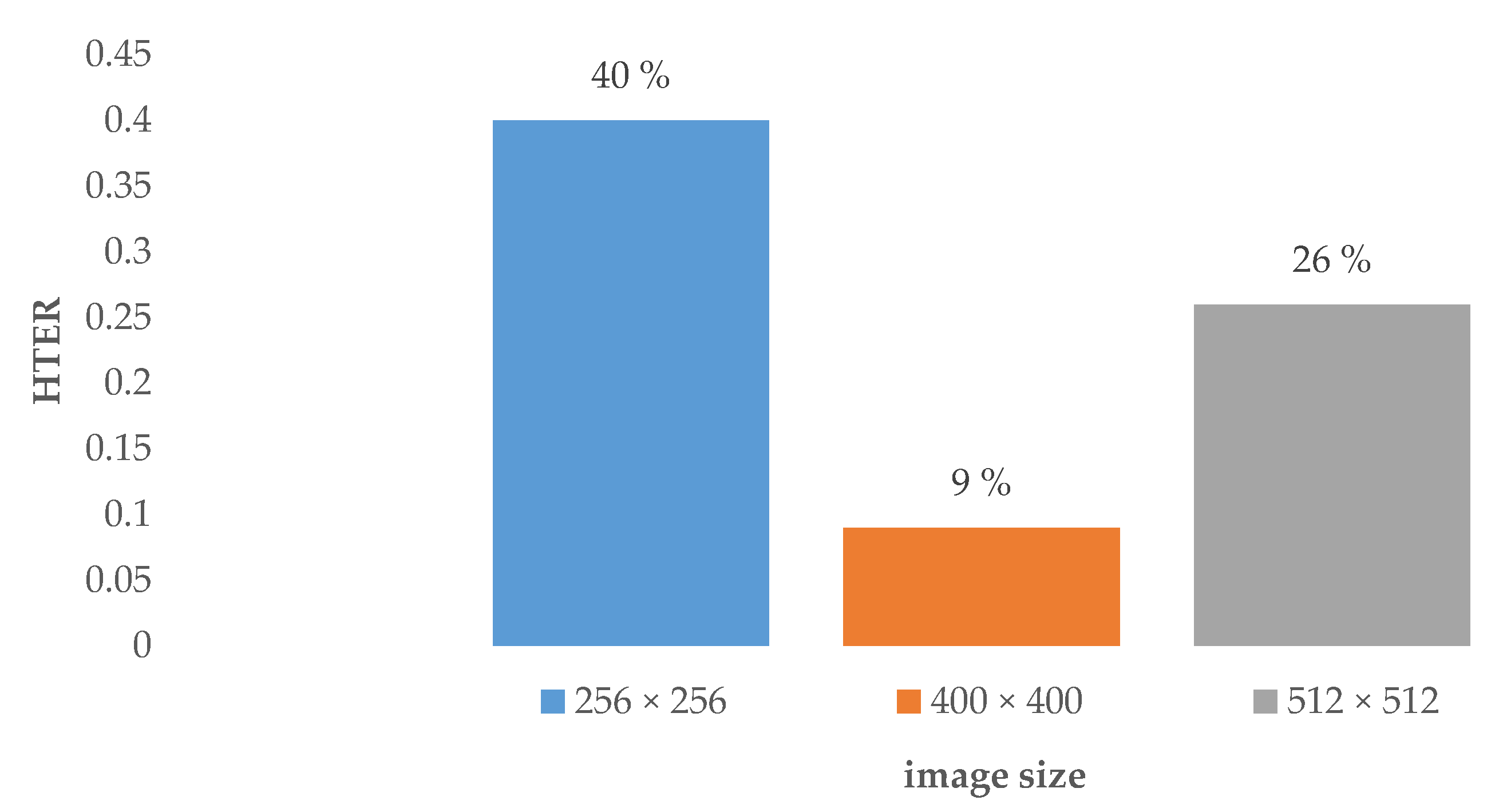
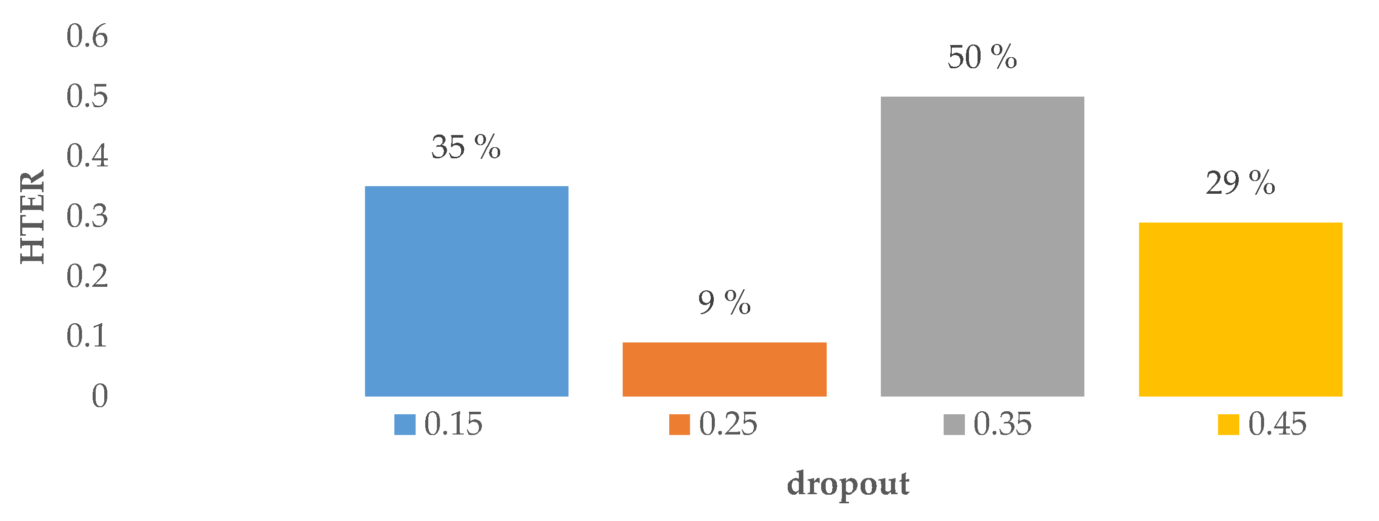
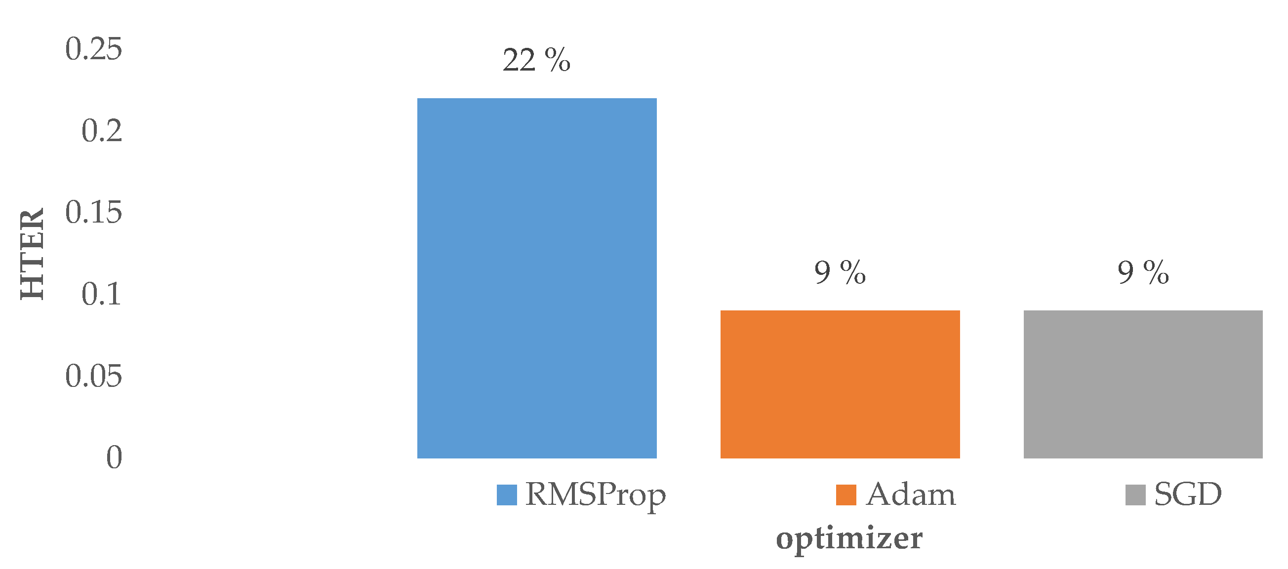
  • Detailed results related to classifier performance for different image sizes, optimizers, and dropout values are provided.
  • In addition, the results of the custom model are compared with a VGG-16-based model (transfer learning) in terms of evaluation metrics as well as training, and inference times.
The rest of the document is organized as follows. Section 2 explains the proposed custom model and the proposed transfer-learning-based model. Section 3 describes the design of the experimental tests. Section 4 shows the impact of the hyperparameters on the custom model and the VGG-16-based model. Section 5 shows the results and the comparison between the custom model, the transfer-learning-based model, and some state-of-the-art architectures. Finally, the research is concluded in Section 6.

2. Proposed Models

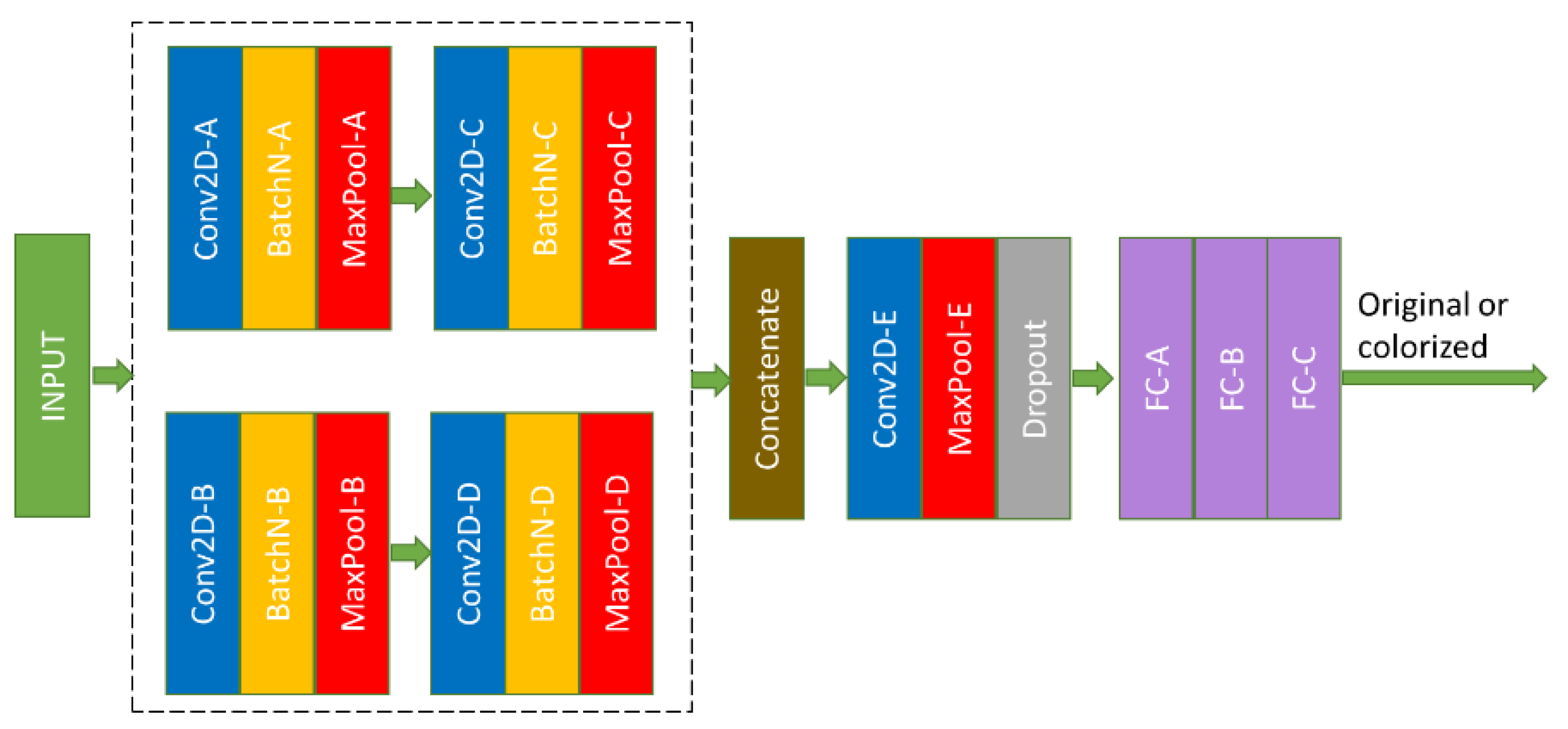
2.1. The Proposed Custom Model

The proposed architecture has two parallel paths that allows convolutions to the input image with different kernel sizes and numbers of filters. It has a shallow depth, with only three convolutional layers and three fully-connected (FC) layers. Each path includes two convolutional layers each followed by batch normalization and max-pooling layers. The two parallel paths are concatenated to enter a new convolution layer followed by a max-pooling layer. The network is then flattened and followed by three FC layers of 400, 200, and 2 outputs, respectively. Figure 2 shows the proposed architecture and Table 1 summarizes the network structure. The custom model has about 16 million parameters.
As can be seen in Table 1, the kernel and the number of filters of each convolutional layer in the parallel block varies between the two branches. In one branch, the architecture makes use of a simple technique to reduce dimensionality of the input color image through 1 × 1 convolutions, preserving its most outstanding properties. In the other branch, the architecture uses 3 × 3 convolutions to extract patterns with a different resolution to those of the first branch. Since shape patterns are not important for this type of classification problem, the network is not very deep.
The ReLU activation function is applied in all convolutional and FC layers (except the last layer). It was selected because it is an efficient function which has been widely used in CNNs for classification tasks [18]. The output is obtained through Equation (1):
ReLU(x) = max(0,x),
where x is the result of the convolution (or the weighted sum, in the case of FC layers). With the ReLU function application, all values of the feature maps are positive. On the other hand, the output layer uses the softmax function instead of the sigmoid function because the proposed architecture has two units in the output to ensure compatibility with the TensorFlow method to calculate the F1-score (i.e., tfa.metrics.F1Score).
To evaluate the size of the input image, three different resolutions were selected. Finally, regarding the optimizer, RMSProp, SGD and Adam were selected to analyze their impact on classifier performance.

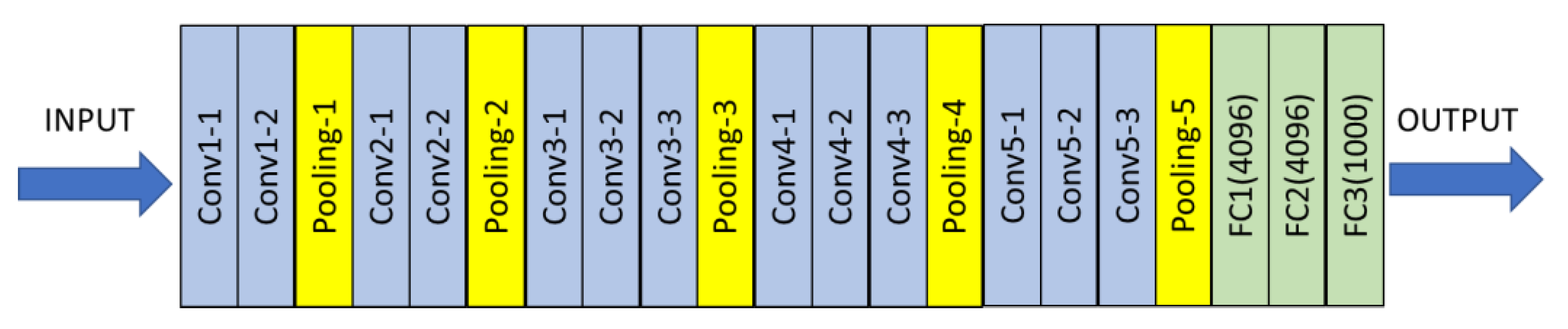
2.2. The Proposed Transfer-Learning-Based Model

VGG-16 is a pre-trained CNN for the object classification task proposed by K. Simonyan and A. Zisserman in 2014 [19]. This network was trained with the ImageNet dataset which includes more than 14 million images belonging to 1000 different classes. VGG was the winning network in the 2014 ImageNet Large-Scale Visual Recognition Challenge (ILSVRC 2014) in the classification + location category in terms of location error and was ranked second in terms of classification error [20]. It is composed of 13 convolutional layers and 3 fully connected layers with 4096, 4096 and 1000 outputs, respectively (Figure 3). It has more than 130 million parameters.
VGG-16 has been widely used for classification tasks by means of transfer learning [21,22]. One of the transfer-learning alternatives is to freeze the filter weights up to a specific layer in the network discarding the other layers, and then adding new fully connected layers to the frozen network. Therefore, the trainable parameters are only those corresponding to the FC layers (since the others are transferred from the pre-trained model).
In this case, the last pooling layer (i.e., pooling_5) was selected to transfer the pre-trained weights to the new model. Like the original network, three FC layers were added, but with a lower number of outputs because the total classes of the current problem are significantly smaller than those of the original problem. Specifically, the three FC layers have 512, 200 and 2 units, respectively. Before the last FC layer, we add a dropout of 0.25. The last layer does not have one unit (unlike typical binary classification problems) but two outputs to improve compatibility with the F1 method of Tensorflow add-ons. The number of parameters in the transfer-learning-based model is lower than the pre-trained VGG-16 due to the reduction of units in the FC layers. In fact, the proposed transfer-learning-based model has about 82 million parameters.

3. Experiments

To objectively evaluate the predictive performance of the proposed network, we carried out the following experiments:
  • Train and validate the custom architecture and the transfer-learning-based model with three different data sets.
  • Measure the impact of some hyperparameters (image size, optimizer and dropout) on the performance of the custom model.
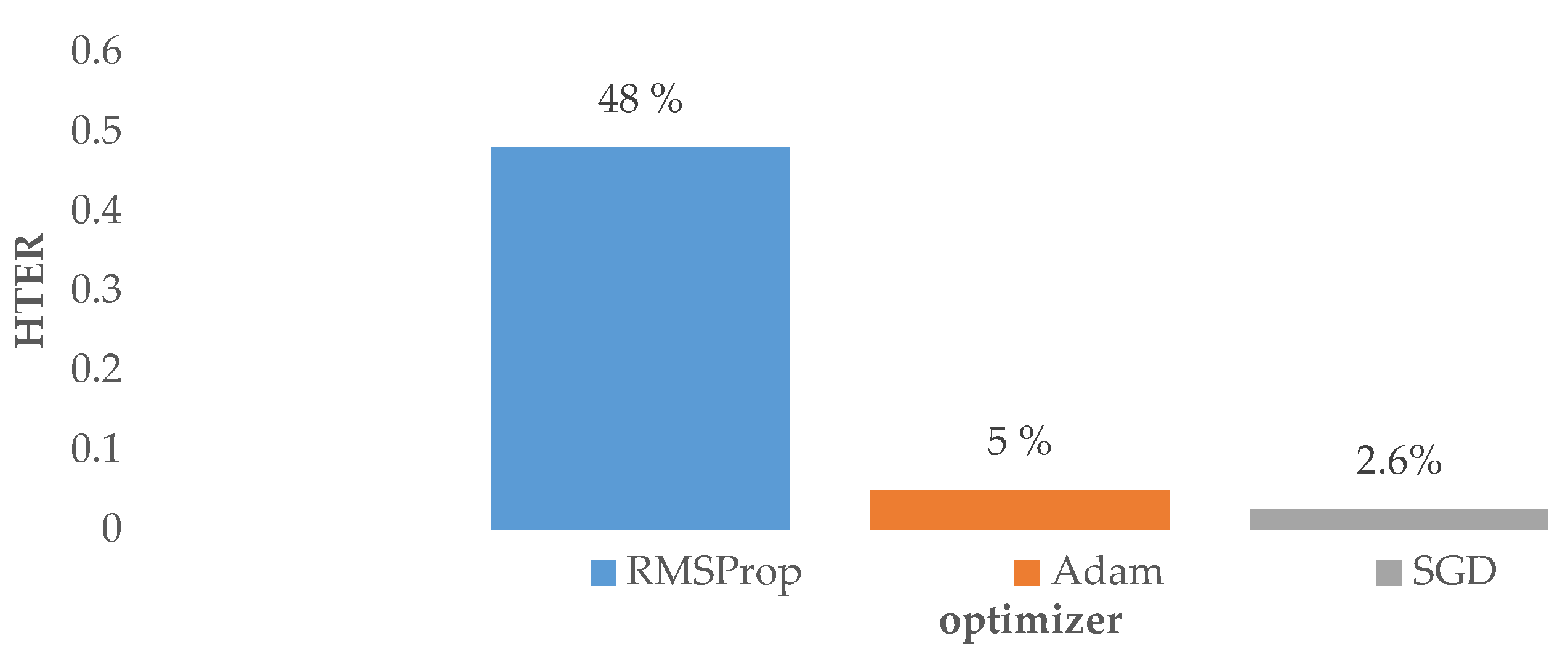
  • Transfer learning from a VGG-16 pre-trained model with new fixed FC layers but varying the optimizer.
  • Calculate the training and inference times of the custom model as well as the transfer-learning-based model.

3.1. Datasets

To train and validate the proposed architectures, three different datasets (DA, DB, DC) were used to analyze the impact of data diversity on classifier performance. The dataset DA contains 331 original images with their corresponding colorized forgeries obtained from the CG-1050 dataset [5,6]. The colorized images were created manually with Photoshop, manipulating the color of specific objects in the image. It contains both color and grayscale images for each pair of original vs. colorized image. This dataset was divided into three subgroups: training (80%), validation (10%) and external test (10%).
The second dataset, DB, is composed of images from both the CG-1050 and Learning Representations for Automatic Colorization (LRAC), specifically ctest10k [23]. From the CG-1050 we have extracted 331 manually colorized images and 331 original images, while from the LRAC we have selected 4388 automatically colorized images; therefore, the DB contains 4719 colorized images. To adjust the number of original images to allow a class-balanced dataset, 4388 original images were added from a personal repository. In this case, the distribution of the dataset was: 60% for training, 20% for validation and 20% for external test.
Finally, DC contains 9506 original images and 9506 colorized images. Like DB, the colorized images come from CG-1050 (331 images) and LRAC (9175). Again, personal repository images were added to have a class-balanced dataset. The same distribution of images between training, validation and test was used as in DB. Table 2 shows the summary of the main characteristics of each dataset. In all cases, we have grayscale and color images, with different sizes and format.

3.2. Evaluation Metrics

The results of the proposed models were compared using four performance metrics: precision, recall, F1-score and HTER. The last one is a metric widely used in colorization recognition task. From the confusion matrix, precision (P), recall (R), F1-score and HTER are obtained as shown in Equations (2)–(5).
P =   TP / ( TP + FP ) ,
R =   TP / ( TP + FN ) ,
F 1 = 2   ( P R ) / ( P + R ) ,
HTER = FP TN + FP + FN TP + FN 2 ,
In the current problem, TP corresponds to colorized images correctly classified, TN corresponds to original images correctly classified, FN corresponds to colorized images classified as original images, and FP corresponds to original images classified as colorized images. The ideal value of P, R and F1-score is 1, and their worst performance value is 0. In contrast, the ideal HTER value is 0 and the worst performance is 1. Additionally, the best model is not only the one with the highest F1-score and the lowest HTER, but also the one with a good balance between P and R.

3.3. Experimental Hyperparameters of the Custom Model and the VGG-16-Based Model

In CNNs there are two types of hyperparameters, the first related to the network structure and the second to the training algorithm. Among the former are image size, number of convolutional layers, number of filters per layer, stride and padding values, pooling layers, activation functions, data normalization type, number of fully-connected layers, number of units per layer or dropout value. The second category includes optimizer, learning rate, epochs or cost function. From the above, we selected for this test the following: dropout and image size (for network structure) and optimizer (for training algorithm). Table 3 shows the options of the experimental hyperparameters for the custom network which include three image sizes, four dropout values and three optimizer methods.
On the other hand, the VGG-16-based architecture was trained again considering three different optimizers (RMSProp, SGD and Adam) to calculate the trainable parameters (related to the FC layers), obtaining three different models.
In the selection of the optimizer, we used as a reference an article in which the performance of several optimizers is compared in the classification of four known datasets (i.e., MNIST, CIFAR-10, Kaggle Flowers and LFW) with different networks [24]. No single algorithm was the best in all cases. Specifically, for the LFW dataset and the CNN-1 network, the best results were found for RMSProp and Adam. Therefore, the selected optimizers are SGD, RMSProp and Adam, for the following reasons:
  • SGD (i.e., stochastic gradient descent) is one of the most widely used optimizers in machine learning algorithms. However, it has difficulties in terms of time requirements for large datasets.
  • RMSProp is part of the optimization algorithms with an adaptive learning rate (α), which divides it by an exponentially decaying average of squared gradients.
  • Adam is one of the most widely used algorithms in deep learning-based applications. It calculates individual α for different parameters. Unlike SGD, it is computationally efficient [24].
Both for the custom model and the VGG-16-based model, the values of the learning rates are 0.01 for SGD, and 0.001 for both Adam and RMSProp.
Their performance of the proposed nets is presented in the following section.

4. Dataset and Hyperparameter Selection

This section shows the selection of the dataset and some hyperparameters for the custom model and the transfer-learning-based model. The first part is related to the impact of the dataset, the second and third parts are focused on the impact of input image size, dropout and optimizer.

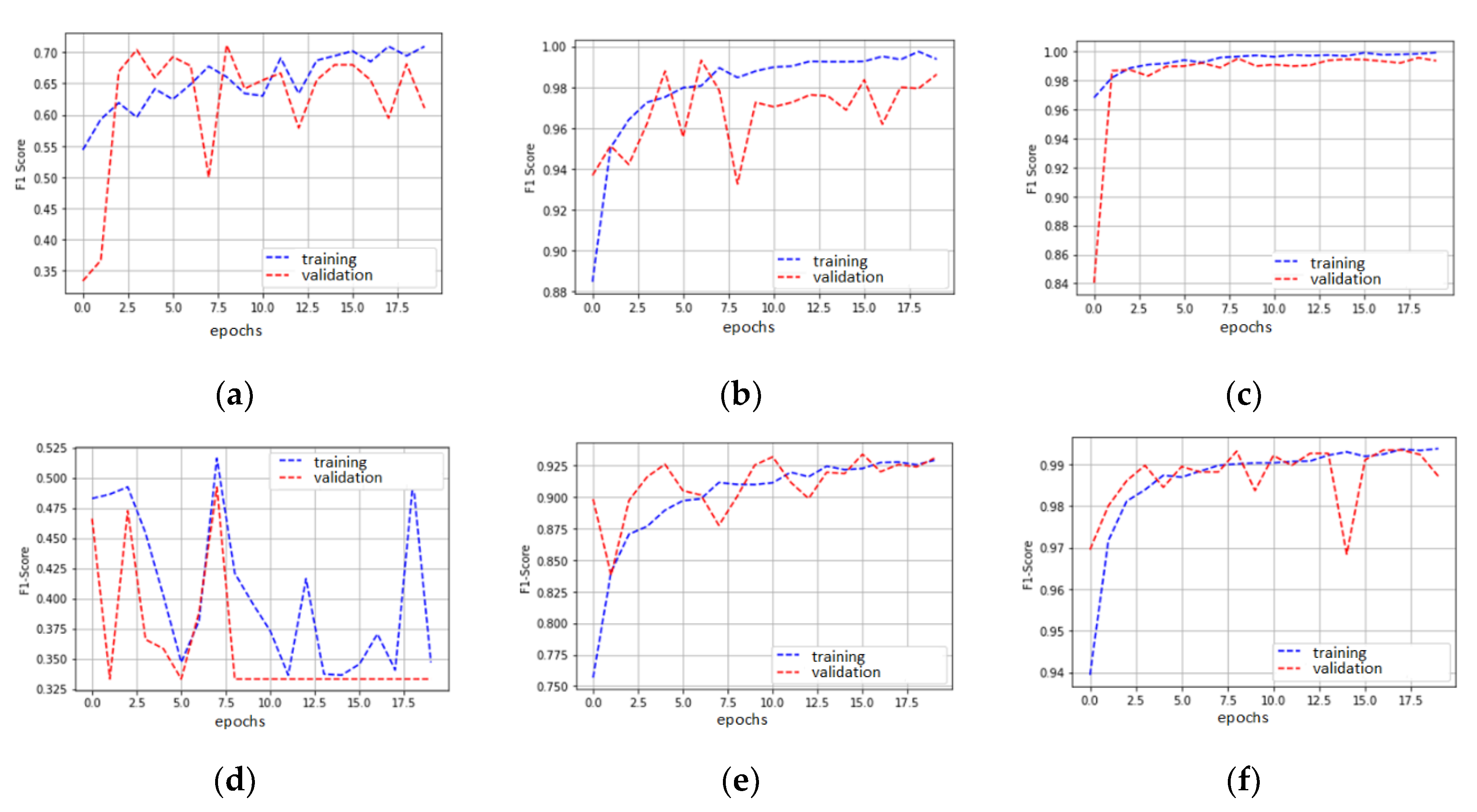
4.1. Impact of the Dataset

To objectively evaluate the impact of the dataset in the colorized image classification task, we trained and validated the custom architecture and the VGG-16-based model with the three datasets, DA, DB and DC. In this test, all hyperparameters were set to the same value for the training stage. Figure 4 shows the performance curves for training and validation using each dataset. The number of epochs in each case was adjusted to 20.
According to Figure 4, when the nets are trained with DA, the F1 score is lower than 0.72, but, if the architecture is trained with DB or DC, the F1 scores are close to 1. Nevertheless, it should be noted that the best performance in the three cases evaluated is obtained with the third dataset, this is because both curves (training and validation) grow and approach each other as the number of epochs increases, so there is no overfitting. Therefore, the DC dataset was used for subsequent tests.

4.2. Impact of Hyperparameters in the Custom Model

According to Section 3.2, we have selected three hyperparameters to analyze their impact on the classifier’s performance as follows: image size, dropout and optimizer. The first two are hyperparameters of the structure and the last one corresponds to the training algorithm. It is worth mentioning that, in the selection of the architecture and training hyperparameters, a previous stage was performed to select among others the number of convolutional layers, the number of filters per layer, the stride and padding values and the activation function. The objective of this section is to show the impact of the most influential hyperparameters on the results of internal validation.
One of the decisions that the designer of CNN architectures must take corresponds to the image size, because it is a non-default hyperparameter and it can affect the performance of the classifier as well as limit the depth of the network. For example, if an input image is 28 × 28 pixels (px), the number of pooling layers are limited, because the size of the feature maps gets smaller and smaller and from one layer its size can be 1 × 1 px. Therefore, this was one of the hyperparameters evaluated in this test. Specifically, three image sizes were tested: 256 × 256 px, 400 × 400 px and 512 × 512 px, which were chosen considering the default size of pre-trained models such as the VGG-16 (x224 × 224 px), i.e., with a similar size and larger sizes. Regardless of the original size of the image, which could be of a higher or lower resolution than the one selected, it is resized before entering the network.
For this test, dropout was set at 0.25, and Adam was selected as the optimizer. Figure 5 shows the results in terms of HTER for internal validation, where the high dependence of the classifier’s performance in relation to the image size is clear. According to the tests performed, the custom model works best with a 400 × 400 px image size.
The second hyperparameter analyzed in this section corresponds to the dropout value. This is a regularization technique that allows for better results in terms of generalization. For this test, the image size is fixed in 400 × 400 px and the Adam optimizer was selected. Figure 6 shows the results of four different values of dropout. In this test, the best result was obtained with 0.25 dropout.
Finally, the custom architecture was trained with three different optimizers. The learning rate was fixed in the Tensorflow default value, dropout is 0.25, and the image size is 400 × 400 px. Figure 7 shows the results of this test. Performance was significantly worse with RMSProp, whereas Adam and SGD optimizers achieved equal performance.
At the end of the previous tests, the following hyperparameters were selected for the custom model: dropout of 0.25, Adam optimizer and 400 × 400 px in the input image size. The other hyperparameter values correspond to those presented in Table 1.

4.3. Impact of the Optimizer in the VGG-16-Based Model

In a similar way to the custom model, this section shows the impact of the optimizer on the classifier’s performance of the VGG-16-based model. Figure 8 shows the results in terms of HTER for three optimizers. In all cases, the attributes of the optimizers are the Tensorflow default values.
Unlike the custom model, the performance of the Adam and SGD optimizers in terms of HTER is different. In this case, the best result was obtained with SGD, and again, the RMSProp optimizer gave the worst result. Therefore, the importance of conducting optimizer impact tests is emphasized, given that an optimizer that works properly for a dataset with a specific architecture may perform poorly on another architecture or with another dataset, as previously was reported in [24].
The model trained with the SGD optimizer is chosen as the selected transfer-learning-based model.

5. Results and Comparison with Other Models

The results and comparison of the custom model with the VGG-16-based model and some state-of-the-art approaches are presented in this section. The performance, generalization and inference times are evaluated.

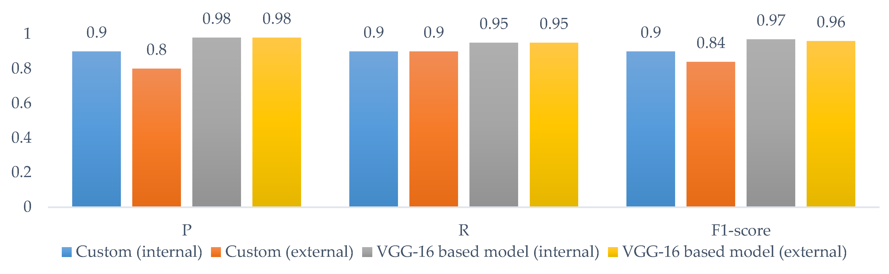
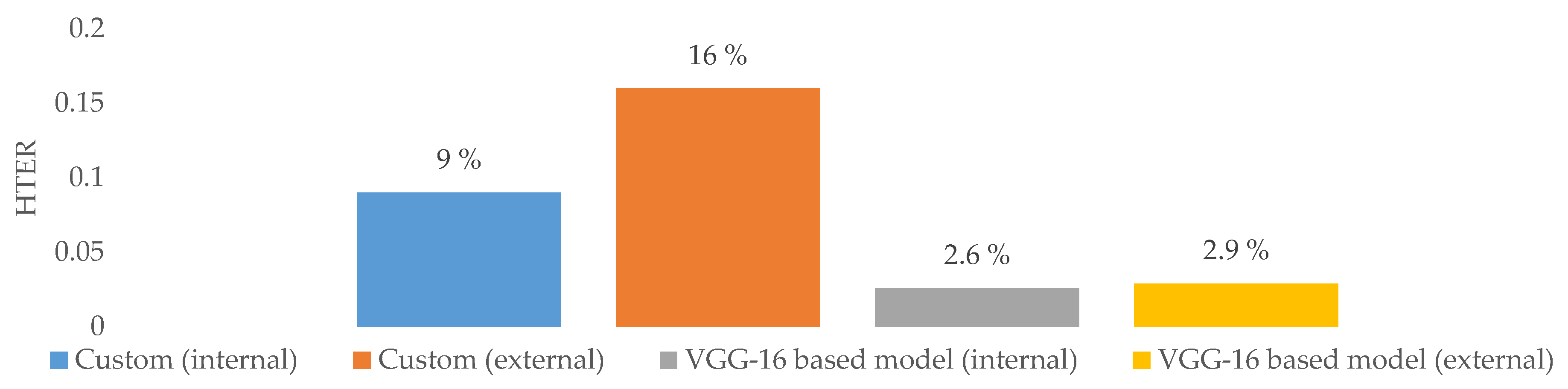
5.1. Performance of the Custom Model vs. the VGG-16-Based Model

The comparison of both models was made in terms of the following metrics: P, R and F1-score (Figure 9) and HTER (Figure 10). As shown in Figure 9, in the case of the custom model, its R value does not change between internal and external validation, whereas its P value decreases. This means that most of the colorized images are still classified as colorized in the external validation, but more original images are classified as colorized in the external validation. On the other hand, the VGG-16-based model has better results than the custom model, both for internal and external validation. In addition, for this model, the performance difference between internal validation is very small.
Additionally, as shown in Figure 10, the best results of HTER correspond to the VGG-16-based model for internal validation (2.6%), with a very close result for external validation (2.9%). In the case of the custom model, the HTER for internal validation is 9% and for external validation it is 16%. The VGG-16-based model not only has lower HTER values, but also less dispersion between its internal and external validation results.

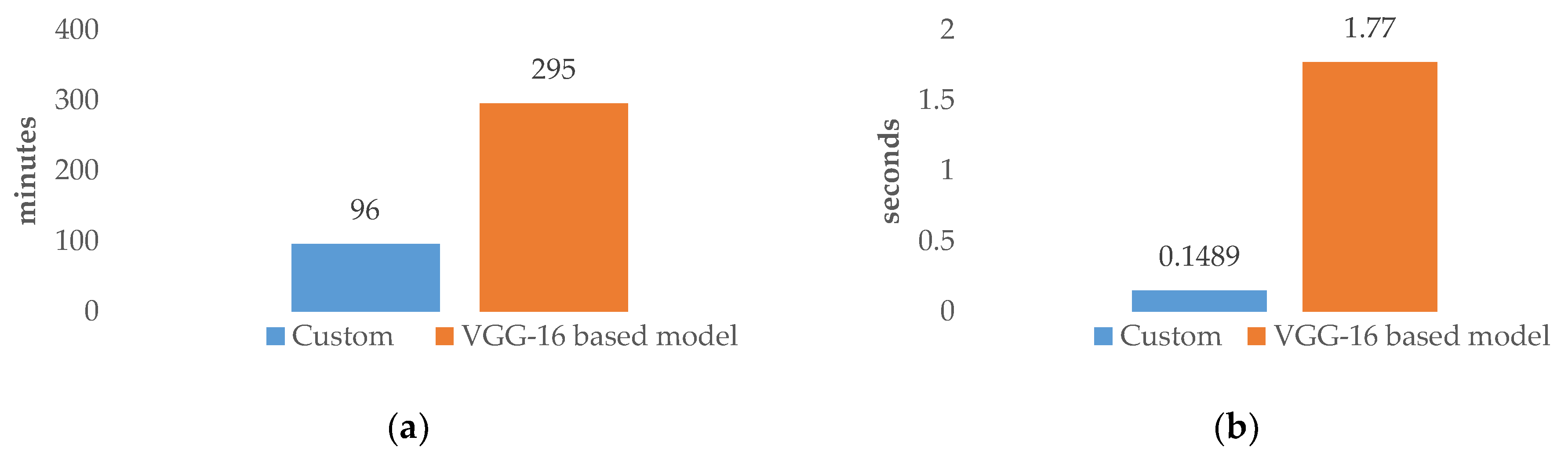
5.2. Inference Time of the Custom Model vs. the VGG-16-Based Model

An important aspect to consider when using trained models for large datasets is the inference time. In this criterion, models with shorter times are preferred. For this purpose, the training and inference times of the proposed models were compared. Figure 11a shows the training times (in minutes) and Figure 11b shows the inference times by image (in seconds). All tests were carried out using one of the GPUs (e.g., Nvidia K80, T4, P4 and P100) that Google Colaboratory provide for the users; in addition, Tensorflow was used. However, under this configuration the GPU is not selected by the user but by Google.
According to Figure 11, the VGG-16-based model takes about three times longer to train than the custom model. However, in terms of inference times, the fine-tuned model takes about twelve times longer than the custom model. The big difference between the inference times lies in the number of parameters of each one, while in the custom model it is 16 million, in the transfer-learning-based model it is 82 million. Therefore, the custom model is a good solution for high-volume image classification because it does not require a high-performance device.
In summary, the VGG-16-based model classifies the original and colorized images more accurately than the custom model (about +12% for F1-score) but requires longer training (×3) and inference times (×12).

5.3. Comparison with State-of-the-Art Works

Finally, the proposed models are compared with some state-of-the-art approaches. We focused on the ability of generalization, contrasting the results of internal validation with those of external validation.
In this regard, some recent approaches for colorizing detection using deep learning have emerged in the literature. For example, RecDeNet (Recolored Detection Network) uses three feature extraction blocks and a feature fusion module based on the CNNS. According to the reported results [25] (p.14), the internal accuracy is 87.4% and for external validation it is 76.7%. To converting accuracy into HTER, we assume that the confusion matrix has TN = TP and FN = FP, so that, for example, if acc = 87% with 100 true examples and 100 negative examples, then TN = TP = 87 and FN = FP = 13, providing an HTER of 13%. Therefore, for [25], we use an HTER of about 12.6% for internal validation and 22.3% for external validation.
As mentioned above, WISERNet reported HTER values of 0.95% for internal validation and 22.55% for external validation [14] (p.736). A modified WISERNet (referred to here as WISERNet II) also reports generalization problems, with an HTER of 0.89% for internal validation and 31.70% for external validation [15] (p.129). For progressive training using WISERNet (referred to here as WISERNet III), the reported HTER is reduced to 4.74% for external validation [26]. Table 4 shows the comparison results in terms of HTER for both internal and external validation.
It should be noted that not all works have used the same datasets. Therefore, the HTER values (internal or external) are only comparable within the works with the same datasets. For example, the best performance of the WISERNET networks has been provided by WiserNet III; while the best performance in our proposed networks corresponds to the VGG-16-based model. However, the HTER’s difference can be used to compare the results in Table 4, whose lowest value corresponds to our VGG-16-based model followed by WISERNet III. Therefore, the transfer-learning-based model outperforms the state-of-the-art approaches.

6. Conclusions and Future Work

This paper presented a custom model designed and trained to classify original and colorized images. The proposed architecture is not very deep and makes use of a parallelism block with two convolutional layers, followed by a convolutional layer and three fully connected layers. According to tests performed for the hyperparameter selection, it was found that the Adam and SGD optimizers allow similar classifier performance, but that the RMSProp optimizer is not recommended for this type of task. Additionally, it was found that the input image size significantly affects the performance of the classifier, so this hyperparameter related to the network structure should be considered in any experimental tests of classification models. Finally, we evaluated the impact of four dropout values for the penultimate layer of the network and found that there is no linear relationship between performance and dropout value, so this hyperparameter should also be included in the test protocols.
Additionally, we evaluated a model by transfer learning with the VGG-16 network, in which the pre-trained model was frozen down to the pooling_5 layer and only the fully-connected layers were modified and retrained. This model outperforms the custom model in terms of performance metrics, but it is 12x slower than the custom model. When these two models are compared with those existing in the state-of-the-art model, it is found that the proposed models are competitive in terms of generalization, improving on some of the results previously reported by other authors.
Therefore, in applications that require a very high classification rate such as in the forensic field, the transfer-learning-based model is an excellent choice. However, in real-time applications or for massive image classification, the custom model is the one that is recommended.
As future work we propose to evaluate other pre-trained models such as MobileNet, which could have shorter inference times than our VGG-16-based model.

Author Contributions

Formal analysis, D.M.B. and D.R.; Funding acquisition, D.M.B. and D.R.; Investigation, C.U.; Methodology, D.M.B. and D.R.; Software, C.U.; Writing—Original draft, C.U. and D.M.B.; Writing—Review and editing, D.R. All authors have read and agreed to the published version of the manuscript.

Funding

This research was funded by “Vicerrectoría de Investigaciones—Universidad Militar Nueva Granada”, grant number IMP-ING-2936.

Institutional Review Board Statement

Not applicable.

Informed Consent Statement

Not applicable.

Data Availability Statement

The data CG-1050 used in this study are openly available in [6].

Conflicts of Interest

The authors declare no conflict of interest.

References

  1. How Many Photos Will Be Taken in 2020? Available online: https://focus.mylio.com/tech-today/how-many-photos-will-be-taken-in-2020 (accessed on 17 December 2020).
  2. An, J.; Kpeyiton, K.G.; Shi, Q. Grayscale images colorization with convolutional neural networks. Soft Comput. 2020, 24, 4751–4758. [Google Scholar] [CrossRef]
  3. Cheng, Z.; Meng, F.; Mao, J. Semi-Auto Sketch Colorization Based on Conditional Generative Adversarial Networks. In Proceedings of the 12th International Congress on Image and Signal Processing, BioMedical Engineering and Informatics (CISP-BMEI), Suzhou, China, 19–21 October 2019. [Google Scholar] [CrossRef]
  4. Thakur, R.; Rohilla, R. Recent advances in digital image manipulation detection techniques: A brief review. Forensic Sci. Int. 2020, 312, 110311. [Google Scholar] [CrossRef] [PubMed]
  5. Castro, M.; Ballesteros, D.M.; Renza, D. A dataset of 1050-tampered color and grayscale images (CG-1050). Data Brief 2020, 28, 104864. [Google Scholar] [CrossRef] [PubMed]
  6. Castro, M.; Ballesteros, D.M.; Renza, D. CG-1050: Original and tampered images (Color and grayscale). Mendeley Data 2019. [Google Scholar] [CrossRef]
  7. Johari, M.M.; Behroozi, H. Context-Aware Colorization of Gray-Scale Images Utilizing a Cycle-Consistent Generative Adversarial Network Architecture. Neurocomputing 2020, 407, 94–104. [Google Scholar] [CrossRef]
  8. Fatima, A.; Hussain, W.; Rasool, S. Grey is the new RGB: How good is GAN-based image colorization for image compression? Multimed. Tools Appl. 2020. [Google Scholar] [CrossRef]
  9. Zhao, Y.; Po, L.M.; Cheung, K.W.; Yu, W.Y.; Rehman, Y.A.U. SCGAN: Saliency Map-guided Colorization with Generative Adversarial Network. IEEE Trans. Inf. Forensics Secur. 2020. [Google Scholar] [CrossRef]
  10. Ortiz, H.D.; Renza, D.; Ballesteros, D.M. Tampering detection on digital evidence for forensics purposes. Ing. Cienc. 2018, 14, 53–74. [Google Scholar] [CrossRef]
  11. Prasad, S.; Pal, A.K. A tamper detection suitable fragile watermarking scheme based on novel payload embedding strategy. Multimed. Tools Appl. 2020, 79, 1673–1705. [Google Scholar] [CrossRef]
  12. Bayar, B.; Stamm, M.C. A deep learning approach to universal image manipulation detection using a new convolutional layer. In Proceedings of the 4th ACM Workshop on Information Hiding and Multimedia Security, Vigo, Spain, 20–22 June 2016; pp. 5–10. [Google Scholar]
  13. Bayar, B.; Stamm, M.C. Constrained convolutional neural networks: A new approach towards general purpose image manipulation detection. IEEE Trans. Inf. Forensics Secur. 2018, 13, 2691–2706. [Google Scholar] [CrossRef]
  14. Zhuo, L.; Tan, S.; Zeng, J.; Lit, B. Fake colorized image detection with channel-wise convolution based deep-learning framework. In Proceedings of the 2018 Asia-Pacific Signal and Information Processing Association Annual Summit and Conference (APSIPA ASC), Honolulu, HI, USA, 12–15 November 2018; pp. 733–736. [Google Scholar] [CrossRef]
  15. Quan, W.; Wang, K.; Yan, D.M.; Pellerin, D.; Zhang, X. Impact of data preparation and CNN’s first layer on performance of image forensics: A case study of detecting colorized images. In Proceedings of the IEEE/WIC/ACM International Conference on Web Intelligence-Companion Volume, Thessaloniki, Greece, 14–17 October 2019; pp. 127–131. [Google Scholar] [CrossRef]
  16. Rao, Y.; Ni, J. A deep learning approach to detection of splicing and copy-move forgeries in images. In Proceedings of the 8th IEEE International Workshop on Information Forensics and Security (WIFS), Abu Dhabi, UAE, 4–7 December 2016; pp. 1–6. [Google Scholar] [CrossRef]
  17. Guo, Y.; Cao, X.; Zhang, W.; Wang, R. Fake colorized image detection. IEEE Trans. Inf. Forensics Secur. 2018, 13, 1932–1944. [Google Scholar] [CrossRef] [Green Version]
  18. Oostwal, E.; Straat, M.; Biehl, M. Hidden unit specialization in layered neural networks: ReLU vs. Sigmoidal activation. Physica A 2020, 564, 125517. [Google Scholar] [CrossRef]
  19. Simonyan, K.; Zisserman, A. Very deep convolutional networks for large-scale image recognition. In Proceedings of the 3rd International Conference on Learning Representations, ICLR 2015, San Diego, CA, USA, 7–9 May 2015; pp. 1–14. [Google Scholar]
  20. Results of ILSVRC. 2014. Available online: http://www.image-net.org/challenges/LSVRC/2014/results (accessed on 11 December 2020).
  21. Rangasamy, K.; As’ari, M.A.; Rahmad, N.A.; Ghazali, N.F. Hockey activity recognition using pre-trained deep learning model. ICT Express 2020, 6, 170–174. [Google Scholar] [CrossRef]
  22. Gupta, S.; Ullah, S.; Ahuja, K.; Tiwari, A.; Kumar, A. ALigN: A Highly Accurate Adaptive Layerwise Log_2_Lead Quantization of Pre-Trained Neural Networks. IEEE Access 2020, 8, 118899–118911. [Google Scholar] [CrossRef]
  23. Larsson, G.; Maire, M.; Shakhnarovich, G. Learning Representations for Automatic Colorization. In Lecture Notes in Computer Science; Leibe, B., Matas, J., Sebe, N., Welling, M., Eds.; Springer: Cham, Switzerland, 2016; Volume 9908. [Google Scholar] [CrossRef] [Green Version]
  24. Soydaner, D. A Comparison of Optimization Algorithms for Deep Learning. Int. J. Pattern Recognit. Artif. Intell. 2020, 34, 2052013. [Google Scholar] [CrossRef]
  25. Yan, Y.; Ren, W.; Cao, X. Recolored Image Detection via a Deep Discriminative Model. IEEE Trans. Inf. Forensics Secur. 2019, 14, 5–17. [Google Scholar] [CrossRef]
  26. Quan, W.; Wang, K.; Yan, D.M.; Pellerin, D.; Zhang, X. Improving the Generalization of Colorized Image Detection with Enhanced Training of CNN. In Proceedings of the 11th International Symposium on Image and Signal Processing and Analysis (ISPA), Dubrovnik, Croatia, 23–25 September 2019; pp. 246–252. [Google Scholar] [CrossRef]
  27. Iizuka, S.; Simo-Serra, E.; Ishikawa, H. Let there be color! Joint end-to-end learning of global and local image priors for automatic image colorization with simultaneous classification. ACM Trans. Graph. 2016, 35, 1–11. [Google Scholar] [CrossRef]
  28. Zhang, R.; Isola, P.; Efros, A.A. Colorful Image Colorization. In Lect. Notes Comput. Sci.; Leibe, B., Matas, J., Sebe, N., Welling, M., Eds.; Springer: Cham, Switzerland, 2016; Volume 9907. [Google Scholar] [CrossRef] [Green Version]
Figure 1. Example of manual colorization through Photoshop software: (a) original grayscale image; (b) colorized image corresponding to the girl’s dress. Source: CG-1050 dataset [5,6].
Applsci 11 00476 g001
Figure 2. The proposed architecture. Conv is convolutional layer; BatchN is batch normalization; MaxPool is max-pooling; FC is the fully-connected layer.
Applsci 11 00476 g002
Figure 3. VGG-16 architecture. Conv means convolutional layer; and FC means fully-connected layer.
Applsci 11 00476 g003
Figure 4. F1-scores using different datasets: (a) custom model using DA; (b) custom model using DB; (c) custom model using DC; (d) VGG-16 based model using DA; (e) VGG-16-based model using DB; (f) VGG-16-based model using DC.
Applsci 11 00476 g004
Figure 5. Impact of the input image size in the custom model in terms of HTER (the lower the better).
Applsci 11 00476 g005
Figure 6. Impact of the dropout value in the custom model in terms of HTER (the lower the better).
Applsci 11 00476 g006
Figure 7. Impact of the optimizer in the custom model in terms of HTER (the lower the better).
Applsci 11 00476 g007
Figure 8. Impact of the optimizer in the transfer-learning-based model in terms of HTER (the lower the better).
Applsci 11 00476 g008
Figure 9. Performance evaluation of the custom model and the transfer-learning-based model: P, R, and F1-score (the higher the better).
Applsci 11 00476 g009
Figure 10. Performance evaluation of the custom model and transfer-learning-based model: HTER (the lower the better).
Applsci 11 00476 g010
Figure 11. Time comparison between the custom model and transfer-learning-based model: (a) training time; (b) inference time.
Applsci 11 00476 g011
Table 1. Summary of the proposed custom architecture for the classification of colorized images.
LayerNo. of FiltersKernel SizeStride
Conv2D-A64(1,1)1
BatchN-A---------------------------
MaxPool-A---------(3,3)2
Conv2D-B32(3,3)1
BatchN-B---------------------------
MaxPool-B---------(3,3)2
Conv2D-C64(1,1)1
BatchN-C---------------------------
MaxPool-C---------(3,3)2
Conv2D-D32(3,3)1
BatchN-D---------------------------
MaxPool-D---------(3,3)2
Conv2D-E64(5,5)2
MaxPool-E---------(5,5)2
FC-A400------------------
FC-B200------------------
FC-C2------------------
Table 2. General characteristics of the three data sets used (DA, DB, DC).
DatasetColorization TypeNumber of Images (Original vs. Colorized)
DAmanual331 vs. 331
DBmanual and automatic4719 vs. 4719
DCmanual and automatic9506 vs. 9506
Table 3. Experimental hyperparameters evaluated for the proposed custom network.
HyperparameterOptions
Image size256 × 256, 400 × 400, 512 × 512
Dropout0.15, 0.25, 0.35, 0.45
OptimizerRMSProp, SGD, Adam
Table 4. Comparison of the proposed models with representative methods of the state-of-the-art approaches in terms of HTER (the lower the better).
MethodDatasetHTER
(Internal Validation)
HTER
(External Validation)
HTER’s Difference
RecDeNet [25]PASCAL 201212.622.3+9.7
WISERNet I [14][23] + [27] + [28]0.9522.5+21.55
WISERNet II [15][23] + [27] + [28]0.8931.7+30.81
WISERNet III [26][23] + [27] + [28]0.894.7+3.81
Custom model[5] + [23]9.0016.0+7
VGG-16-based model[5] + [23]2.602.9+0.3
Publisher’s Note: MDPI stays neutral with regard to jurisdictional claims in published maps and institutional affiliations.

