ALARP Criteria to Estimate Acceptability and Tolerability Thresholds of the Investment Risk

Abstract

Assessing the riskiness of investments in civil works is an integral part of the decision-making process. The main limitation is the absence, both in the regulatory landscape and in the literature of the sector, of threshold values that can guide the analyst in expressing an assessment on the acceptance of the investment risk. The aim of the paper is to define a risk management model that overcomes this gap by introducing acceptability and tolerability thresholds for project risk. The idea is to jointly use: (i) the As Low As Reasonably Practicable (ALARP) logic, from which the concepts threshold of acceptability and tolerability of risk derive, for the first time applied to assess the project risk in the civil field; (ii) the Capital Asset Pricing Model (CAPM) and statistical methods to define an innovative methodology for estimating the aforementioned threshold values. According to the proposed approach, these risk limit values can be specified according to both the investment sector and the socio-economic context of the project. The implementation of the methodology in the civil company sector in Europe allows to validate the described model. The elaborations show that the financial performance of the project is widely acceptable if the Expected Internal Rate of Return is greater than 7.8%; unacceptable if the expected rate of return is less than 5.6%; and tolerable as an ALARP if the expected rate is between 5.6% and 7.8%. The estimated acceptability and tolerability thresholds can provide the economic operator with a more immediate and consistent evaluation of the triangular balance of risks, costs, and benefits. This allows the decision-making process to become more rational and transparent.

1. Introduction

There are many definitions of risk in the literature. According to the Society of Risk Analysis [1], risk is «the potential realization of unwanted and negative consequences arising from an event». By ISO 31000 [2] standards, risk is referred to the «possibility of an effect». The UK Cabinet Office [3] brings risk back to the “uncertainty of outcome”. Regarding the systematic terminology of the sector, there are variations in relation both to the scientific sector and according to the needs and goals to be achieved [4]. Instead, what is generally recognized is the centrality of risk whenever it is necessary to solve a problem or plan [5]. In fact, numerous international bodies and organizations have promulgated regulatory guidelines about risk management.

ISO 31000 [6] has defined guidelines and principles useful to harmonize the management processes of any risk in both existing and future standards. Similarly, the International Atomic Energy Agency (IAEA) [7], the European Commission (EC) [8], the Health Safety and Executive (HSE) [9] and the World Health Organization (WHO) [10] have defined etymological aspects, standards, and procedures for safeguarding human life in high-risk sectors.

In this paper, the focus is on the ex-ante assessment of the risk that characterizes investments in the civil sector. Also in this sector, the European legislative framework acknowledges the key role that risk analysis must play in the economic evaluation of projects. The Guide to the Cost-Benefit Analysis of the European Commission (EC) for the 2014–2020 programming period identifies the following four essential phases to assess the investment risk: 1. sensitivity analysis; 2. qualitative risk analysis; 3. probabilistic risk analysis; 4. possible definition of prevention and/or mitigation actions [11]. EC Regulation 1303/2013 clarifies that risk analysis is needed in situations where the exposure to residual risk, i.e., the risk that remains despite the mitigation strategies undertaken, is substantial. However, it can also be performed because of the dimension of the project or in relation to the accessibility of the data required for the evaluation. On the other hand, there is no guideline giving information on acceptable levels of investment risk [12].

To fill this gap, an innovative protocol is proposed for assessing the acceptability of the investment risk of civil works. The idea is to bring ALARP (As Low As Reasonably Practicable) logic into the procedural frameworks of Cost-Benefit Analysis (CBA). Widely used in the field of security, ALARP logic gives a guide to accepting the risk of loss of life in high-risk sectors (energy, nuclear, oil and gas). According to this approach, a risk is ALARP if it is between the thresholds of acceptability and thresholds of tolerability, or if the costs of reducing it are not disproportionately high in relation to the benefits obtainable [9].

From the ALARP approach, criteria relating to risk acceptability and tolerability thresholds are borrowed, becoming useful in assessing the risk acceptability of the project. In particularly, it was considered that the ALARP principle could represent a general way of thinking whenever the overall goal is a triangular balancing of costs, benefits, and risks. The main novelty of the model concerns the methodology to assess these threshold values. This methodology is based on the joint use of the Capital Asset Pricing Model (CAPM) and statistical tools to estimate the acceptance limit values to both the investment sector and the socio-economic context of the investment project.

If regulatory guidelines and sector literature provide indications for estimating investment risk, there are no specific references for stable within which range this risk can be considered acceptable for the investor. In this sense, by introducing the ALAPR logic in the CBA procedural scheme, we provide objective criteria to establish whether the probability of investment failure is unacceptable, ALARP, or widely acceptable for the economic operator.

Specifically, by comparing the Expected Internal Rate of Return E(IRR) of the investment with the two thresholds of acceptability and tolerability defined, the analyst can express a consistent and objective judgement on the financial performance of the project under risk conditions. More in detail, the introduction of acceptability and tolerability thresholds can represent a useful guide to be able to provide a judgment on the economic performance of an investment in the civil field, when the result of the analysis is expressed in stochastic terms.

The defined risk management model thus shows the importance of providing in guidelines and regulations, not only methods for estimating the probability of investment failure, but also useful approaches for assessing the acceptability of risk based on threshold values.

The paper is structured in five sections. Section 2 analyses criteria and techniques for risk assessment in the safety field and for the analysis of the investment risk in civil works. Section 3 defines the model for assessing the project risk, with particular attention to the methodology for estimating the acceptance threshold values. In Section 4, the acceptability and tolerability thresholds of the investment risk for civil sector projects in Europe are estimated. The last section shows the results of the study, and possible research perspectives.

2. Theoretical Basis about Risk

To characterize the investment risk assessment model, it is necessary to define: (1) the main phases in which a general risk management process is structured; (2) the As Low As Reasonably Practicable risk acceptability criterion; (3) the investment risk analysis techniques generally used in practice. This is in order both to define in which phase of the risk management process the ALARP principle can intervene, and to verify the applicability of the ALARP criterion to the Cost-Benefit Analysis of civil engineering projects.

2.1. Risk Management Principles

Aim of risk management is to ensure that people, environment, and resources are protected from harmful consequences resulting from human activities or natural events. In other words, risk management makes it possible to plan strategies that are useful to contain hazards/threats of an activity or to reduce their potential damage [13].

There are three strategies generally used to manage the risk: risk-informed, cautionary/precautionary, and discursive. The first refers to the planning of mitigation interventions deriving from the timely qualitative, quantitative, or semi-quantitative assessment of risky assets. The second is also defined as a resilience strategy and consists of risk containment, monitoring, and screening actions. The third one, on the other hand, is based on actions aimed at reducing uncertainties, explaining the evolutionary dynamics of risky processes, or involving people affected by risky activities [14].

Therefore, Risk Management is the set of processes that are useful for identifying, analysing, quantifying, eliminating, and monitoring the associated risks with the performance of any activity and it consists of the logical-operational phases described below [2,6,15,16,17].

The first step is to establish the context or to define the scope and objectives to be pursued, considering both the costs and benefits deriving from risk management.

The second step of risk assessment comprises: (2.1) identification, (2.2) analysis, and (2.3) assessment of risks. Sub-step (2.1) is used to recognize potential dangers and threats that prevent the achievement of the objectives defined in the previous step (establish context). (2.2) is useful for understanding the nature of risky events as well as for determining the causes and consequences deriving from them. In (2.3), the information gathered from the identification and analysis phases is useful to establish whether the risk is acceptable or whether it is necessary to undertake mitigation strategies. In this phase, each identified risk is given a “weight” to draw up a list of priorities useful to guide the subsequent step of risk treatment. Weighting means estimating the level of risk according to the probability of occurrence of the event and its consequences.

The following phase is the risk treatment, which includes: (3.1) the selection of the mitigation measures; (3.2) the implementation of the prepared plan; (3.3) the analysis and assessment of residual risk, i.e., the risk that remains despite the mitigation strategy undertaken. Mitigation strategies can be about retention actions, if the risk cannot be reduced, avoided or transferred; avoidance actions, if the source of risk is eliminated or the activity is interrupted; transfer actions, if the risk is transferred to another asset; control actions, if you act on the probability of occurrence of the event or its consequences on one of the two terms or both; acceptance actions, when there is no possible and/or sustainable mitigation intervention for which the risk is accepted as it is presented.

Communication and Consultation and Monitoring and Review are also essential, but they are continuous processes that accompany all the phases of Risk Management [18,19]

Figure 1 summarizes the Risk Management Process (RMP) phases.

2.2. ALARP Risk Evaluation Criteria

Risk assessment is widely adopted in the safety field where it is necessary to safeguard human life from the consequences of dangerous activity performance. In this sector, risk management was traditionally based on a prescriptive regulation regime, in which the requirements for the design and operation of plants were specified in detail. Over time, there has been a gradual shift towards goal-oriented regimes that place more emphasis on the target to be achieved rather than the means to do so. This has led to integrated risk governance approaches that generate higher levels of performance in terms of both productivity and risk reduction [7,8,9,10].

In these approaches, the Quantitative Risk Assessment (QRA) is increasingly used, so much so that many regulatory agencies impose quantitative methods that can improve the economic efficiency of the decision-making related to risk management [20,21]. Consider, for instance, the guidelines of ERM-Hong Kong Ltd. [22] for the management of landslide risk and the regulation of the Association of Professional Engineers and Geoscientists of British Columbia (APEGBC) [23] who also considers the application of quantitative assessments for land use planning.

However, when riskiness is assessed in terms of the probability of loss of human life, it becomes complex to establish acceptable levels of risk as it is necessary to include in the assessment not only ethical, social, and legal issues but also political and economic ones [24,25,26]. For this reason, decision makers and political actors often resort to quantitative methods together with useful criteria to evaluate the tolerability/acceptability of the risk. In 1992, the British agency of the Health and Safety Executive (HSE), to manage the inherent hazard of industrial processes, defined some general principles of risk acceptance [27]:

• The accountability principle. The definition of risk acceptance criteria must be clear and transparent, based on quantitative definitions and objective assessments;
• The principle of equivalency. The risk must be compared with limit thresholds that derive from the analysis of similar activities or similar systems to that to be assessed and who are widely recognized as acceptable or tolerable;
• The holistic principle. Security decisions must be based on a holistic view of all risks. Only when the overall risk of the activity itself has been examined, can mitigation measures be proposed;
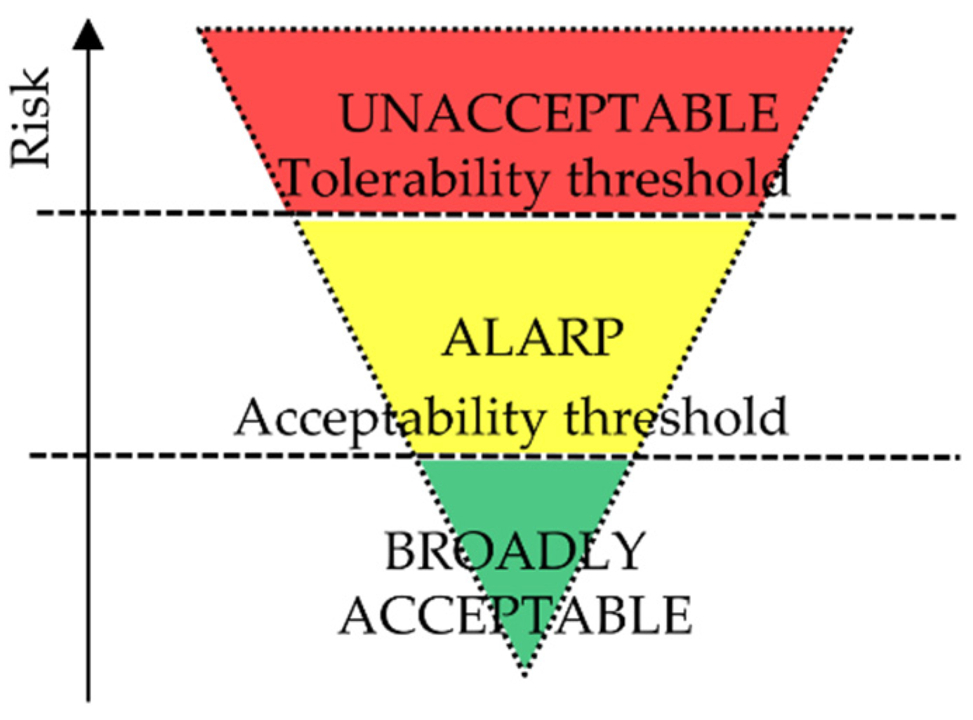
• The ALARP Principle. Risks must be reduced to be As Low As Reasonably Practicable. In other words, all mitigation measures must be implemented until the costs appear disproportionate to the achievable benefits. In the ALARP context, threshold values are defined for “acceptable” risks and “tolerable” risks.

According to ALARP principle, risks that fall below the tolerance threshold must be necessarily reduced because they are unacceptable. Risks included between the tolerability and acceptability thresholds are in the ALARP area, so it is necessary to mitigate them until they are reasonably practicable. Finally, risks above the acceptability threshold are “widely acceptable”, so there is no need to mitigate them.

The ALARP criteria, generally applied in the high-risk areas of industrial engineering, requires those responsible for the activity to reduce risks to levels that are ‘As Low as Reasonably Practicable’ [28]. As such, the principle implies an effective recognition that while in most circumstances risk can be reduced, beyond a certain point further risk reduction is always more costly to implement.

Figure 2 shows the ALARP principle.

The reference literature also distinguishes individual risk from social risk.

The former is defined as the “frequency at which an individual is expected to be subjected to a certain level of harm as a result of an accident in a major risk industry”. In other words, it can be defined as the risk of death to which a single individual is subjected in an unsafe place at a given moment in time. This risk gives an annual probability of death value for a certain position.

The social risk, on the other hand, is given by the frequency with which a certain number of people are subjected to a certain level of damage following a specific accidental event.

This risk is well illustrated by the F–N curve, which correlates the number of deaths (N) on the horizontal axis with the frequency (F) of one or more deaths on the vertical axis. These curves were developed originally to assess nuclear risks since tolerance thresholds, which reflected the social aversion to more deaths during a single catastrophic event.

In these charts, the two thresholds of risk acceptability and tolerability are a function of such parameters as slope and anchor point. A first indication of the development of the social risk curves is given by the historical accident curves in each region, which are important indications of the starting point and the slope to be associated with the limit lines. The former parameter, the anchor point, is the cumulative limit frequency (F) for a certain number of fatalities. The inclination, on the other hand, which is always negative and generally ranges between −1 and −2, is a function of risk aversion towards accidents with a progressively increasing number of fatalities [27,28,29].

Figure 3 shows a generic F-N graph, divided into four areas. In the unacceptable region, the risk should be reduced regardless of the investment. It follows that if an investment is unsustainable, exposed people should be turned away. In the intense security region, the probability of the catastrophic event occurring is very low but must always be kept under control. In the widely acceptable region, no investment is needed to further reduce risk. Finally, in the tolerable region, risk should be further reduced if the ALARP principle is practicable, that is cost-benefit approaches are used to evaluate the convenience of a mitigation option or to compare the various possible interventions.

In other terms, the costs of implementing risk reduction measures are compared with the reduced risks assessed in monetary terms, thus assigning an economic value to life. In literature, there are several estimates of the economic value of life in which people are considered as a resource in economic activities. However, the ethical criticisms to this approach are equally relevant. Thus, cost effectiveness analysis is often used to avoid attributing a cost to human life [30]. According to this method, the ratio between the cost of the risk reduction measures and the risk reduction itself is assessed, avoiding giving life an economic value. In this case, indicators such as gross-cost-of-averting-a-fatality (GCAF) and net-cost-of-averting-a-fatality (NCAF) are estimated:

$$\mathrm{GCAF}=\frac{\Delta \mathrm{C}}{\Delta \mathrm{R}},$$

(1)

$$\mathrm{NCAF}=\frac{\Delta \mathrm{C} - \Delta \mathrm{B}}{\Delta \mathrm{R}},$$

(2)

where ΔC is the cost of the risk mitigation intervention; ΔB is the benefits of implementing the mitigation strategy; ΔR is the risk reduction arising from the planned intervention, in terms of victims or damage avoided.

To understand the dynamism and applicability of the ALARP approach, it is increasingly used for land-use planning in the immediate vicinity of industries or dams, for landslide risk management as well as for risk assessment in tunnels [31,32].

According to Baybutt [33], the ALARP principle provides a useful framework for establishing risk tolerance criteria. Abrahamsen et al. [34] argue that the ALARP principle should be interpreted dynamically. Again, Redmill [35] believes that the ALARP criterion can represent “a general thinking way”. Therefore, it can also find original application in the risk assessment of investments in the civil field, where the main objective is always a triangular balance between mitigation costs, achievable benefits, and risk containment. In this case, the critical aspect concerns the estimation of the threshold values of acceptability and tolerability useful to define the region where the investment risk for the economic operator is reasonably feasible since it is ALARP.

2.3. The Risk Management Process Referred to the Economic Evaluation of Projects

Risk Management is well integrated with decision theory. On the topic, Althaus, Bridgman and Davis [36] and Aven [24] highlight not only that the phases of the decision-making process are in line with those of the risk analysis process, but also that the risk field provides multiple inputs that are useful to support analysts during decision phase, among others: the conceptualization and characterization of the problem in terms of goals, criteria, risks, uncertainty, knowledge and priorities; the hierarchization of the problem in order to understand its key principles; the analysis of statistical data to identify the elements of risk; risk assessment, including quantitative, of potential alternatives; and the perception of risk by the various actors involved in the decision-making process.

So, risk management becomes critical when it is necessary to express a judgment of economic convenience on investments. This is particularly true when the uncertainty concerning sensitive project variables makes it difficult to express the outcome of the Cost Benefit Analysis (CBA) in deterministic terms, as in the case of major interventions or when the data needed for the analysis is incomplete or difficult to find [11]. This leads the evaluator to conduct the analysis in stochastic terms. In this case, it is needed to:

• Identify the sensitive variables of the system, i.e., those that have a significant influence on the final value of the economic performance indicator. According to the European Commission’s Guide to Cost-Benefit Analysis, “critical” variables are considered to be those for which a change of ±1% in the estimated value results in a variation of more than ±1% of the Net Present Value (NPV) [11];
• Describe the sensitive variables in stochastic terms, that is, derive the probability distribution of the risky parameters of the analysis, identified in point (1);
• Estimate the probability distributions of the investment performance indicators. This step returns the stochastic description of the profitability indicator as a function of the probability distribution associated with the risky parameters in point (2). If we consider the Internal Rate of Return (IRR) as an indicator of economic performance, then:

$${\displaystyle \sum }_{t=0}^n\frac{B_t-C_t}{{\left(1+IRR\right)}^t}=0,$$

(3)

where:

−

B_t are the benefits at time t and are a function of both probabilistic $\left(B_{p1}, \dots B_{pn}\right)$ and deterministic $\left(B_{d1}, \dots B_{dn}\right)$ terms;

−

C_t represent the costs at time t described in both probabilistic $\left(C_{p1}, \dots C_{pn}\right)$ and deterministic $\left(C_{d1}, \dots ,C_{dn}\right)$ terms;

−

IRR is the Expected Internal Rate of Return.

In fact, it is by analyzing the IRR probability density function and the cumulative probability distribution of the IRR that it is possible to derive important information on the riskiness of the project [37].

From the punctual probability distribution of the profitability indicator—shown in Figure 4a—it is possible to read all the possible values of the indicator and the probability of each of them occurring. For this reason, the expected value or mean value of the variable is also derived from this distribution.

Let the IRR be a continuous random variable with probability density f(_IRR), the expected value (mean value or mathematical hope) of the variable IRR is defined as the integral extended in all ℝ of the product between IRR and the density function f(_IRR):

$$\mathrm{E}\left(\mathrm{IRR}\right)={{\displaystyle \int }}_{-\infty }^{+\infty }\mathrm{IRR}· f\left(\mathrm{IRR}\right).$$

(4)

If we discretize the probability density function of IRR, then the expected value of the discrete random variable IRR is the sum of the products between IRR_i values and the respective probability $\mathrm{f}$(_IRRi):

$$\mathrm{E}\left(\mathrm{IRR}\right)={\sum }_{\mathrm{i}=1}^{\mathrm{n}}{\mathrm{IRR}}_{\mathrm{i}}·f \left({\mathrm{IRR}}_i\right).$$

(5)

In (5), n means the number of discretization intervals of the probability distribution related to the random variable IRR.

The cumulative probability curve F_(IRR), schematized in Figure 4b, also provides relevant information on the risk of the project. In fact, it allows to verify what is the probability of having an IRR higher or lower than a value considered critical.

There are many studies in the literature that provide approaches to estimate the probability of project failure with reference to different investment sectors.

Cheah and Liu evaluated the governmental support in infrastructure projects as real options using Monte Carlo simulation [38].

Platon and Constantinescu [39] highlighted how the stochastic method can be widely applied in the economic evaluation of investments due to the advantages recognized by both practitioners and the academic community.

Again, Arnold and Özgür [40] addressed the problem of estimating the economic risk of decentralized renewable energy infrastructures by considering the entire life cycle of the projects under analysis.

Lei et al. [41] proposed a methodology that integrates probabilistic analysis and multi-objective programming to assess the sustainability of Chinese wind energy projects investment sectors.

The sector literature shows a wide application of probabilistic methods to assess the economic risk of the project. On the other hand, there is a lack of objective criteria for determining whether the risk and residual risk are acceptable to the investor. Thus, the next paragraph characterizes an innovative investment risk assessment model and shows how this criticality can be overcome by resorting to the ALARP principle and to the concepts of acceptability threshold and risk tolerability threshold. Figure 5 summarizes the three main steps of the risk analysis.

3. ALARP and CAPM. A Model for the Investment Risk Management

The aim of this paper is to characterize a model for assessing the acceptability of investment risk for civil works in the case of ex-ante financial analysis. In order to do so, it is necessary firstly: (1) to set objective criteria to assess the acceptability of investment risk; and (2) to establish a methodology to estimate the acceptance limit values. To solve point 1, we indicate to the As Low As Reasonably Practicable (ALARP) logic. According to this principle, risk assessment is related to two thresholds: the threshold of acceptability and the threshold of tolerability. Specifically, a risk is: (i) ALARP if it is between these two thresholds, i.e., if the costs of risk mitigation are not disproportionate to the benefits to be obtained; (ii) intolerable if it is above the tolerability threshold; and (iii) is broadly acceptable if it falls below the acceptability threshold [42,43,44]. A further crucial step is phase 2. This concerns the definition of a methodology for the estimation of acceptable and tolerable project risk thresholds. The novelty consists in the joint use of the Capital Asset Pricing Model (CAPM) and statistical survey tools, thus making it possible to assess the risk thresholds according to both the socio-economic reference context of the project and the investment sector.

This section on the characterization of the assessment model is divided into two Sub-Sections: Section 3.1 describes the steps of the risk assessment protocol; Section 3.2 details the methodology for estimating risk acceptance thresholds.

3.1. Phases of the Risk Assessment Model

The investment risk management model follows the logical and operational steps of the risk management process described in Figure 1.

Step 1: Establish the context. In this first phase, it is first required to establish the objective that the financial operator intends to achieve, i.e., to prevent the investment failure. Therefore, the costs and benefits of the project are estimated, the analysis period is determined and the return on investment is assessed, using financial performance indicators such as Net Present Value (NPV), Internal Rate of Return (IRR), Payback Period, and Benefit-Cost ratio.

Step 2: Risk assessment. This phase consists of the following three steps: identification of risk variables; risk analysis; risk estimation.

−

Step 2.1. Identification of risk variables. This can be done by applying sensitivity analysis, which enables the identification of those project variables whose variations (positive or negative) have the greatest impact on the financial performance of the initiative.

−

Step 2.2. Risk analysis, first qualitative then quantitative. The qualitative risk analysis comprises a list of the adverse events to which the project is vulnerable and the resulting definition of the risk matrix. From this matrix it is then possible to interpret, for each adverse event, the relative level of risk based on the probability of occurrence and the severity of the impact.

The quantitative risk analysis requires first the attribution of the probability distribution for each risk variable. This distribution can be derived from experimental data, similar cases in the literature or expert consultations. Implementing Monte Carlo analysis, using specific software, we then derive the probability density function and the cumulative probability distribution of the financial performance indicator. The former provides the expected or average value of the indicator, while the cumulative probability distribution shows the probability of having an IRR above or below a certain critical value.

−

Step 2.3. Risk estimation, in which the acceptability of the investment risk is verified. In this phase, the concepts of risk acceptability threshold and risk tolerability threshold derived from ALARP logic are applied. So, here we find the main novelty of the model.

The tolerability threshold separates the region of unacceptable risk from the region where the risk is tolerable as ALARP. We therefore assume that an investment whose return is equal to the return expected from a project with an average risk profile, i.e., one that is on average representative of civil enterprises of a given socio-economic context, is tolerable.

The acceptability threshold, on the other hand, separates the ALARP risk region from the region in which the risk is broadly acceptable to the investor. Since the expected return of the project increases as the investment risk rises, we assume that an investment whose average return is at least equal to the return expected from a project with a high-risk profile, i.e., representative of first-quartile civil enterprises—namely those with the lowest returns and consequently the riskiest of a given territorial context—is acceptable to the economic operator.

Having conceptually defined the thresholds of acceptability and tolerability, it is possible to assess the riskiness of the project in terms of expected IRR, starting from the probability density function of the profitability index.

As shown in Figure 6, we have that:

−

The project initiative is widely acceptable to the investor if E(IRR) > r_a, i.e., if the expected IRR of the project is higher than the return expected from a project with an average risk profile. In this case, no risk mitigation measures need to be defined in order to increase the project return (Figure 6a);

−

The project initiative is unacceptable to the investor if E(IRR) < r_t or if the expected IRR of the project is lower than the return expected from a project with a high-risk profile. In this case, the project is unsustainable, so that it is necessary to define improvement measures which decrease the risk of failure or increase the profitability of the initiative (Figure 6b);

−

The project initiative has a tolerable risk, if r_a < E(IRR) < r_t, i.e., if the expected IRR of the project is between the return expected from a project with a medium-risk profile and the return expected from a project with a high-risk profile. In this case, mitigation measures should be implemented that do not have disproportionate costs compared to the achievable benefits (Figure 6c).

Step 3: risk treatment. If the risk is unacceptable or tolerable for the investor (Figure 6b,c), it is first necessary to define changes to the project, then to assess the residual risk, i.e., the risk which remains despite the containment strategy undertaken. Then, the riskiness of the project is evaluated again in terms of expected IRR (Figure 6).

Specifically, consider that the pre-mitigation intervention is in a tolerable condition (represented in Figure 6c). In this case, the following scenarios may occur:

−

The post mitigation design initiative is in a condition of broad acceptability (Figure 6a). The mitigation measures should be implemented;

−

The post mitigation project initiative is in an unacceptable or ALARP condition for the investor (Figure 6b,c). The pre-mitigation project is tolerable according to the ALARP principle, i.e., it has been shown that the improvement measures have disproportionate costs compared to the achievable benefits.

Consider, on the other hand, the case where the pre-mitigation intervention is in an unacceptable condition (Figure 6b). It may be that:

−

The post mitigation design initiative is in a condition of broad acceptability (Figure 6a). The mitigation measures should be applied;

−

The design initiative after mitigation still falls into an unacceptable condition (Figure 6b). The project is still risky, and the planned interventions cannot be realized;

−

The project initiative after mitigation is in a tolerable condition (Figure 6c). The investment risk is now tolerable according to the ALARP principle, i.e., if any other improvement intervention does not result in greater benefits at lower costs.

It is important to underline that the planning of risk mitigation measures is a crucial step in the analysis model and thus on the outcome of the assessment [45].

Risk mitigation strategies may take the form of structural modifications or changes in the economic and financial management of the project. This entails different costs from those estimated by the initial scenario, as well as different revenues. These changes may also significantly influence the profitability index of the intervention and therefore the value of the Expected Internal Rate of Return. In other words, the implementation of mitigation strategies can lead to a distancing/approaching of the E(IRR) from the thresholds of acceptability and tolerability of the risk. Therefore, in order to prevent the project from failing, it is absolutely necessary that the investor assesses ex-ante all possible mitigation measures to determine the optimal balance between cost reduction, revenue increase, and residual risk containment.

To compare two or more mitigation strategies, the risk assessment described above can be combined with the estimation of the net-cost-of-preventing-a-failure (NPAF):

$$\mathrm{NPAF}=\frac{\Delta \mathrm{C}}{\Delta \mathrm{R}},$$

(6)

where: ΔC is the cost of the risk mitigation intervention net of benefits; ΔR is the reduction of risk resulting from the implementation of the planned intervention. ΔR is given by the difference between the E(IRR) before mitigation and the cumulative probability of E(IRR) after mitigation. It is evident that once a maximum cost is set that the investor is willing to bear to make the project initiative widely acceptable—the higher the ΔR, the better the planned mitigation strategy performs.

3.2. A Statistical Methodology for the Estimation of the Tolerability and Acceptability Thresholds of the Investment Risk

Estimating investment risk thresholds is essential for the characterization of the model described in the previous paragraph. The objective is to define a methodology for establishing the minimum tolerable return and the minimum acceptable return for the investor. These returns depend on factors such as: the investment sector of the project; the risk appetite of the financing party; and the specific socio-economic conditions of the area in which the intervention is located.

Thus, the theoretical reference to establish these limit values is the Capital Asset Pricing Model, as it allows the assessment of the risk-adjusted discount rate r(β), which can be interpreted as the minimum return expected from an investment project with a risk profile β [46].

In order to define the meaning of the minimum tolerable return r_t and the minimum acceptable return r_a for the investor on which the model is based, it is necessary to briefly recall the theoretical framework of the CAPM.

The Capital Asset Pricing Model was introduced into financial economics by Sharpe [47] and Lintner [48] to explain how the risk of a financial investment affects its expected return. It is an extension of the market portfolio model proposed by Markowitz [49], also known as the mean-variance model, according to which investors are risk-averse and will therefore select a trading-off portfolio between risk and return for a certain investment period [50]. This means that investors will choose efficient portfolios that minimize the variance of the portfolio return for a specific level of expected return, or maximize the expected return, given the specific level of variance. The CAPM assumptions are specified below. They are the same as in the Markowitz portfolio model, plus assumptions 2 and 3 added by Sharpe [47] and Lintner [48]:

(1)

All investors select efficient portfolios to maximize the utility of their investments. In other words, investors are risk-averse, so they maximize utility and focus only on their return (mean) and relative risk (variance);

(2)

Investors can borrow or lend funds at the risk-free rate of return;

(3)

All investors have homogeneous expectations, which means that they estimate the same distributions for future rates of return;

(4)

All investors hold investments for the same period of time;

(5)

Investors are able to buy or sell shares in any security or portfolio they hold;

(6)

There are no taxes or transaction costs on the purchase or sale of assets;

(7)

There is no inflation or any change in interest rates;

(8)

Capital markets are in equilibrium, and all investments are fairly priced, i.e., investors cannot influence prices [51].

The CAPM equation in accordance with the assumptions of Sharpe and Lintner can be expressed as follows:

E(r_i) = r_f + β · [E(r_m) − r_f],

(7)

where E(r_i) is the expected rate of return on investment i, r_i and r_m represent respectively the gross return of the security in question and the return of the market portfolio. r_f is the return on a risk-free investment. The difference between the market return and the risk-free return gives the market risk premium, i.e., the remuneration for the risk taken by the investor. The β coefficient gives a measure of the systematic—i.e., non-diversifiable—risk of a firm and expresses the expected percentage change in the excess return of an investment initiative for a 1% change in the excess return of the market portfolio. In other words, beta measures the sensitivity of the investment return to the change in the market return, whereby if:

• β = 0, the investment is risk-free and its return is equal to r_f;
• β = 1, the investment has the same risk as the market and its return is equal to r_m;
• β < 0, the investment is risky, but its level of risk moves “against the trend” of the general average;
• 0 < β < 1, the initiative is risky but less so than the market and its level of risk is moving “in the same direction” as the latter;
• β > 1, the risk level of the project is still moving “in the same direction” as the market but is higher than the average risk level.

Analytically, β is expressed by the:

$$\beta =\frac{\mathrm{cov} \left(r_i, r_m\right)}{\mathrm{var} r_m}.$$

(8)

That is, β is given by the ratio of the covariance between the return r_i of the generic investment and the market return rm and the variance of the market return r_m. Graphically, β is the slope of the line that best interpolates investment returns against market returns in an x–y Cartesian diagram:

r_i = α + β · r_m + ε.

(9)

With α = (1 − β) ⸱ r_f and ε statistical error measuring the reliability of the estimate made [52,53].

On the basis of this premise, we can then define the minimum tolerable return r_t and the minimum acceptable return r_a for the investor.

Specifically, we define r_t as equal to the return expected from a project with an average risk profile, i.e., one that is representative of civil enterprises operating in a given area. It follows that:

r_t = r(β_t) = r_f + β_t · ERP,

(10)

r_a = r(β_a) = r_f + β_a · ERP.

(11)

In order to estimate the expected return considering both equity and all the capital invested by the companies, it is necessary to evaluate the tolerable Weighted Average Cost of Capital (WACC_t) and the acceptable Weighted Average Cost of Capital (WACC_a):

WACC_t = ke_t · re_t + (1 − t) ∙ kd_t · rd_t,

(12)

WACC_a= ke_a · re_a + (1 − t) ∙ kd_a · rd_a,

(13)

where:

• re_t is the expected tolerable rate of return on equity, estimated with the (10);
• ke_t is the weight of equity, given by the ratio $\frac{E}{D+E}$ where E is the market value of the average net assets of the sector and D is the market value of the average debt of the sector;
• re_t is the average sector cost of debt;
• ke_t is the debt weight, given by the ratio $\frac{D}{E+D}$;
• t is the marginal tax rate;
• re_a is the expected acceptable rate of return on equity, estimated with the (11);
• ke_t is the weight of average equity representative of the “worst” sector companies, i.e., those whose beta is highest;
• re_t is the average sector cost of debt of the “worst” sector companies;
• ke_t is the average debt weight representative of the “worst” companies in the sector.

4. Threshold Values for the Investment Risk in the Construction Sector in Europe

The methodology described in Section 3.2 is implemented to estimate the expected tolerable return r_t and the expected acceptable return r_a (Formulas (10) and (11)) for the “Engineering—Construction” sector in Europe. Therefore, it is necessary to estimate the following parameters: r_f, ERP, β_a, β_t.

The risk-free rate r_f represents the minimum return that a shareholder expects for investing in a company. r_f can approximate the yield on sovereign bonds. While it is true that risk-free investments do not exist in reality, it is also clear that in sufficiently stable markets an investment in such bonds has zero risk. Since the market of interest is the European one, r_f is given by the average yield of government bonds in Europe with 10-year maturity. The data analyzed refer to the time period September 2004 to November 2020. (sources: European Central Bank; Bloomberg).

The equity risk premium ERP, i.e., the expected return that investors require in addition to the risk-free rate to compensate for the risk of an investment, is equal to the spread between the stock market return r_m and the risk-free bond return r_f. In this study ERP is estimated as the average of the risk premium of the European countries (source: Damodaran, 2020).

For the estimation of the β variable, a preliminary step is the definition of the panel of firms from which to estimate the systematic sector risk: these are 139 listed civil engineering-construction firms in Europe. For each of the selected civil engineering firms, we estimate the firm beta through Formulas (8) and (9), respectively: ratio between the covariance of expected stock returns to market returns and the variance of expected market returns; slope of the straight line interpolating investment returns to market returns.

Specifically, the weekly returns over three and five years are analyzed for both the generic listed firm and the market. A linear regression of the weekly return of the listed firm against the local index—which is the most widely followed index in that market—yields the firm’s beta over 2 years β_x(2y) and over 5 years β_x(5y). Finally, the beta of generic company x is calculated by weighing ⅔ the estimated beta over two years and ⅓ the estimated beta over five (Damodaran A., 2020):

β_x = ⅔ ∙ β_x(2y) + ⅓ ∙ β_x(5y).

(14)

It follows that the “tolerable” systematic risk β_t is obtained by averaging the β_x of the 149 panel firms:

$${\beta }_t=\frac{{\sum }_{\mathrm{i}=1}^{149}{\beta }_{xi}}{149}.$$

(15)

The “acceptable” systematic risk β_a is obtained by averaging 25% of the highest betas in the panel. In other words, with the betas sorted in ascending order, β_a is the average of the 37 highest betas, i.e., betas ranging from firm 112 to firm 149.

$${\beta }_a=\frac{{\sum }_{\mathrm{i}=112}^{149}{\beta }_{xi}}{37}.$$

(16)

Table 1. r_t and r_a estimation for Europe.

Variable	Value	Source
rf	2.31%	European Central Bank.
ERP	7.51%	Damodaran A., Stern School of Business.
βt	1.13	YahooFinance; Damodaran, Stern School of Business.
βa	1.48	YahooFinance; Damodaran A., Stern School of Business.
rt	10.80%	Formula (10)
ra	13.21%	Formula (11)

summarizes the results.

In order to estimate the expected return considering both the equity and the capital invested by the companies, the tolerable Weighted Average Cost of Capital (WACC_t) and the acceptable Weighted Average Cost of Capital (WACC_a) are used, implementing (12) and (13) respectively. The cost of debt r_d is estimated by adding the risk-free rate r_f and the default spread of the country in which the company operates. In this case, the Average Default Spread (ADF) coincides with the average spread of European countries. According to Damodaran (2020), this is an acceptable approximation: moreover, estimating the average cost of debt of the panel companies is not an easy task, due to the difficulty of finding the data needed for the analysis. Therefore rd_t ≅ rd_a ≅ rd = r_f + ADF.

The coefficients ke_t and kd_t are estimated on the basis of the equity value E and the debt value D that are representative of the average panel company. ke_a and kd_a, on the other hand, are estimated on the basis of the equity value E and the debt value D that are representative of the “worst” panel companies, i.e., those with the highest beta market risk.

Since the cost of capital is valued in USD, the expected inflation rate in euros (EIR_€) and the expected inflation rate in USD (EIR_$) have to be taken into account when converting them into euros. It follows that:

$${\mathrm{WACC}}_{t\left(\mathrm{Euros}\right)}=\left({1+\mathrm{WACC}}_t\right) · \frac{\left({1+\mathrm{EIR}}_{€}\right)}{\left({1+\mathrm{EIR}}_{\$}\right)}- 1$$

(17)

$${\mathrm{WACC}}_{a\left(\mathrm{Euros}\right) }=\left({1+\mathrm{WACC}}_a\right) · \frac{\left({1+\mathrm{EIR}}_{€}\right)}{\left({1+\mathrm{EIR}}_{\$}\right)}- 1$$

(18)

Table 2. WACC_t and WACC_a for Europe.

Variable	Value	Variable	Value	Source
ket	56.00%	kea	60.00%	Damodaran, 2020; Orbis database
ret	10.61%	rea	13.21%	(see Table 1)
ket	44.00%	kea	40.00%	Damodaran, 2020; Orbis database
rf	2.31%	rf	2.31%	(see Table 1)
ADF	1.22%	ADF	1.22%	Damodaran, 2020
rdt	3.53%	rdt	3.53%	-
t	22.62%	t	22.62%	Damodaran, 2020
WACCt	7.25%	WACCa	9.15%	Formulas (12) and (13)
EIR€	0.20%	EIR$	1.50%	Damodaran, 2020
WACCt (Euros)	5.88%	WACCa (Euros)	7.75%	Formulas (17) and (18)

shows the results of the calculations carried out.

In conclusion, if it is assumed that the investor is a listed company that is on average representative of the sector, then:

−

The project initiative is largely acceptable to the investor, if E(IRR) > 7.75%, i.e., if the expected IRR of the project is higher than the return expected from a project with an average risk profile;

−

The project initiative is unacceptable to the investor, if E(IRR) < 5.58%;

−

The project initiative is tolerable as ALARP if 5.58% < E(IRR) < 7.75%.

5. Conclusions

This research aims to define a model that can guide the financial operator to provide a judgement on the investment risk acceptability of civil projects. The idea is to define a new methodology for estimating project risk acceptability and tolerability thresholds that together uses the As Low As Reasonably Practicable (ALARP) logic, the Capital Asset Pricing Model (CAPM), and statistical survey methods. From the ALARP logic derives the concepts of risk acceptability and tolerability threshold, respectively the limit value below which the risk is broadly acceptable and that above which the risk is unacceptable to the analyst. The CAPM, on the other hand, exemplifies the theoretical reference for the estimation of acceptable and tolerable return values. In fact, this method makes it possible to estimate the risk-adjusted discount rate r(β), the minimum return expected from an investment project with risk profile β [46]. Statistical survey methods make it possible to calibrate risk acceptance thresholds for investments in a specific sector. This is done based on the systematic risk expressed by the β coefficient of a statistically acceptable panel of firms operating in a certain territorial context.

Specifically, we define as tolerable as ALARP an investment whose return is equal to the return expected from a project with an average risk profile, i.e., one that is representative of the civil enterprises operating in a given territorial context.

We then assume as widely acceptable to the investor an initiative whose average return is at least equal to the return expected from a project with a high-risk profile, i.e., representative of the first quartile of civil enterprises, i.e., those with lower returns and consequently riskier.

The methodology defined for estimating the acceptable and tolerable risk-adjusted discount rate is an integral part of the model for analyzing, assessing, estimating, and treating risk and residual risk, i.e., that which remains despite the planned mitigation actions. In fact, the comparison between the expected return E(IRR) of a civil project—derived from the probability curve of the financial performance indicator—and the limit values of acceptable and tolerable risk-adjusted discount rate provides the economic operator with a more immediate and consistent assessment of the triangular balance of risks, costs, and benefits, also making the decision-making process more rational and transparent.

The implementation of the model, tested with reference to listed European civil companies, leads to the following results. The investment risk can be considered: (i) widely acceptable for the economic operator if the expected internal rate of return E(IRR) is above 7.8%; (ii) unacceptable if the E(IRR) is below 5.6%; (iii) tolerable as an ALARP if the expected rate is between 5.6% and 7.8%.

This means that in the latter case the risk of failure can be considered tolerable if further risk mitigation costs are disproportionate to the benefits to be achieved. The results obtained are of interest: providing threshold values to make a judgement on the acceptability of investment risk can be a useful support for the evaluator. Regulatory guidelines should also move in this direction. In fact, alongside indications concerning the estimation of investment risk, criteria should also be provided for assessing the acceptability of residual risk. In fact, this step represents a fundamental part of the decision-making process.

Although the model is not difficult to implement in practice, it can be complex to estimate thresholds for limited territorial areas. This is because the estimate is based on the profitability ratios of listed companies only, which are not always readily available.

In the light of the study conducted, two main research perspectives emerge. The first concerns the estimation of threshold values of acceptability and tolerability for investment sectors other than the civil sector and for economic contexts outside Europe. The second concerns the application of the model to specific investment projects, in order to verify its effective advantages for the decision-maker.