An Experimental and Numerical Study on Reduction of Generated Axial Force

Abstract

This paper proposes an experimental and numerical study to reduce the generated axial force (GAF) in a tripod constant velocity joint (CVJ). Based on the GAF model developed through kinematic and frictional analysis on the tripod CVJ, the key parameters that have a significant influence on the GAF are obtained. These parameters vary with the design parameters of the CVJ and the optimal design parameter with the lowest GAF are presented. The GAF of a tripod CVJ is estimated by the developed model, with respect to various design parameters, and the results shows that track curvature highly affects the GAF whereas contact angle hardly affects the GAF. The GAF decreases with the decrease of track curvature, and the minimum GAF occurs at −20% track curvature and +20% contact angle.

1. Introduction

A constant velocity joint (CVJ) is a component to transmit power from the powertrain to the driving wheels. There are generally inboard and outboard types [1]. An inboard type located at the inner end of the drive shaft connects the drive shaft to the powertrain. It allows angular and axial displacements to the drive shaft so that the drive shaft can axially move when a plunge force is applied. An outboard type located at the outer end of the drive shaft connects the drive shaft to the wheel. It allows large articulation angles to the drive shaft so that it enables the wheel to steer. Typically, a tripod CVJ is adopted for the inboard type and a ball CVJ is adopted for the outboard type [2].

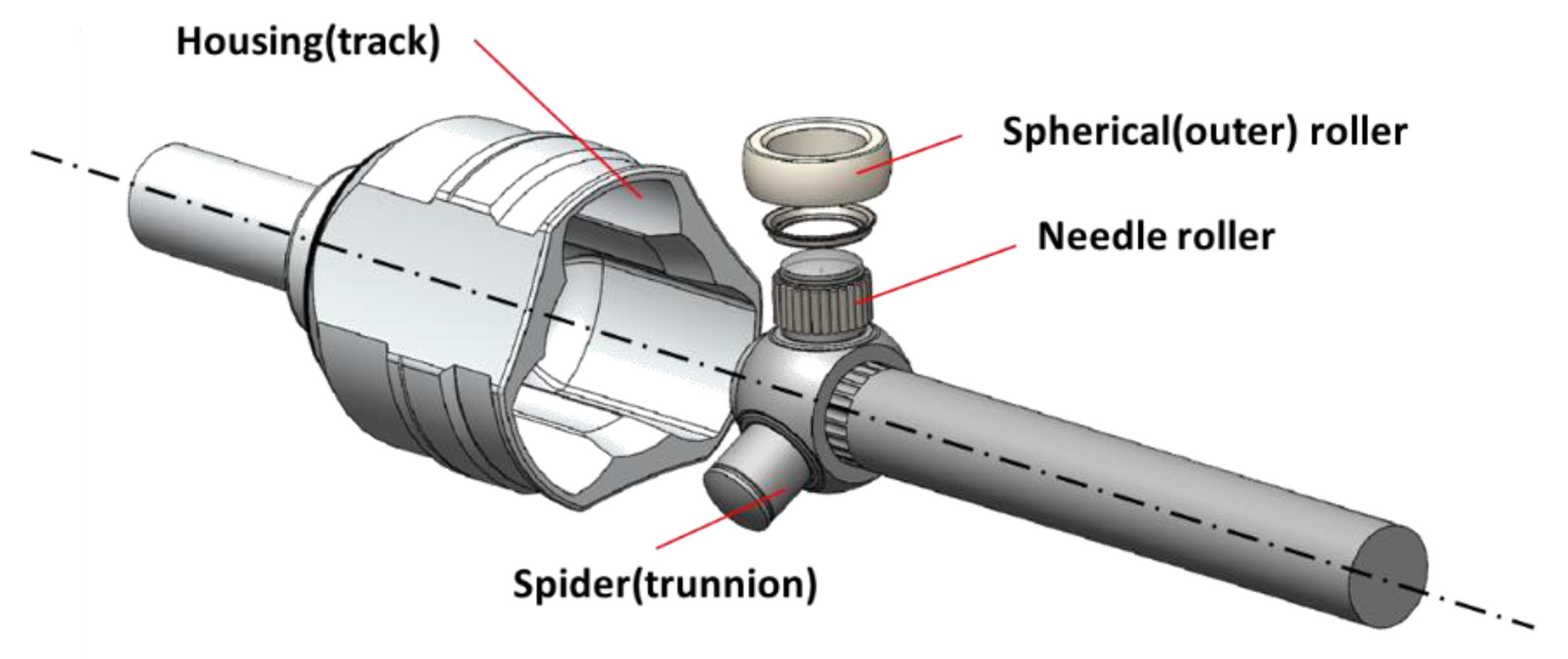
Figure 1 shows a tripod type. It has three spherical rollers—the key feature that distinguishes the tripod from the ball type. Each spherical roller is fixed on the arm of the spider (trunnion) so they maintain a 120° angle difference with each other [3]. In the tripod type, nine contact points occur between the components, and generated axial force (GAF) is induced by the internal friction at the contact points [4]. This causes lateral vibration called ‘shudder effect’ in the vehicle when the vehicle starts to accelerate.

Many studies have been performed to theoretically analyze and reduce the GAF. Watanabe studied kinematics and statics of tripod CVJs [5]. In his study, the closed-loop equations of three spherical rollers, three spider ends and the housing of the CVJ were deduced as spatial mechanism. Serveto proposed analytical and sophisticated GAF models using Adams software [6]. The results were compared with the measurement results. For a further study, Serveto also studied the internal friction of ball CVJs [7]. Lee developed a physics-based phenomenological dynamic friction model of a CVJ [8]. The experimental data and physical parameters were used to develop the model. Mariot developed mechanical models for tripod and ball CVJs [9]. Along with the friction between the rollers and tulip ramps, the friction between the spherical rollers and trunnions was also modeled using viscous and Coulomb friction approaches.

Jo developed a GAF model of a tripod CVJ with theoretical and experimental approaches [10]. The kinematics and friction characteristics were analyzed, and the results were used for the GAF model. In the study, the pure sliding and rolling-sliding friction models were employed to find accurate friction coefficients. Based on the GAF model, the GAF of a CVJ is estimated, and the results are verified by experimental results.

This study proposes a theoretical approach that optimizes design parameters of a CVJ to reduce the GAF. Key design parameters can be found by analyzing the sensitivity of the design parameters on the GAF, and then they are optimized to reduce the GAF. Based on the developed model, the GAF with the optimized parameters is estimated. Then, the estimated results with the optimized parameters are verified by experimental results.

2. GAF Model

2.1. Kinematic Analysis

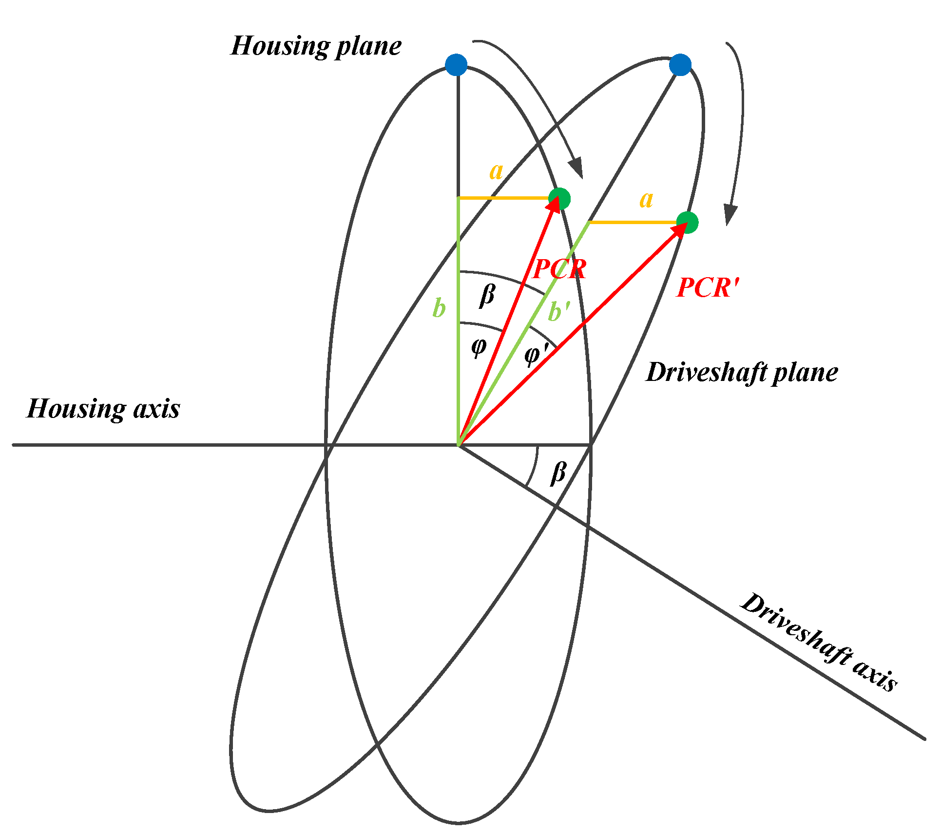
When a tripod CVJ rotates under an articulated condition, the housing axis does not match the driveshaft axis, so they do not rotate with respect to the same axis. To find the contact points between the components, their relative coordinates need to be defined. For these reasons, the kinematics of the CVJ needs to be analysed.

In a tripod CVJ, three spherical rollers have a 120° angle difference. The coordinate system of the housing is transformed to the coordinate system of the spherical roller center by Equation (1).

$${\left(\begin{array}{c}x\\ y\\ z\end{array}\right)}_{Spherical roller}={\left(\begin{array}{ccc}cos\left(-\beta \right)& sin\left(-\beta \right)& 0\\ -sin\left(-\beta \right)& cos\left(-\beta \right)& 0\\ 0& 0& 1\end{array}\right)}^{-1}{\left(\begin{array}{ccc}1& 0& 0\\ 0& cos {\phi }^{\prime }& \sin {\phi }^{\prime }\\ 0& -\sin {\phi }^{\prime }& cos {\phi }^{\prime }\end{array}\right)}^{-1}\left(\begin{array}{c}0\\ PC{R}^{\prime }\\ 0\end{array}\right)$$

(1)

where β = articulation angle, ${\phi }^{\prime }$ = phase angle of driveshaft, $PC{R}^{\prime }$ = pitch circle radius of driveshaft.

As shown in Figure 2, ${\phi }^{\prime }$ is calculated with $a$, $b$ and $b^{\prime }$ by the following equations.

$$a=PCR\sin \phi$$

(2)

$$b=PCR\cos \phi =b^{\prime }\cos \beta$$

(3)

$$tan {\phi }^{\prime }=\frac{a}{b^{\prime }}=\frac{PCR\sin \phi }{\frac{b}{\cos \beta }}=\frac{\sin \phi \cos \beta }{\cos \phi }=\tan \phi \cos \beta$$

(4)

where $\phi$ = phase angle of housing, $PCR$ = pitch circle radius of housing.

As the tripod CVJ rotates, $PC{R}^{\prime }$ creates an elliptical shape with respect to the trunnion axis. $PC{R}^{\prime }$ is calculated by the following equation.

$$PC{R}^{\prime }=\frac{PC{R}^2}{\cos \beta \sqrt{{\left(PCR\cos {\phi }^{\prime }\right)}^2+{\left(\frac{PCR}{\cos \beta }\sin {\phi }^{\prime }\right)}^2}}$$

(5)

Consequently, the coordinate of the spherical roller center is

$${\left(\begin{array}{c}x\\ y\\ z\end{array}\right)}_{Spherical roller}=\left(\begin{array}{c}\frac{PC{R}^2\tan \beta \cos ({\tan }^{-1}(\tan \phi \cos \beta )+\psi )}{\sqrt{{(PCR\cos \left({\tan }^{-1}(\tan \phi \cos \beta )+\psi \right))}^2+{\left(\frac{PCR}{\cos \beta }\sin ({\tan }^{-1}(\tan \phi \cos \beta )+\psi )\right)}^2}}\\ \frac{PC{R}^2\cos ({\tan }^{-1}(\tan \phi \cos \beta )+\psi )}{\sqrt{{\left(PCR\cos ({\tan }^{-1}(\tan \phi \cos \beta )+\psi )\right)}^2+{\left(\frac{PCR}{\cos \beta }\sin \left({\tan }^{-1}(\tan \phi \cos \beta )+\psi \right)\right)}^2}}\\ \frac{PC{R}^2\sin ({\tan }^{?1}(\tan \phi \cos \beta )+\psi )}{\cos \beta \sqrt{{(PCR\cos \left({\tan }^{-1}(\tan \phi \cos \beta )+\psi \right))}^2+{(\frac{PCR}{\cos \beta }\sin ({\tan }^{-1}(\tan \phi \cos \beta )+\psi ))}^2}}\\ \end{array}\right)$$

(6)

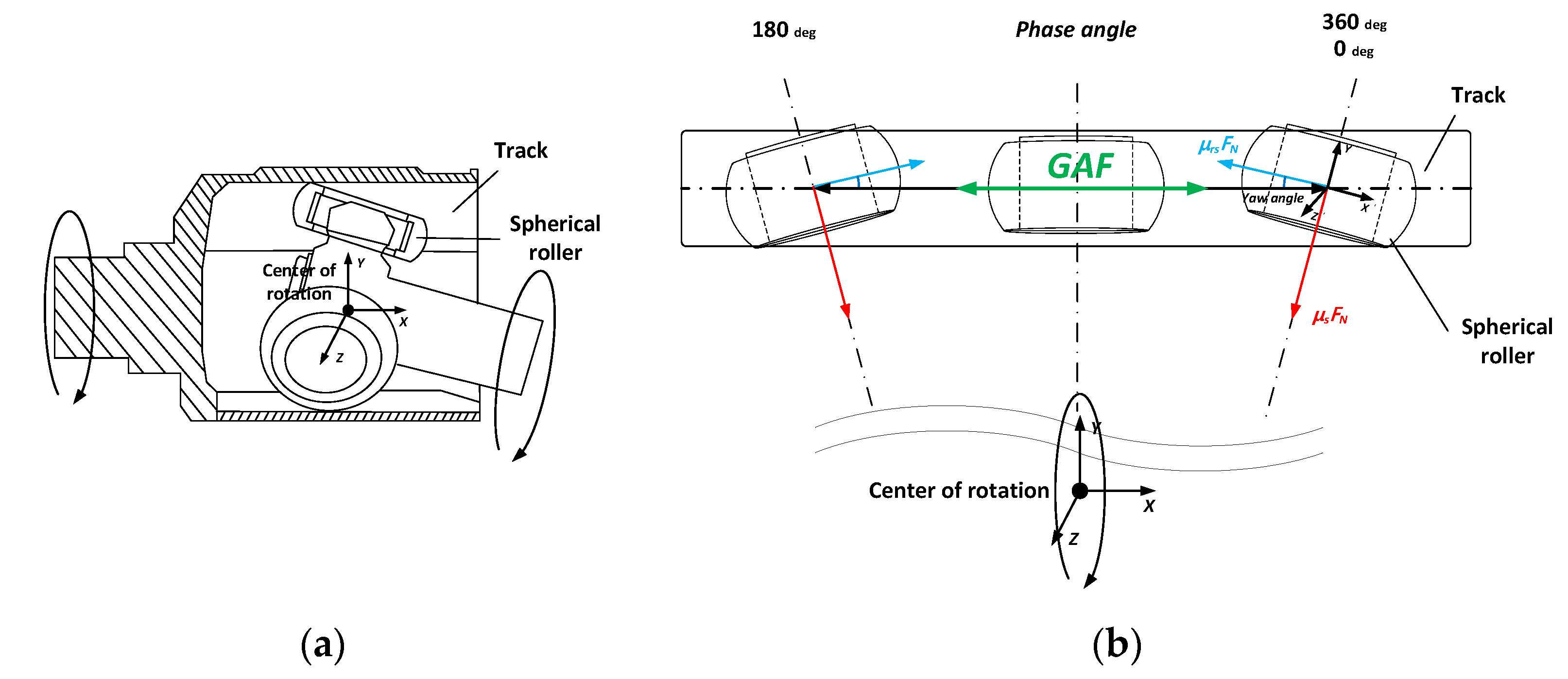
There are two point contacts between the track and the spherical roller. When the CVJ rotates, they make a reciprocating yaw motion on the track, and it creates a yaw angle as shown in Figure 3. The yaw angle is

$$\alpha ={\cos }^{-1}\frac{PCR}{PC{R}^{\prime }}={\cos }^{-1}\left(\cos \beta \sqrt{\begin{array}{c}{\left(\cos \left({\tan }^{-1}\left(\tan \phi \cos \beta \right)+\psi \right)\right)}^2+\\ {\left(\frac{\sin \left({\tan }^{-1}\left(\tan \phi \cos \beta \right)+\psi \right)}{\cos \beta }\right)}^2\end{array}}\right)$$

(7)

where α = yaw angle.

Each spherical roller makes a reciprocating linear motion along the tracks, so one spherical roller has four contact points on the track surface, two on the left side and the other two on the right side. They are calculated by the following equations.

$${\left(\begin{array}{c}x\\ y\\ z\end{array}\right)}_{Spherical-track, left}=\left(\begin{array}{c}\frac{PC{R}^2\tan \beta \cos \left({\tan }^{-1}\left(\tan \phi \cos \beta \right)+\psi \right)}{\sqrt{{\left(PCR\cos \left({\tan }^{-1}\left(\tan \phi \cos \beta \right)+\psi \right)\right)}^2+{\left(\frac{PCR}{\cos \beta }\sin \left({\tan }^{-1}\left(\tan \phi \cos \beta \right)+\psi \right)\right)}^2}}\\ PCR\cos \phi +r_s\cos \mathsf{\delta }\sin \phi +r_s\sin \mathsf{\delta }\cos \phi \\ PCR\sin \phi -r_s\cos \mathsf{\delta }\cos \phi +r_s\sin \mathsf{\delta }\sin \phi \end{array}\right)$$

(8)

$${\left(\begin{array}{c}x\\ y\\ z\end{array}\right)}_{Spherical-track, right}=\left(\begin{array}{c}\frac{PC{R}^2\tan \beta \cos \left({\tan }^{-1}\left(\tan \phi \cos \beta \right)+\psi \right)}{\sqrt{{\left(PCR\cos \left({\tan }^{-1}\left(\tan \phi \cos \beta \right)+\psi \right)\right)}^2+{\left(\frac{PCR}{\cos \beta }\sin \left({\tan }^{-1}\left(\tan \phi \cos \beta \right)+\psi \right)\right)}^2}}\\ PCR\cos \phi +r_s\cos \mathsf{\delta }\sin \phi -r_s\sin \mathsf{\delta }\cos \phi \\ PCR\sin \phi -r_s\cos \mathsf{\delta }\cos \phi -r_s\sin \mathsf{\delta }\sin \phi \end{array}\right)$$

(9)

where $\delta$ = contact angle, $r_{s }$ = radius of spherical roller.

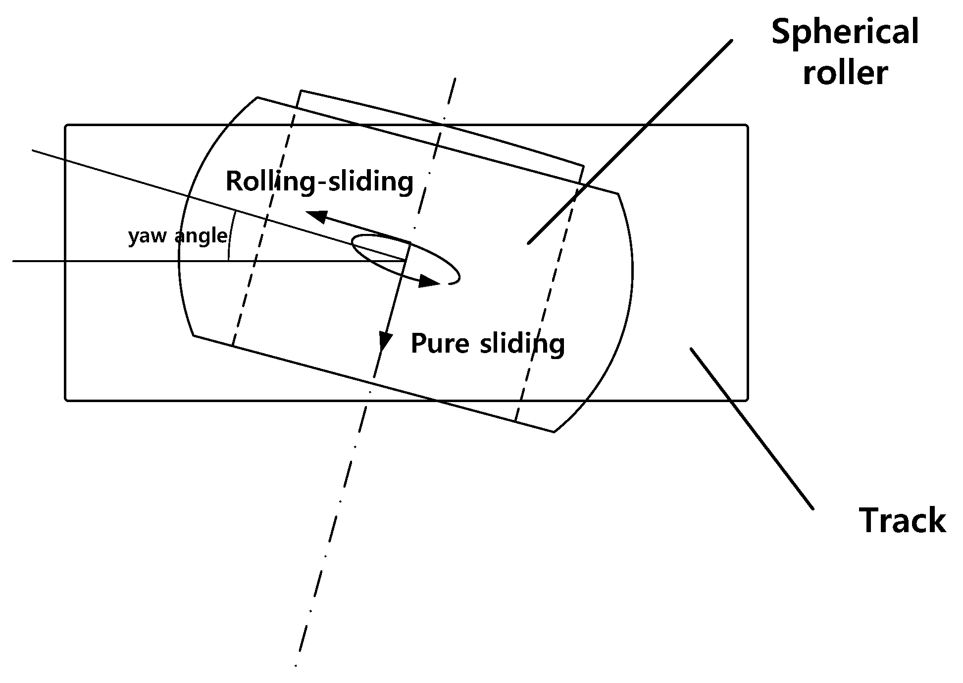
When a tripod CVJ rotates, two types of motions simultaneously occur between the track and the spherical roller—pure sliding and rolling-sliding [11]. Along with the contact points obtained from Equations (8) and (9), the sliding velocity is also required to determine the friction coefficients at the contact points because it is a key factor for the friction characteristics. As well as pure sliding, rolling-sliding simultaneously occur (Figure 4) [11,12,13,14]. The pure sliding motion occurs with respect to the trunnion axis whereas the rolling-sliding motion occurs with respect to the radial direction of the spherical roller. For a spherical roller, its translation velocity is

$$\begin{array}{c}\frac{PC{R}^2\tan \beta \cos ({\tan }^{-1}(\tan {\phi }_{i+1}\cos \beta )+\psi )}{\sqrt{{(PCR\cos \left({\tan }^{-1}(\tan {\phi }_{i+1}\cos \beta )+\psi \right))}^2+{\left(\frac{PCR}{\cos \beta }\sin ({\tan }^{-1}(\tan {\phi }_{i+1}\cos \beta )+\psi )\right)}^2}}-\\ V_t=\frac{\frac{PC{R}^2\tan \beta \cos \left({\tan }^{-1}\left(\tan {\phi }_i\cos \beta \right)+\psi \right)}{\sqrt{{\left(PCR\cos \left({\tan }^{-1}\left(\tan {\phi }_i\cos \beta \right)+\psi \right)\right)}^2+{\left(\frac{PCR}{\cos \beta }\sin \left({\tan }^{-1}\left({\phi }_i\cos \beta \right)+\psi \right)\right)}^2}}}{t}\end{array}$$

(10)

where $V_t$ is translation velocity.

Actual sliding velocity is the product of translation velocity and rolling—sliding ratio, so it is calculated by the following equation.

$$V_s=\gamma V_t$$

(11)

where $V_s$ is actual sliding velocity.

2.2. Contact Points

Each spherical roller is in contact with the tracks. As a result, normal load occurs at the contact points. To calculate the normal load, the applied torque to the driving shaft and the coordinates of the contact points are required. It is calculated by the following equations.

$$N_1{r}_1+N_2{r}_2+N_3{r}_3=T$$

(12)

$$\overrightarrow{N_1}+\overrightarrow{N_2}+\overrightarrow{N_3}=0$$

(13)

$$r_t=\sqrt{\begin{array}{c}{\left(\frac{PC{R}^2\cos ({\tan }^{-1}(\tan \phi \cos \beta )+\psi )}{\sqrt{{\left(PCR\cos ({\tan }^{-1}(\tan \phi \cos \beta )+\psi )\right)}^2+{\left(\frac{PCR}{\cos \beta }\sin \left({\tan }^{-1}(\tan \phi \cos \beta )+\psi \right)\right)}^2}}\right)}^2\\ +{\left(\frac{PC{R}^2\sin ({\tan }^{?1}(\tan \phi \cos \beta )+\psi )}{\cos \beta \sqrt{{(PCR\cos \left({\tan }^{-1}(\tan \phi \cos \beta )+\psi \right))}^2+{(\frac{PCR}{\cos \beta }\sin ({\tan }^{-1}(\tan \phi \cos \beta )+\psi ))}^2}}\right)}^2\end{array}}$$

(14)

where $r_1$,$r_2$,$r_3$ = moment arms from CVJ center to spherical roller center, $N_1$,$N_2$,$N_3$ = normal loads at contact points.

In order to calculate the contact areas from the normal load and curvature, Hertz’s theory is introduced [15,16]. A point contact between the track and the spherical roller occurs and its contact area is assumed to be an ellipse shape [11,15]. Accordingly, the equivalent radius is calculated by the following equation.

$$R_{eq1}={\left(\frac{1}{R_1}+\frac{1}{R_3}\right)}^{-1}=\frac{R_1{R}_3}{R_1+R_3}$$

(15)

$$R_{eq2}={\left(\frac{1}{R_2}+\frac{1}{R_4}\right)}^{-1}=\frac{R_2{R}_4}{R_2+R_4}$$

(16)

where $R_{eq1},R_{eq2}$ = equivalent radius,$R_1,R_3$ = radius of curvature1, $R_2,R_4$ = radius of curvature2.

The contact area is

$$A=\pi ab=\pi \sqrt[3]{{\left(\frac{3N}{4E_{eq}}\right)}^2{R}_{eq1}{R}_{eq2}}$$

(17)

where $A$ = contact area, $a, b$ = semi minor and major axes of contact area.

In Equation (17), the equivalent Young’s modulus is

$$E_{eq}={\left(\frac{1-{\nu }_1{}^2}{E_1}+\frac{1-{\nu }_2{}^2}{E_2}\right)}^{-1}$$

(18)

where $v_1$ = Poisson’s ratio1, $E_1$ = Young’s modulus1, $v_2$ = Poisson’s ratio2, $E_2$ = Young’s modulus2, $E_{eq}$ = equivalent Young’s modulus.

Consequently, the mean contact pressure at the contact point is

$$P=\pi \sqrt[3]{{\left(\frac{4E_{eq}}{3}\right)}^2\frac{N}{R_{eq1}{R}_{eq2}}}$$

(19)

2.3. Friction Coefficients

As mentioned in Section 2.1, the GAF is produced by pure sliding and rolling-sliding between the track and the spherical roller. Hence, both motions should be considered to establish an accurate GAF model. Especially for the rolling-sliding motion, rolling-sliding ratio is required along with friction coefficient whereas only friction coefficient is required for the pure sliding.

The pure sliding occurs with respect to the trunnion axis whereas the rolling-sliding occurs with respect to the radial direction of the spherical roller. Equations (20)–(22) represents the friction forces due to the friction coefficients of pure sliding and rolling-sliding.

$$F_s={\mu }_s{N}_{st}$$

(20)

$$F_{rs}={\mu }_{rs}{N}_{st}$$

(21)

$${\mu }_{rs}=\frac{l_s}{l_t}{\mu }_s$$

(22)

where $F_s$ = friction force of pure sliding, ${\mu }_s$ = friction coefficient of sliding, $N_{st}$ = normal force between track and spherical roller, $F_{rs}$ = friction force of rolling-sliding, ${\mu }_{rs}$ = friction coefficient of rolling-sliding, $\gamma$ = rolling-sliding ratio, $l_t$ = total travelling distance of spherical roller, $l_s$ = sliding distance of spherical roller.

As in Equation (22), the friction coefficient of rolling-sliding is the product of sliding friction coefficient and rolling-sliding ratio [13,17]. From a theoretical point of view, the rolling-sliding ratio is very difficult to estimate because it varies with the driving conditions. Accordingly, in the previous study, it was measured by a measurement system [10]. In addition, the friction coefficients between the track and the spherical roller were also measured using a tribometer as they are determined by sliding velocity, contact pressure and lubricant [18,19].

2.4. Generated Axial Force Model

From the theoretical and experimental approaches previously described, all information that is required to build a complete GAF model can be obtained. As a spherical roller moves on the track, an axial force is produced, and it varies with the spherical roller’s phase angle. As a result, the GAF can be modeled by Equation (23).

$$GAF={\displaystyle \sum }_{i=1}^3{\mu }_s{N}_{st}sin\left({\alpha }_i\right)sign\left|V_{t\_z}\right|+{\mu }_{rs}{N}_{st}cos\left({\alpha }_i\right)sign\left|V_{t\_x}\right|$$

(23)

The first term represents the sliding friction force produced along the trunnion axis and the second term represents the rolling-sliding friction force produced along the radial direction of the spherical roller. These forces change directions as the spherical roller makes reciprocal motions on the track, so the equation has two sign terms whose values are determined by the direction. When the spherical roller moves in the positive Z-direction, the sign of the first term is positive. In the same manner, when moving in the positive X-direction, the sign of the second term is positive. In the second term, ${\mu }_{rs}$ is the product of the rolling-sliding ratio and the friction coefficient of pure sliding. The rolling-sliding ratio is between 0 and 1, so ${\mu }_{rs}$ is always smaller than ${\mu }_s$.

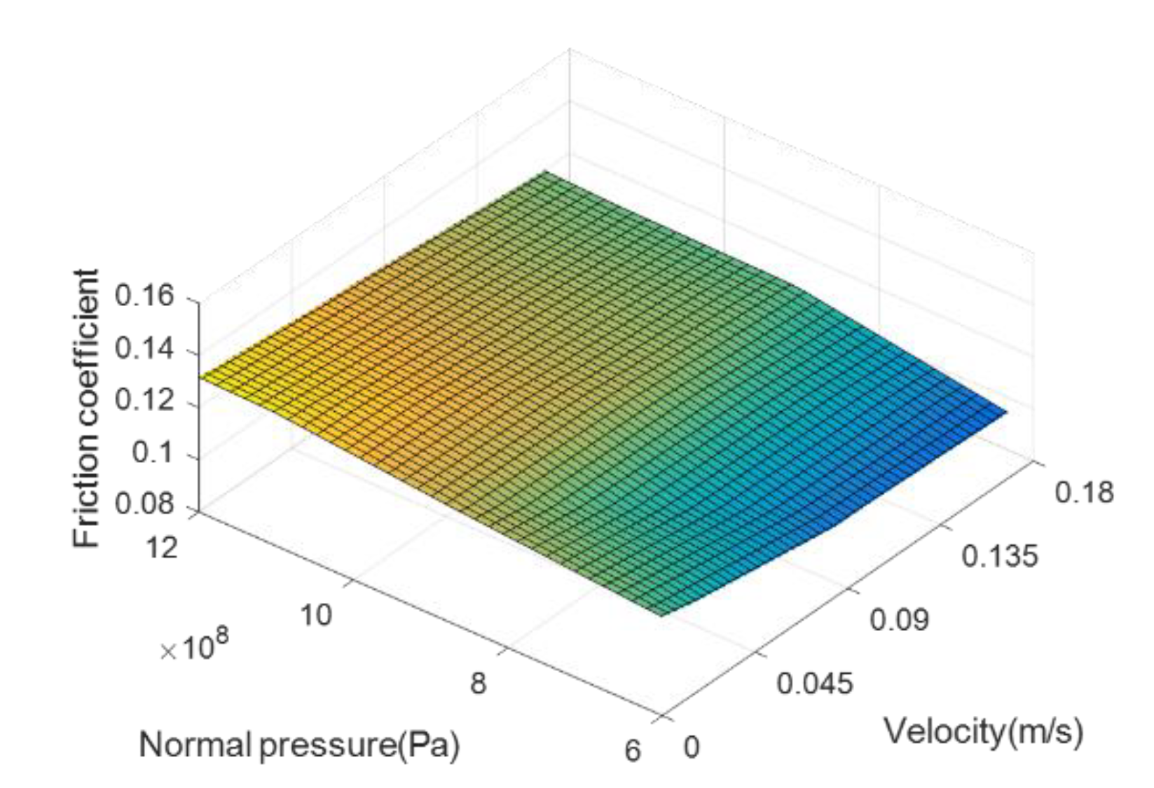
From Equation (23), it is known that the main parameters of GAF are normal force and friction coefficient. Among these parameters, friction coefficient is the only parameter that can be managed by design modification since normal force is determined by driving conditions. GAF comprises of the rolling-sliding and pure sliding terms, and the rolling-sliding term comprises of the friction coefficients of pure sliding and the rolling-sliding ratio. Accordingly, the main parameters that determine GAF are these friction coefficients.

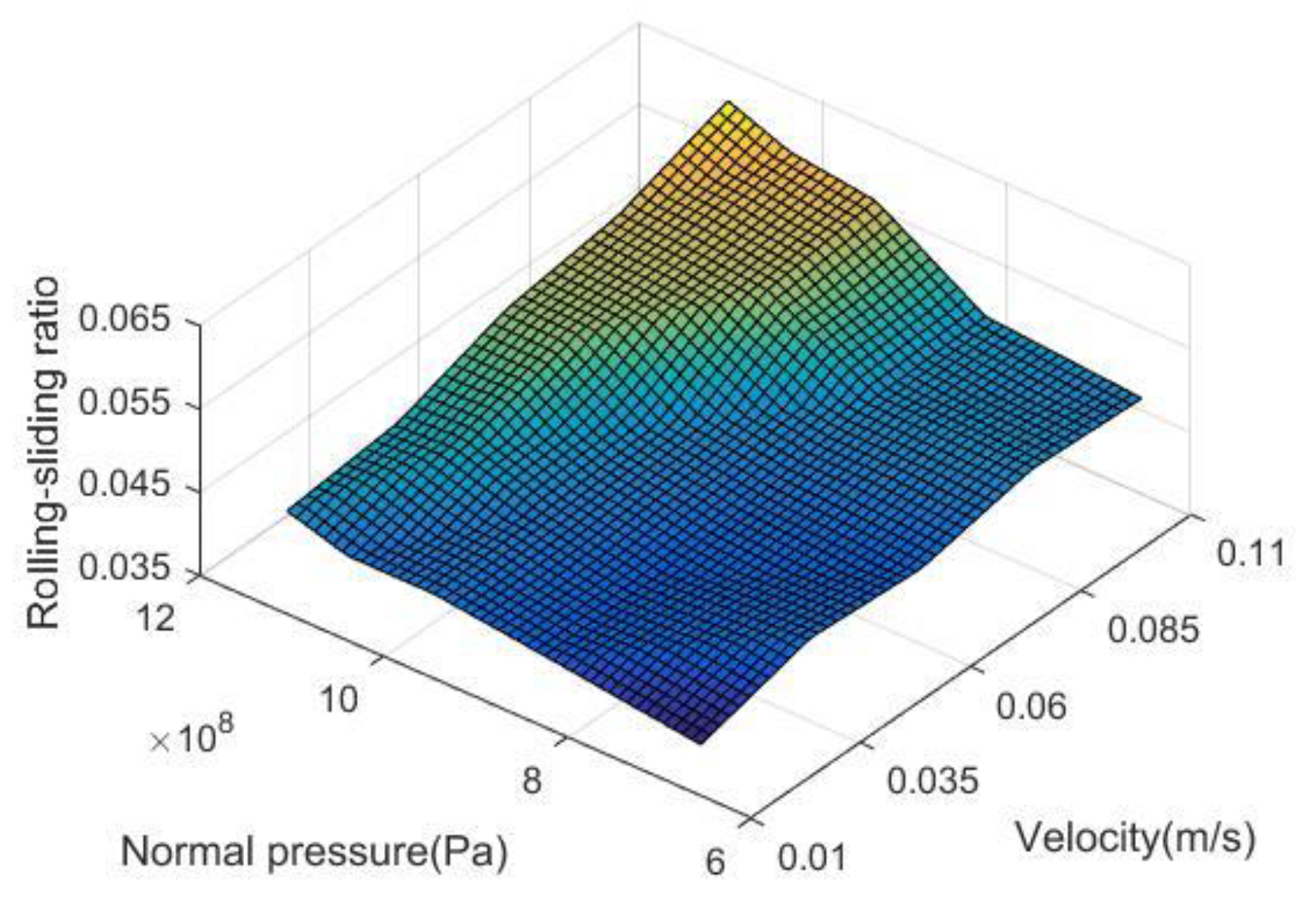
From the previous study, the friction coefficient of pure sliding and the rolling-sliding ratio are mainly determined by sliding velocity and normal pressure [10]. Figure 5 and Figure 6 show the friction coefficient of pure sliding and the rolling-sliding ratio between the track and the spherical roller, respectively. As shown, both rolling sliding ratio and friction coefficient are proportional to normal pressure. On the other hand, friction coefficient is inversely proportional to sliding velocity whereas rolling sliding ratio is proportional.

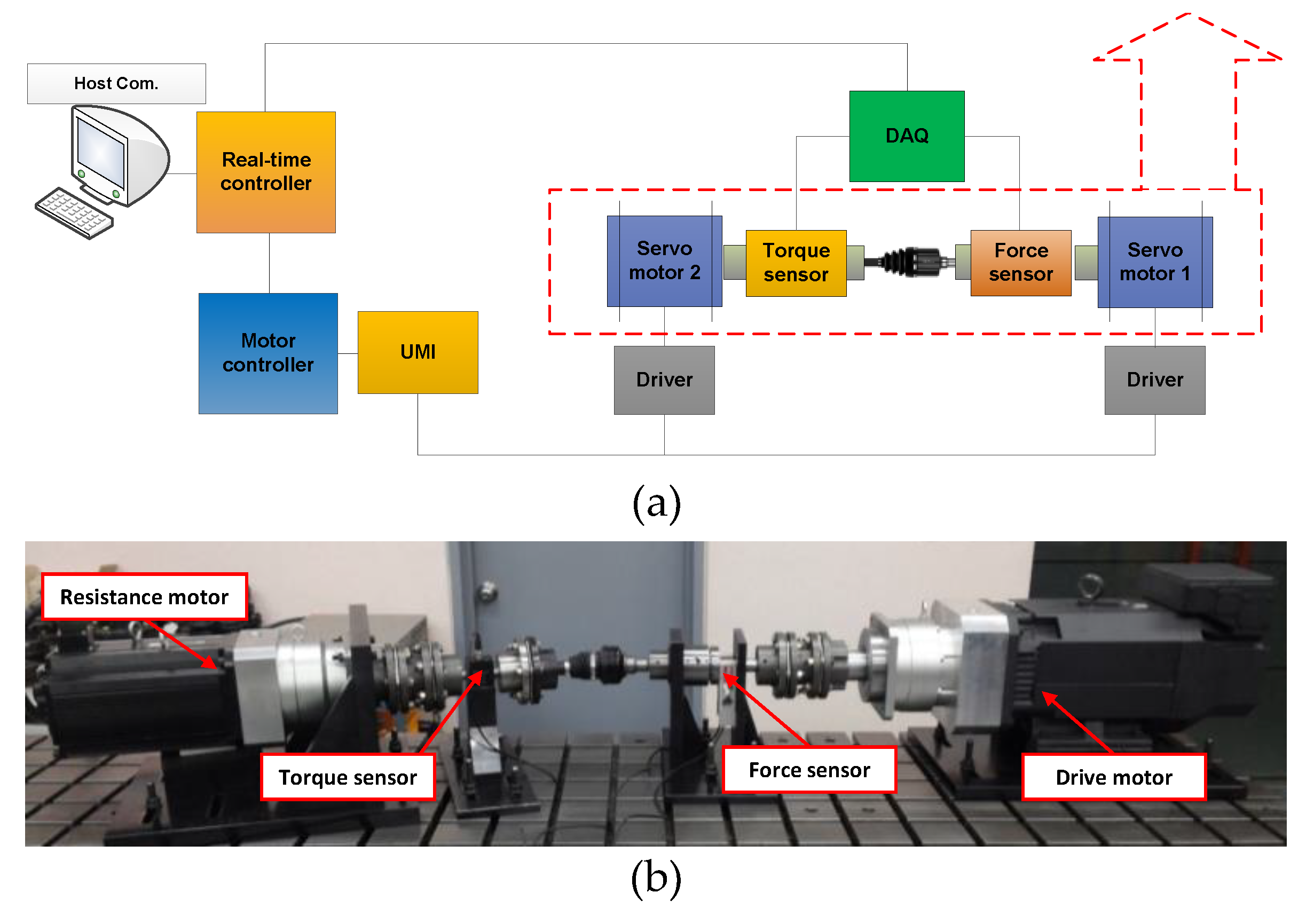
3. Measurement System

For verification, a system is set up to measure the GAF. This system measures the GAF of a CVJ with various design parameters and the results are compared with the estimation results by the model. As shown in Figure 7, two servo motors—driving and resistant motors—are located at both ends of the system. The driving motor applies driving torque and the resistant motor applies resistant torque to the CVJ. There is a torque sensor between the resistant motor and the CVJ to measure the applied torque. Correspondingly, there is a force sensor between the driving motor and the CVJ to measure the generated GAF. Measured torque by the torque sensor is converted to normal pressure at the contact points so the experiment conditions are controlled according to the driving conditions. Labview and MATLAB are utilized to program the system.

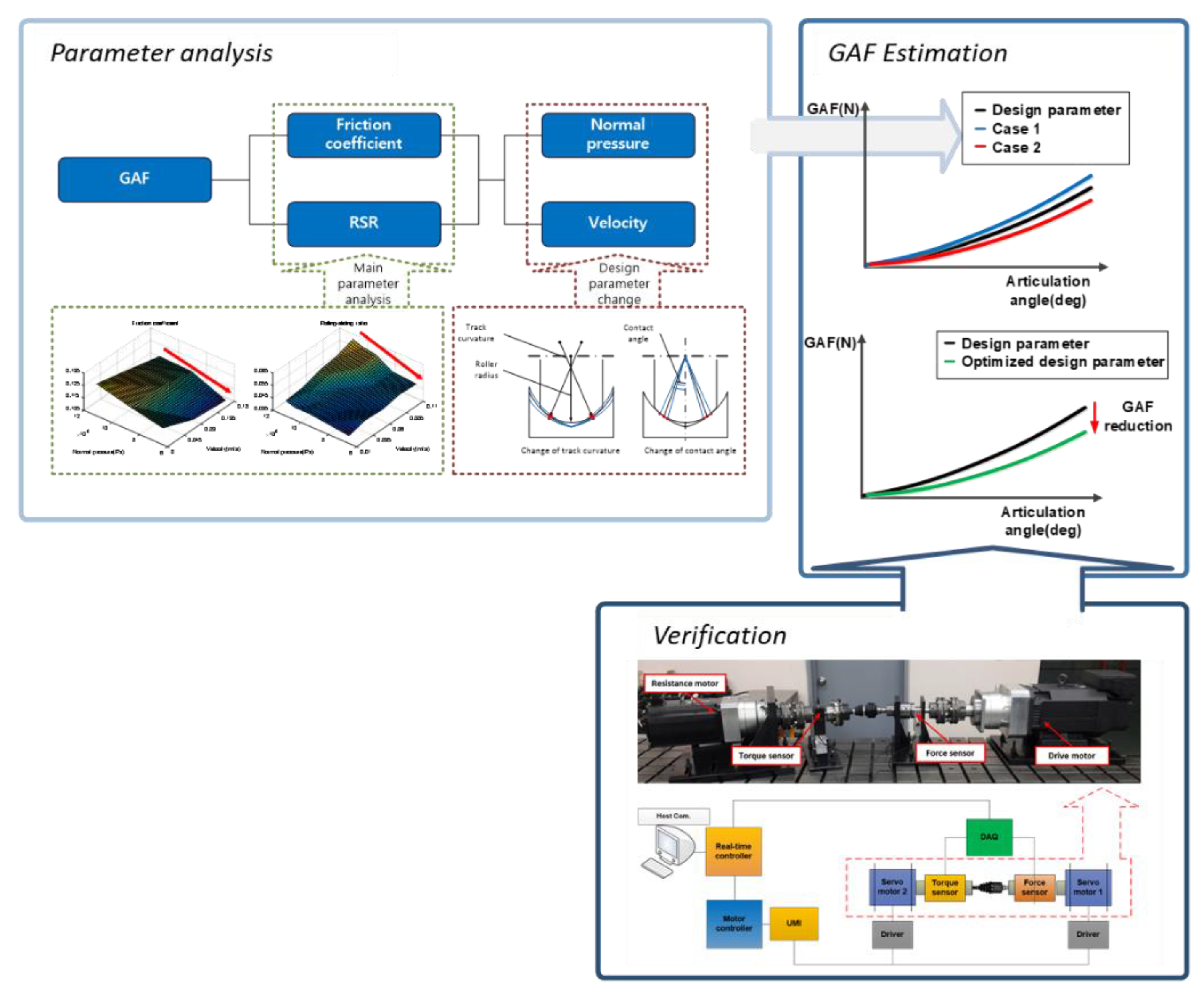
4. Methodology

Figure 8 shows the methodology for GAF reduction. First, a CVJ is designated and its parameter analysis on the GAF is performed based on the developed model. When a CVJ rotates under a driving condition, sliding velocity can be controlled only by modifying the entire size of the CVJ. Because sliding velocity varies with the pitch circle radius which affects the joint size. Accordingly, the effect of sliding velocity is not considered in this study. Normal pressure at the contact points, on the other hand, is determined by the joint design parameters and the driving conditions. Although the driving conditions cannot be controlled, design parameters such as track curvature and contact angle can be controlled within a certain range without changing the joint size. Considering the design constraints of the CVJ and the manufacturing difficulties, the design parameters are changed within limited ranges as shown in

Table 1. Design parameter variation.

Design Parameter	Existing Value	Changed Value
Contact angle (deg)	10	8 (−20%), 12 (+20%)
Track curvature (mm)	44.2	35.36 (−20%), 39.78 (−10%), 48.62 (+10%), 53.04 (+20%)

.

Based on the parameter analysis results, the GAF with various design parameters is estimated by the developed model, and then the results are verified by comparing them with the measurement results.

5. Results and Discussion

5.1. Parameter Analysis by the Model

5.1.1. Contact Angle

Figure 9a shows the normal pressure change with respect to contact angle and driving torque. As expected, normal pressure increases as driving torque increases. However, the contact angle does not have a large influence on normal pressure. Figure 9b shows the normal pressure change with respect to contact angle at 400 Nm and 200 rpm condition.

5.1.2. Track Curvature

Figure 10a shows the normal pressure change with respect to track curvature and driving torque. As shown, normal pressure rapidly increases with the increase of track curvature. +20% of track curvature has the largest normal pressure at all driving torque whereas −20% has the smallest normal pressure. Throughout the entire driving torque, the decrement of normal pressure is larger than its increment with the change of track curvature as shown in Figure 10b. Figure 10b shows the normal pressure variation with respect to the track curvature at 400 Nm and 200 rpm condition. +10% of track curvature shows a normal pressure increase by 0.98 while −10% shows a decrease by 1.28. +20% shows a normal pressure increase by 1.52 while −20% shows a decrease by 3.68.

As known from the results, a CVJ with +20% contact angle and −20% track curvature has the lowest normal pressure at all driving conditions. Furthermore, it can be expected that the CVJ will also have the lowest GAF at all driving conditions, compared to the CVJs with the other design parameters.

5.2. GAF Reduction

In the previous section, parameter analysis on the GAF was carried out based on the developed model. The GAF with different design parameters can be also estimated by the GAF model to find the amount of GAF reduction by the design parameter changes.

5.2.1. GAF Reduction by the Model

GAF estimation with the various design parameters is carried out using the model. Figure 11 shows the GAF at 200 rpm with respect to driving torque. Regardless of the design parameter changes, GAF is proportional to driving torque. As expected from the normal pressure change results, the contact angle and track curvature also affect the GAF. As the normal pressure change results, GAF is proportional to track curvature and inversely proportional to contact angle. Furthermore, GAF is more affected by track curvature than contact angle like normal pressure. With the change of track curvature, GAF at 100 Nm changes from 7.99 to 8.59 N whereas it changes from 8.34 to 8.42 with the contact angle. This GAF change increases as driving torque increases, and eventually it is the most noticeable at 400 Nm. With the change of track curvature, GAF changes from 33.96 to 37.63 N whereas it changes from 37.13 to 37.49 N with the contact angle. At all driving torque, the GAF differences with the track curvature are much larger than the GAF differences with the contact angle.

From the estimation results, the optimized design parameter is +20% contact angle and −20% track curvature where the CVJ has the lowest GAF as shown in Figure 11. Figure 12 shows the GAF variation at 400 Nm with respect to contact angle and track curvature. As in Figure 12a, GAF noticeably drops with the decrease of track curvature whereas it slightly rises with the increase of track curvature. On the other hand, contact angle hardly affects GAF as shown in Figure 12b.

5.2.2. GAF Measurement and Comparison

Table 2. GAF verification conditions.

Torque (Nm)	400
Rotational speed (rpm)	200
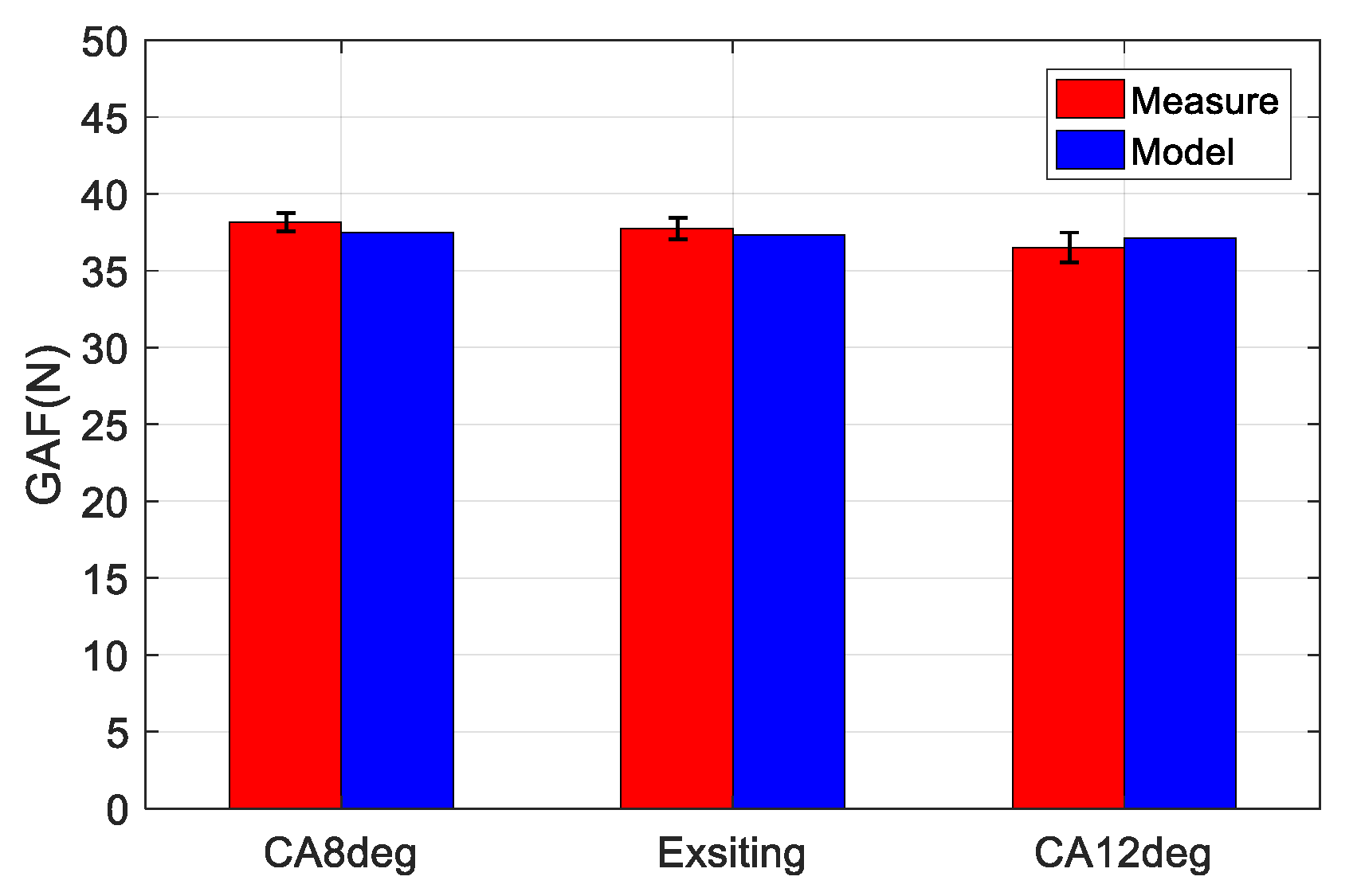
Articulation angle (deg)	12

shows the experimental conditions for the GAF measurement and Figure 13 shows the estimation and measurement results according to the contact angle. As seen from the estimation results in Figure 12a, contact angle variation does not make noticeable changes to GAF. The measurement and the estimation have the same trend with the change of contact angle in that GAF slightly decreases as contact angle increases. The measured GAF change is from 36.52 to 38.16 N whereas the estimated GAF change is from 37.13 to 37.50 N. The minimum and maximum differences between the measurement and the estimation (measurement-estimation) are −0.62 and 0.67 N, respectively. From the verification results with respect to contact angle, it is obvious that contact angle does not have a large influence on GAF.

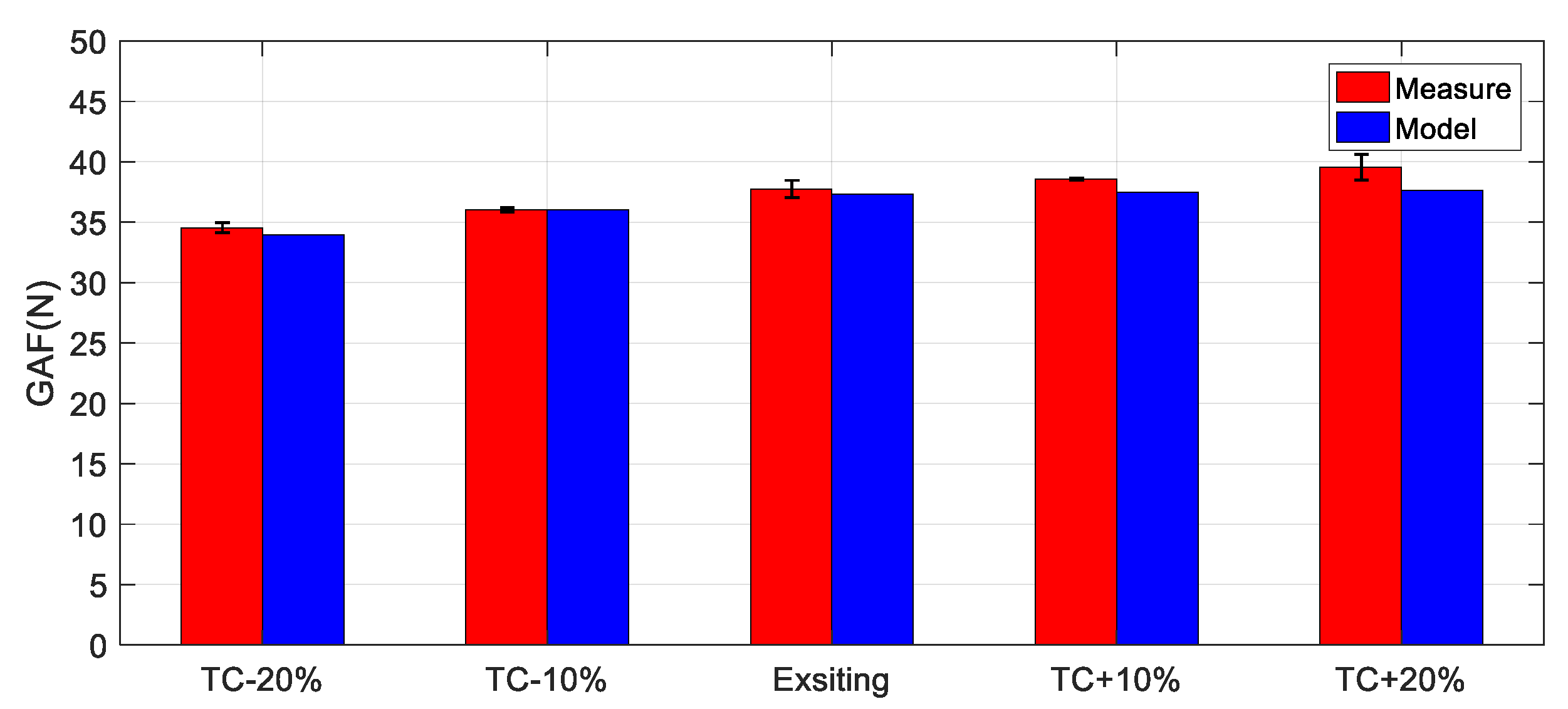
Figure 14 shows the estimation and measurement results according to track curvature. Like the estimation, track curvature is controlled from −20 to 20% with 10% increments because track curvature has a large influence on normal pressure. As shown in Figure 14, the measurement and the estimation show the same trend with the change of track curvature in that both results increase with the track curvature. The measured GAF change is from 34.56 to 39.56 N whereas the estimated GAF change is from 33.97 to 37.62 N. The minimum and maximum differences between the measurement and the estimation (measurement-estimation) are 0 and 1.94 N, respectively. The verification results show that track curvature is a key factor for the GAF.

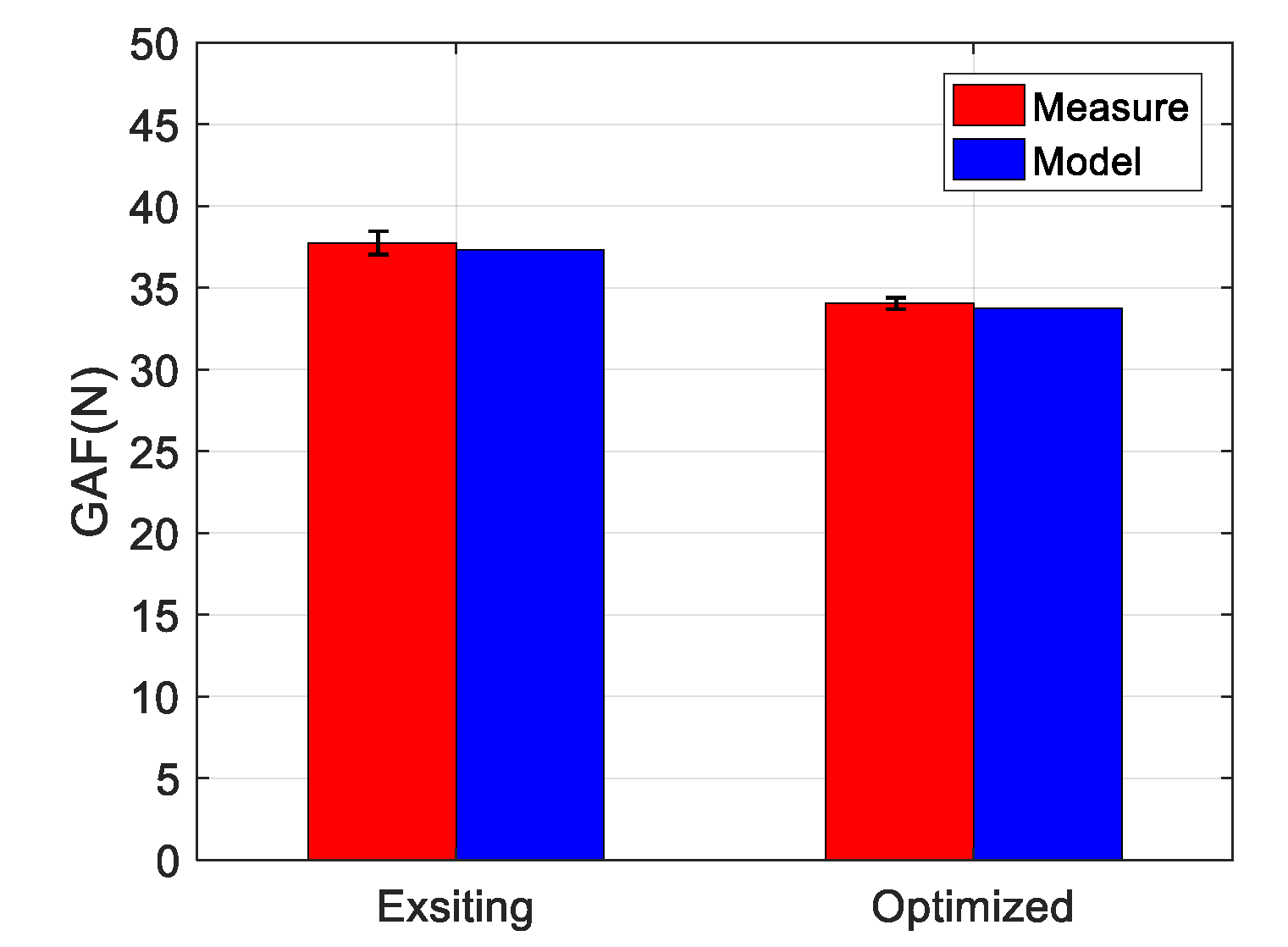
Based on the results, the optimized design parameter that causes the maximum GAF reduction is +20% contact angle and −20% track curvature. Figure 15 shows the GAF comparison results between the existing and optimized design parameters. According to the measurement results, the GAF with the optimized design parameter is 34.05 N whereas it is 37.77 N with the existing parameter. The GAF reduction is 3.72 N, which is −9.85%.

6. Conclusions

An experimental and numerical study to reduce GAF of a tripod CVJ is presented in this study. Based on the complete GAF model, which has been developed from the kinematic and friction coefficient analysis on the tripod CVJ, the parameter analysis is carried out to find the key parameters of the GAF. Then, design optimization analysis is performed to reduce the GAF.

From the GAF model, it can be known that the rolling-sliding ratio and friction coefficient between the track and the spherical roller are the key parameters, and this fact also suggests that GAF can be reduced by decreasing them. These two parameters are related to normal pressure and sliding velocity which are also highly related to design parameters such as track curvature and contact angle. In this study, the track curvature and contact angle of a CVJ were modified and their impact on the GAF is estimated. As track curvature changes from −20 to 20%, GAF increases with the increase of track curvature. On the other hand, GAF does not show significant changes with the change of contact angle.

In this study, the estimation results are compared with the experiment results to verify the estimated GAF reduction. Several tripod CVJs with different design parameters were manufactured, and their GAF was measured. A system was built to measure GAF. The measurement system has force sensors between the CVJ and the servo motors so that they can measure its GAF. From the verification results, the measurement results nearly showed the same results as the estimation, and throughout the entire driving torque range, the GAF has its lowest value at +20% contact angle and −20% track curvature. Finally, the GAF with the optimized design parameters was compared with the GAF with the existing design parameters, which shows 9.85% reduction.

References

- Hillier, V.A.W.; Coombes, P. Fundamentals of Motor Vehicle Technology, 4th ed.; Nelson Thornes: Cheltenham, UK, 1991. [Google Scholar]
- Wagner, E.; Cooney, C. Universal Joint and Driveshaft Design Manual; Society of Automotive Engineers: Warrendale, PA, USA, 1979; pp. 127–129. [Google Scholar]
- Mondragon-Parra, R.E. Life Model for Rolling Contact, Applied to the Optimization of a Tripode Constant Velocity Joint. Ph. D. Thesis, Michigan State University, East Lansing, MI, USA, 2010. [Google Scholar]
- Seherr-Thoss, H.-C.; Schmelz, F.; Aucktor, E. Universal Joints and Driveshafts: Analysis, Design, Applications; Springer: Berlin, Germany, 2006. [Google Scholar]
- Watanabe, K.; Kawakatsu, T.; Nakao, S. Kinematic and static analyses of tripod constant velocity joints of the spherical end spider type. J. Mech. Des. 2005, 127, 1137–1144. [Google Scholar] [CrossRef]
- Serveto, S.; Mariot, J.P.; Diaby, M. Modelling and measuring the axial force generated by tripod joint of automotive drive-shaft. Multibody Syst. Dyn. 2007, 19, 209–226. [Google Scholar] [CrossRef]
- Serveto, S.; Mariot, J.P.; Diaby, M. Secondary torque in automotive drive shaft ball joints: Influence of geometry and friction. Proc. Inst. Mech. Eng. Part K-J. Multi-Body Dyn. 2008, 222, 215–227. [Google Scholar] [CrossRef]
- Lee, C.H.; Polycarpou, A.A. A phenomenological friction model of tripod constant velocity (CV) joints. Tribol. Int. 2010, 43, 844–858. [Google Scholar] [CrossRef]
- Mariot, J.P.; K'Nevez, J.Y.; Barbedette, B. Tripod and ball joint automotive transmission kinetostatic model including friction. Multibody Syst. Dyn. 2004, 11, 127–145. [Google Scholar] [CrossRef]
- Jo, G.H.; Kim, S.H.; Kim, D.W.; Chu, C.N. Estimation of generated axial force considering rolling-sliding friction in tripod-type constant velocity joint. Tribol. Trans. 2018, 61, 889–900. [Google Scholar] [CrossRef]
- Popov, V.L. Contact Mechanics and Friction; Springer: Dordrecht, The Netherlands, 2010. [Google Scholar]
- Hamrock, B.J.; Dowson, D. Ball Bearing Lubrication: The Elastohydrodynamics of Elliptical Contacts; Wiley: New York, NY, USA, 1981. [Google Scholar]
- Bhushan, B. Introduction to Tribology; Wiley: Hoboken, NJ, USA, 2013. [Google Scholar]
- Kalker, J.J. Three-Dimensional Elastic Bodies in Rolling Contact; Springer Science & Business Media: Berlin, Germany, 1990. [Google Scholar]
- Johnson, K.L. Contact Mechanics; Cambridge University Press: Cambridge, UK, 1985. [Google Scholar]
- Johnson, K.; Greenwood, J.; Poon, S. A simple theory of asperity contact in elastohydro-dynamic lubrication. Wear 1972, 19, 91–108. [Google Scholar] [CrossRef]
- Bhushan, B. Principles and Applications to Tribology, 2nd ed.; Wiley: Hoboken, NJ, USA, 2013. [Google Scholar]
- Yamaguchi, Y. Tribology of Plastic Materials: Their Characteristics and Applications to Sliding Components; Elsevier: New York, NY, USA, 1991. [Google Scholar]
- Mizuno, T.; Okamoto, M. Effects of Lubricant Viscosity at Pressure and Sliding Velocity on Lubricating Conditions in the Compression-Friction Test on Sheet Metals. J. Lubr. Technol. -Trans. Am. Socity Mech. Eng. 1982, 104, 53–59. [Google Scholar] [CrossRef]