Article

Analysis of Tidal Accelerations in the Solar System and in Extrasolar Planetary Systems

Department of Physics and Astronomy, Kirchhoff-Institute for Physics, Heidelberg University, Im Neuenheimer Feld 227, 69120 Heidelberg, Germany
*
Authors to whom correspondence should be addressed.
Max Planck Institute for Astronomy, Department Planet and Star Formation (PSF), Königstuhl 17, 69117 Heidelberg, Germany.
Appl. Sci. 2021, 11(18), 8624; https://doi.org/10.3390/app11188624
Submission received: 18 July 2021 / Revised: 13 September 2021 / Accepted: 14 September 2021 / Published: 16 September 2021
(This article belongs to the Topic Dynamical Systems: Theory and Applications)

Abstract

:

Featured Application

The article is presenting simulations for tidal accelerations in multi-body planetary systems under the precondition of having only few physical and orbital parameters experimentally available. Tidal acceleration vectors were calculated under missing most orbital parameters for the solar system as calibration standard and the TRAPPIST-1 system as an extrasolar example.

Abstract

Volcanism powered by tidal forces inside celestial bodies can provide enough energy to keep important solvents for living systems in the liquid phase. A prerequisite to calculate such tidal interactions and consequences is depending on simulations for tidal accelerations in a multi-body system. Unfortunately, from measurements in many extrasolar planetary systems, only few physical and orbital parameters are well-known enough for investigated celestial bodies. For calculating tidal acceleration vectors under missing most orbital parameter exactly, a simulation method is developed that is only based on a few basic parameters, easily measurable even in extrasolar planetary systems. Such a method as the one presented here allows finding a relation between the tidal acceleration vectors and potential heating inside celestial objects. Using the values and results of our model approach to our solar system as a “gold standard” for feasibility allowed us to classify this heating in relation to different forms of volcanism. This “gold standard” approach gave us a classification measure for the relevance of tidal heating in other extrasolar systems with a reduced availability of exact physical parameters. We help to estimate conditions for the identification of potential candidates for further sophisticated investigations by more complex established methods such as viscoelastic multi-body theories. As a first example, we applied the procedures developed here to the extrasolar planetary system TRAPPIST-1 as an example to check our working hypothesis.

1. Introduction

Over the last decades, many objects in the solar system have been identified with liquid oceans powered by tidal heating. Well-known examples are (J1) Io (designation (J1) given in this paper for distinction from asteroid (85) Io), Europa, Enceladus, and Ganymede, among many more. Numerous models have been evolved for description and further analysis, containing various predictions for the interior structure of the examined celestial objects. Most of these models are based on vast and extensive theories of viscoelasticity considering different analytical and numerical models for different oscillation modes and layers forming the inner structure of the celestial body, see, e.g., [1,2]. For more complex models distinguishing oscillation modes and causes for the tidal heat dissipation such as eccentricity, obliquity, and asynchronous spin to orbit rates, see, e.g., [3]. These studies, among many others, provide a very precise determination of custom-fit models for each celestial object, achieving a detailed and deep understanding of the tidal heating processes involved.
In principle, tidal heating or, in more general considerations, tidal interactions happen in all planetary systems known in the universe. An additional specialty in many extrasolar planetary systems, especially in those of the numerous M and K stars, is the very great proximity of planetary objects to each other [4,5,6]. This might already result in an influence the planetary objects have on each other. These additional effects based on multi-body contributions to tidal interactions were so far only rarely considered, especially since all relevant physical parameters required for complex modeling were not available for many extrasolar systems.
Without denying the need for deep and detailed analyses based on complex theoretical approaches as, for instance, the successful viscoelastic multi-body theories mentioned above, it may be of advantage to have a rough calculation procedure whenever the measured data availability does not sufficiently satisfy the theories’ requirements. This may offer a glimpse of potential systems of interest in advance by using a model in which mainly distances between the objects, their radii R, the eccentricities of their orbits e, masses, and other orbital elements are used.
Here, we present a newly developed approach for the simulation of tidal accelerations in systems of celestial objects under multi body conditions, requiring a minimalistic set of experimental physical parameters. The model was first applied to our solar system as a “gold standard” to determine whether this is sufficient to identify candidates for tidal interactions. Our solar system is the best test candidate, because a comparison to precise measurements and models developed for the many objects in the solar system can be made. Often space probes have visited these objects, and accurate investigations have been performed so that the results can be used in some way as a standard to classify other systems so far not investigated in such great details. This may even allow an assessment of whether a certain value found in the model may favor liquid solvents or cryo- or even siliceous volcanism inside the object.
In addition, some aspects of the evolution of the eccentricity e over time have been investigated in this approach. In a final step, this approach has been applied to an extrasolar planetary system, namely TRAPPIST-1 [5,6]. All planets known for this system are included. We further present our results for a simplified version of our simulation, using a smaller set of orbital elements. We compare this simplified version to the original one and outline how this simplified version could be applicable to other extrasolar planetary systems for which usually only a smaller set of orbital elements is known with acceptable accuracy. This could give a first estimate of the potential significance of tidal influences in other less well-known extrasolar systems.
Finally, we discuss this new developed pre-screening method for extrasolar systems, as well as further findings and implications for objects in our solar system.

2. Materials and Methods

To include the possible mutual multi-planetary influences, the forces of all objects on each other have to explicitly be considered. Since tidal interactions from gravity forces up to complex tidal heating models require in a first step an approach to estimate accelerations and the mutual interaction of multi-bodies, we develop a procedure considering both requirements, i.e., a simulation of a time course of variations of the resulting tidal accelerations under multi-body conditions and with a minimalistic set of experimental physical parameters. This is achieved by computing all acceleration vectors affecting every object in order to identify planetary systems that are potentially tidal-driven.

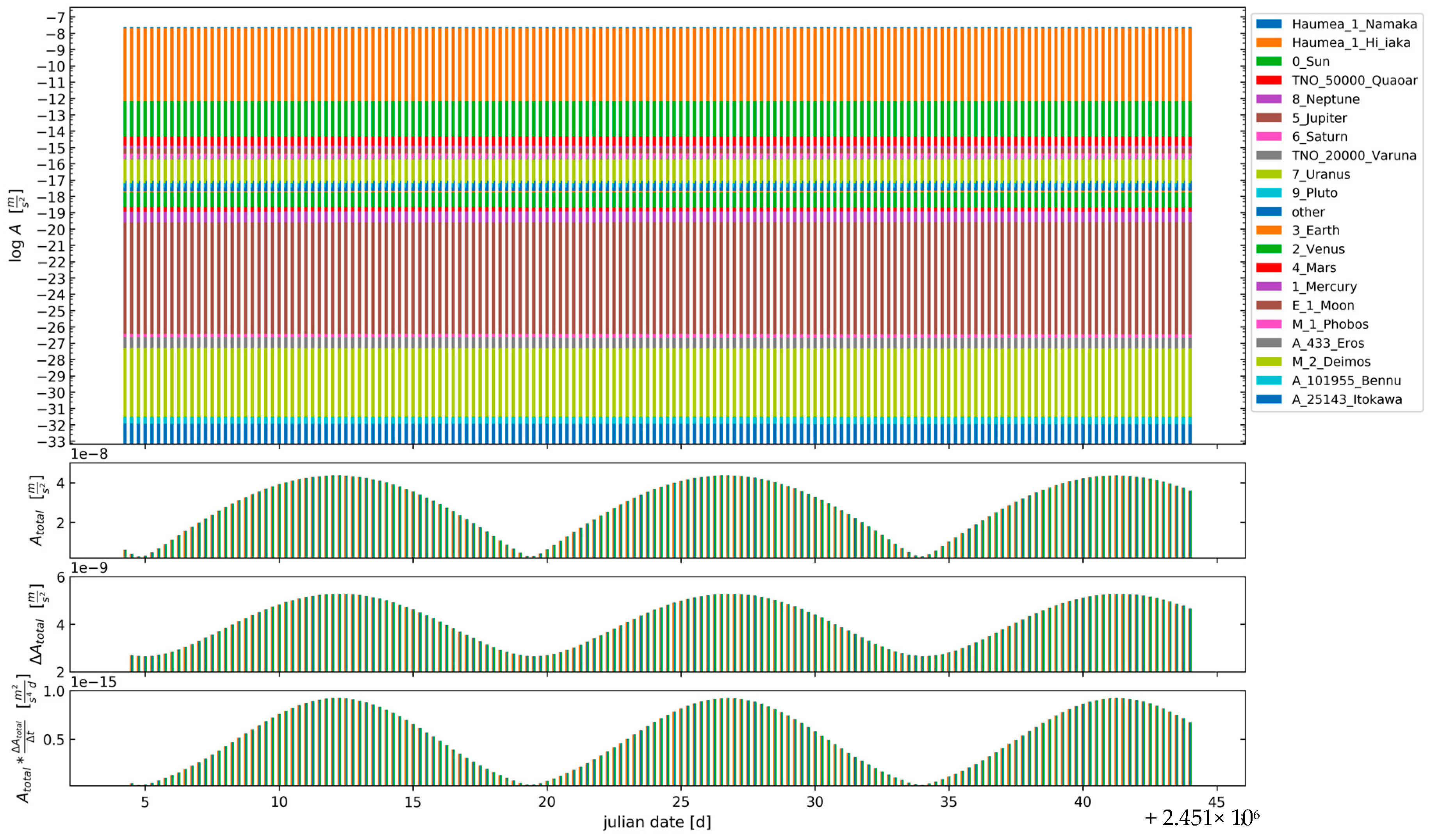
2.1. Tidal Accelerations

Tracking the orbital motion of celestial bodies based on their orbital elements allows the calculation of the positions of the object for discrete time steps and the determination of the three-dimensional distance vectors between the objects. Using a minimalistic set of physical and geometrical parameters of the objects, we calculate the tidal acceleration vectors acting on the surface of one object. After this step, for easier evaluation, the distance vectors were normalized and multiplied by the absolute value of the tidal acceleration A acting on the surface of the influenced object facing the influencing objects following Equation (1).
A = G M r 2 ( 1 ( 1 R r ) 2 1 )
M is the mass of an influencing object; r is the distance between the objects, and R is the radius of the influenced object. Considering also the influences of a changing orbit, we use e (eccentricity), as well as parameters for the orientation of the objects in space and amongst each other, e.g., i (inclination) and Ω (longitude of the ascending node). This allows a computation of acceleration vectors in 3D caused by every object in the system on the investigated one. Adding up these acceleration vectors takes into account that the tidal effects caused by several objects can intensify or partially cancel each other out, due to the different orientations of the tidal acceleration vectors acting on the objects. Determining the vector difference between these “total”, the summed up tidal accelerations for the different time steps also gives a rough estimate of the deformation of the objects and may serve therefore as an indicator for the possible tidal heating on their inside.

2.2. Data

To simulate the motion of the planets, moons, asteroids, and comets in the solar system, one needs the orbital elements of these objects. The data for the planets and their moons are obtained from the Solar System Bodies Archive [7], and the data for the asteroids and comets are gathered from the JPL Small-Body Database Search Engine [8]. Although, being of general importance, masses are only listed for a small fraction of asteroids and comets. To give a rough estimate for the missing masses, we calculate the mean density of the known objects, supplying masses using their radius under the assumption of a spherical shape. Based on this mean density and its standard deviation, an estimate for the masses of the other objects is obtained using their radii. The mean density gives a mean mass estimate, and the mean density plus/minus the standard deviation gives a maximal/minimal mass estimate. With these values, the tidal accelerations for each of the three masses (maximum, mean, and minimum) are computed.
We also include trans-Neptunian objects (TNOs) in our simulation. The data for their physical and orbital properties are taken from various publications listed in the Appendix A in Table A1. For some cases, the given values diverge. We only include TNOs for which the accuracy of the given data seems reasonable: errors of values within a publication <30% or deviations between values of publications <30%. If several value sources for one object were available, we used the mean value of these data. In the column ‘moons’, an asterisk (*) denotes that a moon is known for this TNO but not included in the simulation because of missing or inaccurate data. There are even more multi-body systems, e.g., (42355) Typhon-(42355) Typhon I Echidna. Due to a lack of (unambiguous) data (79360), Sila-Nunam (1997 CS29), (38083) Rhadamanthus (1999 HX11), (15810) Arawn (1994 JR1), (28978) Ixion (2001 KX76), (420356) Praamzius (2012 BX85), (53311) Deucalion (1999 HU11), and many more are not included either. If a value is not given in the publications, the data from the JPL database are used or the mass is derived as mentioned above. The mass and radius of the Sun are taken from [9].
Tidal accelerations are only computed if the radius of the influenced object is larger than 75 km. Since the radius is also part of Equation (1), one also expects low tidal accelerations for these objects. Objects with a radius smaller than 75 km, however, are included in the influencing objects. For comets, we include only the biggest known objects with a radius of around 30 km to test if there could be some tidal potential.
Data used in the simulation of the extrasolar planetary system TRAPPIST-1 are taken for the central star from [10] for mass and radius and for the planets; from [11] for masses, semi-major axes, and eccentricities; from [12] for mean angular motions and radii; and from [6,12] for inclinations.

2.3. Simulation of Orbital Motion

The orbital elements are the semi-major axis a, the eccentricity e, the longitude of the ascending node Ω, the inclination i, the argument of periapsis ω, the mean anomaly at a given epoch M0, and the mean orbital motion n. For the calculation of the three-dimensional distance vectors, the coordinates of all objects have to be transformed into a single Cartesian coordinate system. As the uniform system, the Cartesian heliocentric ecliptic system is chosen with the Sun at the origin and the orbital plane of the Earth as the x-y-plane with the x-axis pointing to the vernal equinox. Kepler’s equation is solved to obtain the polar coordinates of the elliptic orbit; we convert them to Cartesian coordinates and then rotate the orbital plane using the other orbital elements with respect to the ecliptic.
Since the orbital elements of the moons are in reference to their central planet/object, one has to shift their coordinates by those of the central object. The mutual influence of the moons on their orbital motion in the solar system, especially for moons around gas giants, leads to a precession of the orbits and makes it necessary to introduce a new reference plane for some moons, called the Laplace plane. This plane has two additional orbital elements, two angles changing in time, to emulate this precession in a linear approximation. For the outer moons of the gas giants in the solar system, this precession is partly caused by the mutual influence of the outer moons of different planets. Some of the inner moons orbit close to the equatorial plane of their gas giant and therefore use this plane as reference, which also gives two angles as additional orbital elements. Sometimes, these additional angles are in reference to the equatorial plane of the Earth, and one must include an additional rotation about the angle of the obliquity of the Earth.
The code for the simulation written in C++ can be found under the following link: https://www.kip.uni-heidelberg.de/biophysik/software/tidal_accelerations (accessed on 1 July 2021). The need C++11 standard and the library “Eigen” are necessary [13] for compiling.
In order to find an appropriate time window for the simulation of the orbital motion and the resulting tidal accelerations, we choose conjunctions of the planets, since the mutual influence of the moons of different planets, as mentioned above, and therefore the tidal influence should then be maximal. In May 2000, the planets Mercury, Venus, Earth, Mars, Jupiter, and Saturn were located in a relatively small angular segment seen from the Sun. Therefore, it makes sense to simulate around this time point, because the planets are getting very close to each other and may have the highest accelerations on each other. To include the approaching of the planets to this situation, we start our simulation at 1.1.1950, 12 h UT. Around May 2492, almost the same conjunction will occur, so we choose a time period of 600 years for the simulation to include this conjunction as well.
Since one can only simulate for discrete time steps, a reasonable value for each time step has to be determined. For this, we consider the orbital periods of the objects in the solar system. The planets have orbital periods of barely over three months for Mercury to 165 years for Neptune or rather 248 years for the dwarf planet Pluto. In contrast to that, the periods of the moons of the gas giants range from a quarter of a day for the inner ones up to a few years for the outer ones. Among the asteroids, (101955) Bennu orbits in about 1.20 years, while (4) Vesta takes about 3.63 years. TNOs have orbital periods of up to 497.5 years for (90377) Sedna. Comets are strongly diverging, 5.37 years for the Jupiter-family comet 10P/Tempel and 2640 years for (C/1995 O1) Hale-Bopp.
As the asteroids in the main belt have at least a period of about one year, we choose a step size of 90 days in order to have at least four points on the orbit for these asteroids. Additionally, the four inner terrestrial planets, all asteroids, comets, and TNOs, are simulated using this step size, resulting in 600 years/0.25 years = 2400 iterations.
The first interesting moon according to its size is the Saturn moon Mimas with an orbital period of about one day. Again, we choose a quarter of this as our step size and iterate 2400 times, resulting in a total time period of 600 days. In this way, the simulations are carried out for the moons and the terrestrial central objects, Earth, Mars, Pluto, and the TNOs Eris and Haumea, to obtain a more detailed insight into the tidal influence of their moons. To include the conjunction around May 2000, we start the simulation on May 1999 for this smaller step size.
As the orbital periods of the planets in the TRAPPIST-1 system are relatively close to each other with 1.5 to 18.8 days, we chose a smaller step size of 0.1 days. By going for 1800 iterations, we obtain almost 10 orbits for the outermost planet.
Converting the distance vectors into tidal acceleration vectors using Equation (1), we obtain a vector set for every object pointing to the other influencing objects. Since for many celestial bodies, we have three values for the mass (mean, minimal, and maximal guessed mass), we obtain a triple of these tidal accelerations for every time step using these different mass values in calculation, respectively. If the mass is given for an object, we only use this single value so that we end up with identical tidal acceleration vectors instead of different vectors in the triple.
Adding up these vectors related to the influencing objects for a certain time step and taking the norm results in the tidal acceleration Atotal. Note that this takes the three-dimensional orientation of the vectors into account, as the tidal influences of the many objects may (partially) enhance or reduce each other. In addition, we calculate the vector difference of the total acceleration vectors Atotal by subtracting them from each other for two consecutive time steps. We call the norm of this vector difference ΔAtotal. This represents the change of the tidal acceleration vectors, including the change in the orientation. Our idea is that this could give a rough estimation of a deformation of the object caused by the change in the tidal forces.
Equation (1) can be approximated for Rr by
A 2 G M R r 3
Using Δt for the step size in the simulation in days, mean angular motion n, and approximating (ΔA/Δt) by An, we obtain
A Δ A Δ t     A 2 n 4 G 2 M 2 R 2 n r 6
Since parts of the simulation use different step sizes Δt, this product also guarantees the comparability of the values with each other (e.g., moons often complete an orbit faster than a planet).
Please note that for the computation of A and ΔA for each time step in the simulation, as well as the added-up equivalents Atotal and ΔAtotal for each celestial object and their product Atotal·(ΔAtotalt), the full accuracy of Equation (1) is still used. Equation (3) is given to show the variables on the right side (M, R, r, n) the product Atotal·(ΔAtotalt) corresponds to. This might make it easier to compare our results to the viscoelastic models mentioned in the introduction section, e.g., [1,2,3], as one can comprehend how the variables (M, R, r, and n) make up the product Atotal·(ΔAtotalt).
To reduce the amount of resulting data for each object, we apply a pre-screening to find 10 objects with the greatest influence. In addition, we search for 10 objects with the greatest fluctuations in their influence, since this is interesting in connection to the potential for deforming the interior of the celestial body.
To visualize the tidal accelerations, we generate for every object a series of bar charts, applying the values over the discrete time steps. The uppermost graph contains the individual contributions of the influencing objects stacked logarithmically, the second one the resulting Atotal, the third one ΔAtotal, and the last one at the bottom Atotal·(ΔAtotalt). Every bar in these charts consists of three sub-bars, including the value of the tidal acceleration calculated using the minimal, mean, and maximal mass guess from left to right (Figures 1–4, 8–10).
You can find the Python3 script generating the plots using the data resulting from the C++ simulation also in the file package under the above-mentioned link.

3. Results

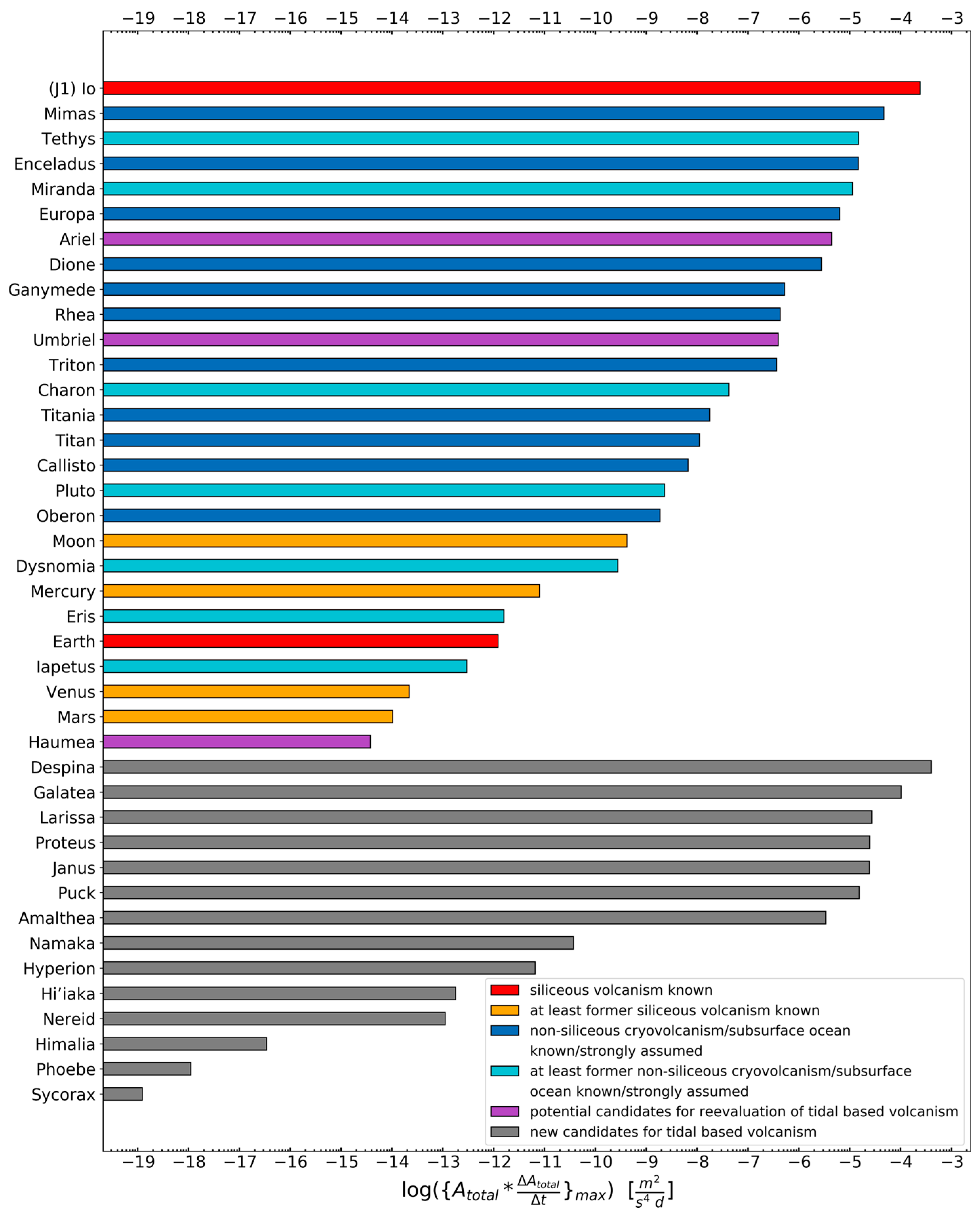
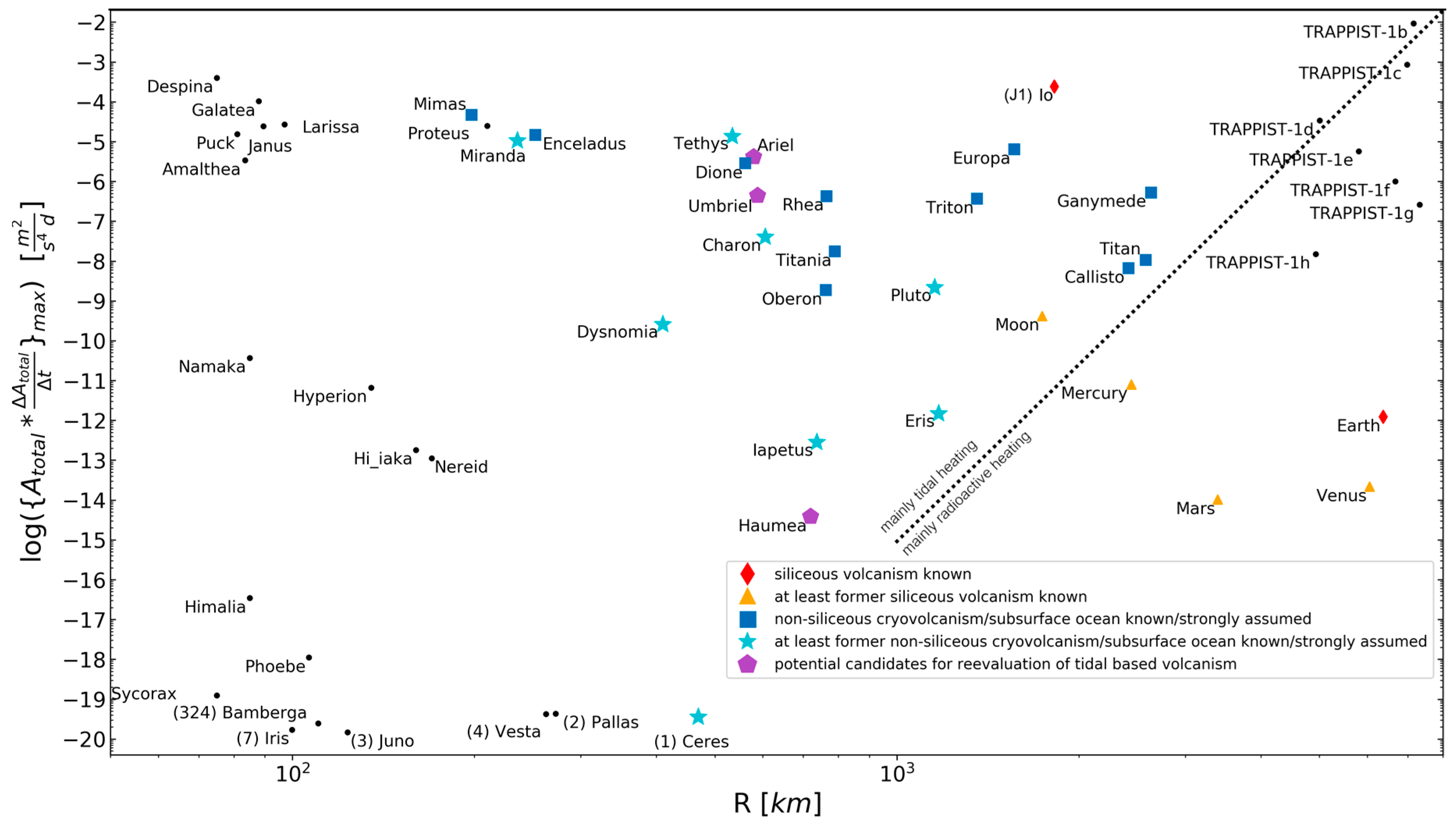
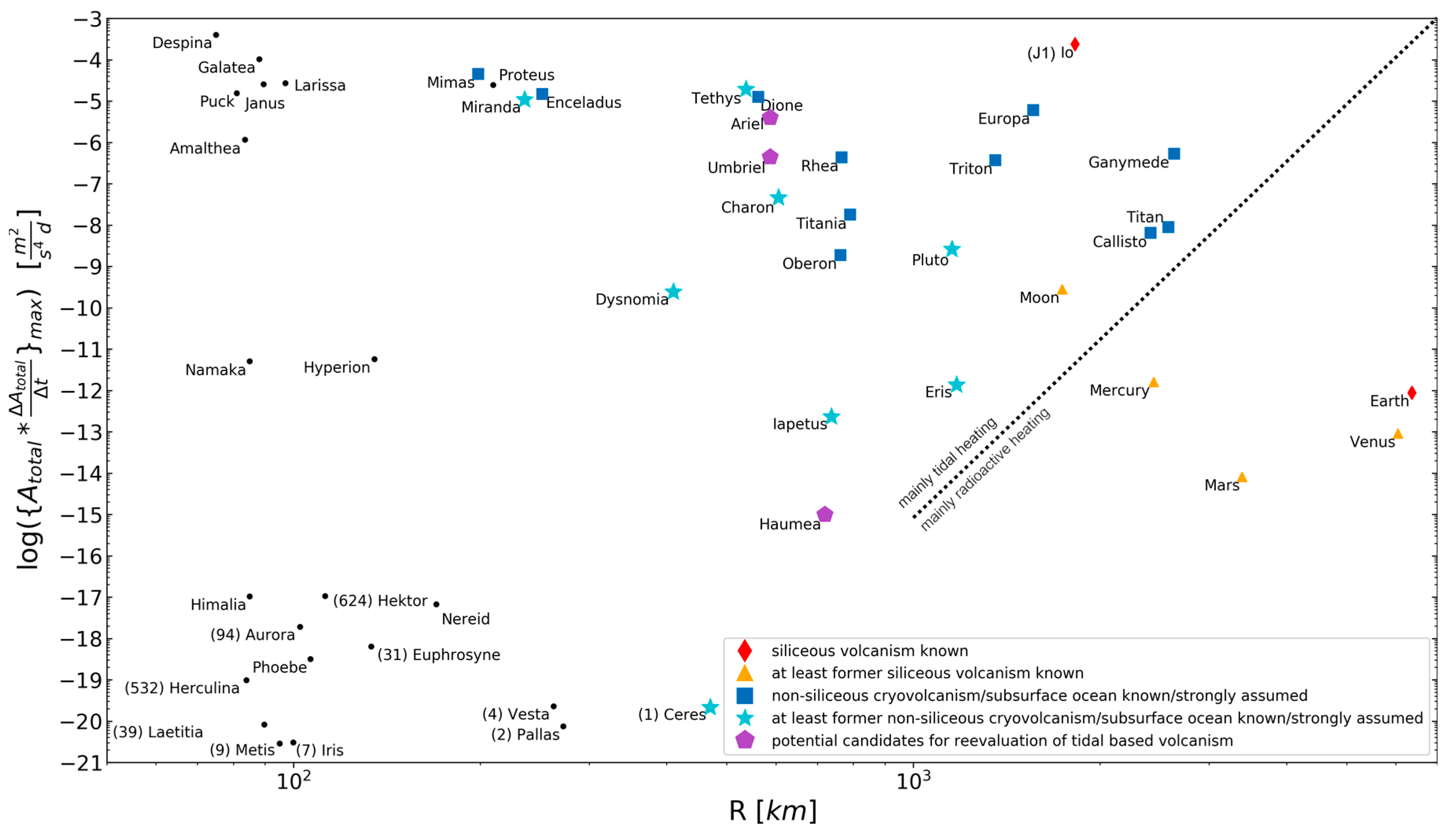
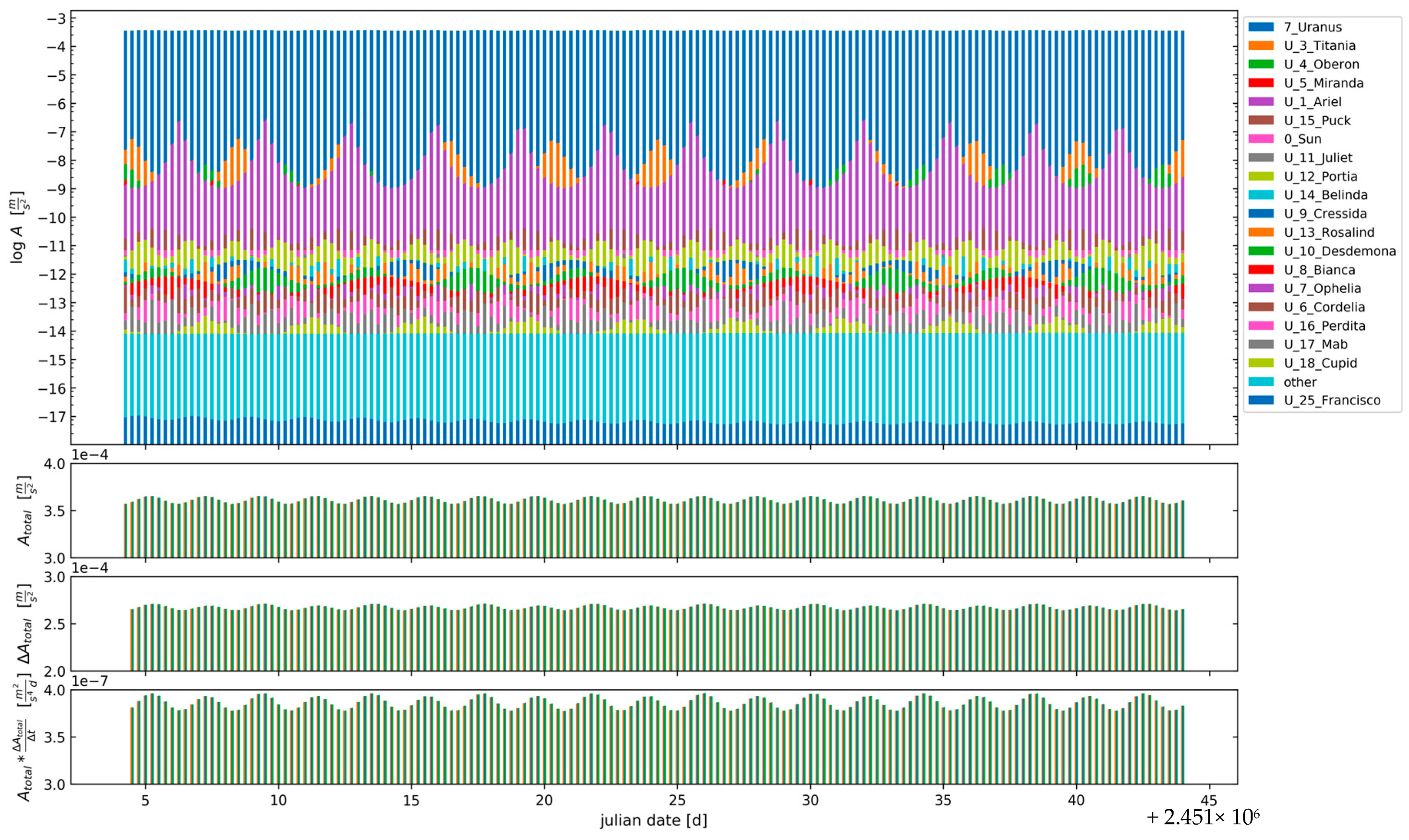
3.1. The Solar System

A typical example is shown in Figure 1, in which all the strongest of the tidal influences acting on the Jovian moon Ganymede can be seen. As expected, Jupiter has the biggest contribution to the tidal acceleration since it is the largest mass around. Second by contribution are the other Galilean moons, but they are already in the range of at least four orders of magnitude smaller. Their periodicities reflect very well the orbital resonances of these moons. Moreover, other Jovian moons appear in the objects causing larger fluctuations than expected. Figure 2 shows as another example the tidal influence acting on (4) Vesta being dominated by the Sun, and its influence is also in the range of three to four orders of magnitude higher than those by planets nearby the main belt and other asteroids within this belt. The results presented in these two figures indicate some general characteristics of our computed tidal accelerations and the expected tidal influences for celestial bodies in our solar system.
Not only the Sun and planets influence (4) Vesta; the Moon and other asteroids such as (1) Ceres, (9) Metis, or (85) Io also generate tidal accelerations that change dramatically over time. Since all these objects including (4) Vesta itself are relatively small, light, and/or too far apart, the absolute values of Atotal·(ΔAtotalt) are too small to be interesting enough in the context of tidal heating. Nevertheless, this shows the potential of asteroids for tidal heating besides moons around large gas giants. One can see in Figure 2 that the course of ΔAtotal follows the course of Atotal in general. This can be explained by the fact that the Sun dominates and ΔAtotal mostly just corresponds to the change of the orientation of Atotal caused by the orbital motion of (4) Vesta around the Sun.
Results for the three-body system Haumea in the Kuiper belt as given in Figure 3 are very interesting in this context, because the orbital planes of the two moons around Haumea are tilted towards each other due to very different inclinations. In this graph (Figure 3), the effect of non-coplanar orbital planes can be nicely seen: The charts showing Atotal and ΔAtotal differ clearly, because the orientations of the tidal acceleration vectors become important in such a tilted system. This contrasts with (4) Vesta as the effects of the moons in the Haumean system are strong enough to dominate ΔAtotal. For objects orbiting close to their central object, it is interesting to check if Atotal and ΔAtotal differ significantly. Objects orbiting close to their central object are often tidally locked, i.e., they are always showing the same side to the central object. In tidal lock, the change in the orientation of the tidal acceleration vector caused by the orbital motion contributes to ΔAtotal, but this alone would not contribute to a deformation of the influenced and tidally locked object over time. If Atotal and ΔAtotal differ, other influences caused by objects other than the central one are contributing, resulting in an actual deformation of the influenced and tidally locked object.
In general, it can be said that among those celestial bodies investigated, TNOs in possession of moons exhibit exceptionally strong tidal influence. In, e.g., [3] a large potential for tidal heating within these TNOs is also described. Multi-body TNO systems often consist of relatively large objects orbiting each other in short distance and have, in comparison with solar system planets and moons, quite uncommon values for their orbital elements. Nevertheless, as the accuracy or availability of orbital and physical data for TNOs are in general not very satisfying, especially for TNOs with moons, a (more precise) determination of these parameters could be very interesting for a more detailed evaluation of tidal heating.
As the model gives a complete three-dimensional simulation evolving over time, rare and only occasionally occurring encounters of generally not-associated objects are more easily revealed. This is especially interesting for comets and some asteroids that travel across the inner and outer regions of the solar system due to their high eccentricities. In Figure 4, the flyby of the comet C/1995 O1 (Hale-Bopp) past Jupiter is shown. The tidal influence increases significantly as Hale-Bopp approaches Jupiter. The tidal accelerations are nevertheless small, and the considered parameters are many orders of magnitude below those of objects shown above. This may be mainly due to the small size of Hale-Bopp but could become interesting for bigger asteroids or comets.
Figure 5 gives an overview of the celestial bodies showing the largest tidal accelerations in the solar system. {Atotal·(ΔAtotalt)}max is the maximal value found for the celestial object over all time steps.
In Figure 6 and Figure 7, the volcanism of differently sized objects is discussed in relation to the maximal value {Atotal·(ΔAtotalt)}max. Celestial bodies marked by orange triangles show signs of at least former volcanism, meaning that these objects certainly had volcanism in the past and might even be faintly igneous today. Data of the space probe MESSENGER shows signs of siliceous flood volcanism and other volcanic features on Mercury [14,15]. Venus shows multiple signs for former and maybe still present volcanism. The Monitoring Camera of the space probe Venus Express [16], numerical simulations [17], and other investigations [18,19,20] find hints/evidence for volcanism. It is reasonably certain that Mars used to be volcanic in the past (e.g., Olympus Mons) and maybe still is today. Additionally, our Moon shows signs of former volcanism [21], and seismic measurements during the Apollo missions indicate present volcanism [22]. This subgroup is presented just for orientation, as one must consider for these huge objects that radioactive heating and stored accretion energy strongly contribute along with tidal interactions to volcanism.
As may be already seen from Figure 6, if {Atotal·(ΔAtotalt)}max is larger than 10−15 (m2/s4d) and R larger than 200 km, volcanism is known for all objects in the solar system. This general observation makes no assumptions on the power sources of this volcanism. For larger R, this may be more based on radioactive decay or stored accretion energy; for smaller R, this points more toward the direction of tidal heating. This is indicated approximately by the dashed line in Figure 6 and Figure 7 and was determined empirically by considering the volcanic activities of the objects in the solar system. Nevertheless, this boundary remains blurred and should not be considered too certain. Most planets with at least former volcanism known are below 10−10 (m2/s4d) and above 10−15 (m2/s4d) but have higher R values. The probably most interesting new objects exposed to higher gravitational forces found by this simulation can be seen in the upper left corner of the diagram with {Atotal·(ΔAtotalt)}max larger than 10−6 (m2/s4d) but R smaller than 200 km. New considerations may also be taken for all other objects shown, even if they are not inside of the boundaries as the objects already described.
As mentioned above, for objects in extrasolar planetary systems, very often only a small fraction of their properties and parameters is available. Even orbital elements may be missing or vague. Thus, the application of our simulations is running into uncertainties. To investigate the effect of neglecting some orbital elements on the results of our model, we repeated our whole full simulation by setting e, Ω, i, ω, and M0 to zero so that only a, n, M, and R were remaining, which often may be the only well-known parameters for objects in an extrasolar planetary system. The new results based on this simplified simulation are given in Figure 7. Only small deviations were found between the two versions (Figure 7 vs. Figure 6) of the simulation. This may be mostly caused by neglecting the eccentricity e (as been seen in pre-simulations when testing the algorithm, data not shown). The similarity of Figure 6 and Figure 7 shows that the simplified version of the simulation with a smaller set of orbital elements does not change the resulting tidal accelerations significantly. Thus, the simplified version could be very applicable to estimate the potential significance of tidal influences in extrasolar planetary systems, especially the ones with poorly known or many unknown orbital elements. In general, the deviations are reasonably small, and therefore our approach may be considered stable enough to provide an estimate for the tidal interaction and the heating potential in extrasolar planetary systems, even if not all parameters are known. An example is given in Figure 8 for Haumea, where even with strong influences from its orbital planes, the course of the values changes, thereby remaining in the same order of magnitude (in comparison to Figure 3).
In the case of special objects where uncertainties are present, the bar histograms of tidal accelerations may give new insights for future improved modeling. As an example of the solar system, the two Uranian moons Ariel and Umbriel are shown. Little energy transfer from their central planet is assumed, but periodic mutual tidal influences of the moons seem to peak over 10−7 m/s2 for Atotal nearly all three days (Figure 9). This shows that also other objects orbiting the central object can provide the leading important tidal influence. This is a key new feature of the model presented here. We can see (e.g., bottom panel of Figure 9) that referring all calculations to the central object only might underestimate the potential of tidal influences by other objects present in the system. This example may justify our complex multi-body approach in the case of special planetary systems.

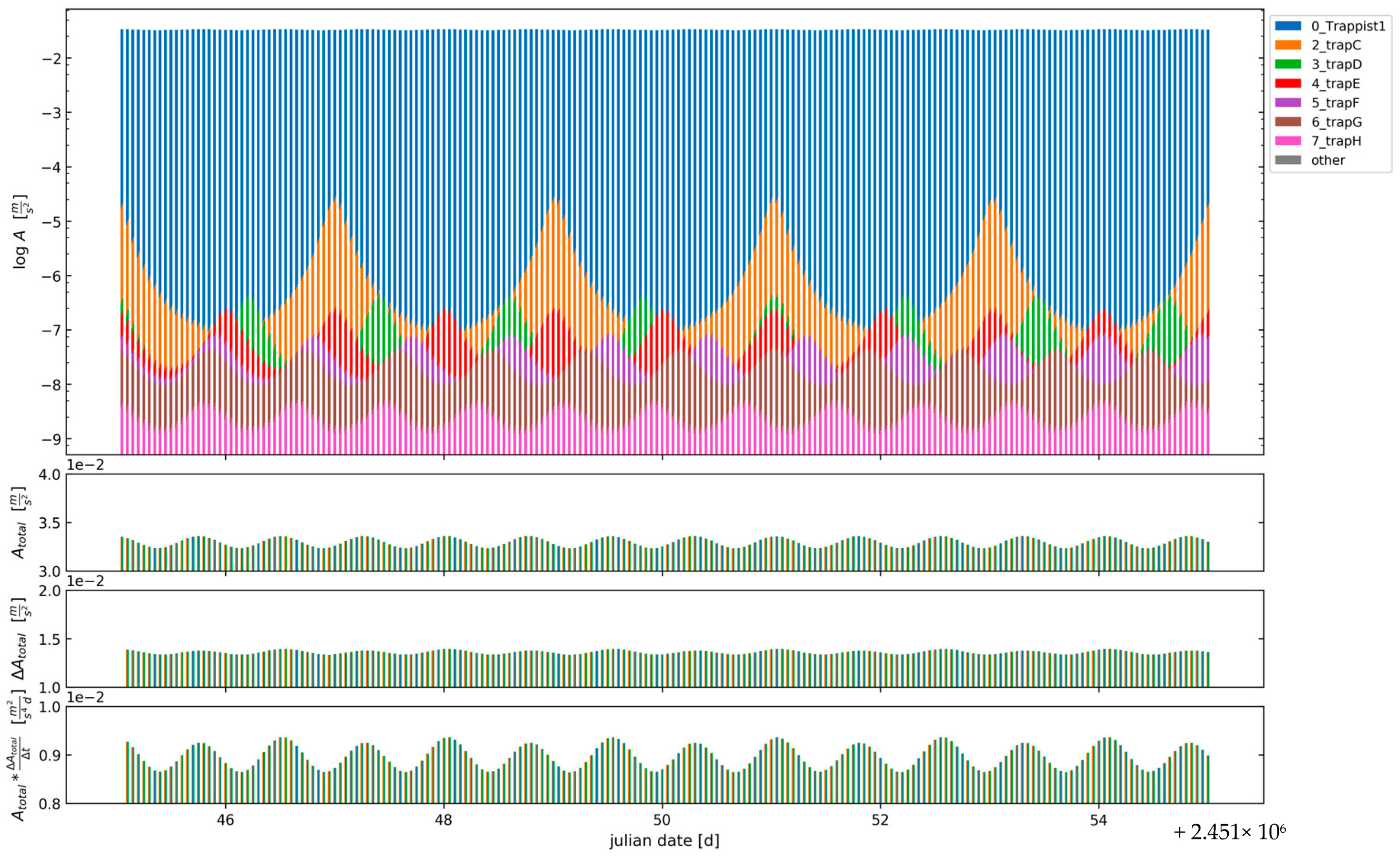
3.2. Extrasolar Planetary System TRAPPIST-1

A well-investigated extrasolar planetary system is TRAPPIST-1, an M-dwarf with seven exoplanets [5,6], the largest extrasolar planetary system of terrestrial Earth-sized planets found so far. Since all planets are orbiting very close to each other and their host star, this system is of great interest and a challenging example for our approach concerning tidal interactions and consequences, especially for tidal heating.
What distinguishes this system from all others is that the masses, semi-major axes, eccentricities, mean angular motions, radii, and inclinations are known with high accuracy, and this, quite remarkably, for all the seven terrestrial Earth-sized planets [6,11,12]. The central star is an ultra-cold red dwarf star [6,10] of spectral type M8V, with a size slightly larger than Jupiter, but 94 times Jupiter’s mass, which is located 12 pc (about 41 light-years) away from the Sun [35].
There are extensive studies elaborating on the possible habitability of this system. Considerations about the equilibrium temperatures based on the irradiation by the host star [12] could allow for liquid water on the surfaces of up to six planets (TRAPPIST-1c, -d, -e, -f, -g, and -h) when assuming a very optimistic circumstellar habitable zone around the host star, or up to three planets (TRAPPIST-1e, -f, and -g), when assuming a conservative circumstellar habitable zone, depending on definition, see, e.g., [36,37,38,39], among many others. The models in [40,41], considering the potential water loss from terrestrial planets around ultra-cold red dwarf stars during their pre-main sequence phase, conclude for the TRAPPIST-1 planets -b and -c that they may have lost as much as 15 Earth oceans of water; -g may have lost more than 20 Earth oceans and -e less than 3 Earth oceans of water. For TRAPPIST-1d, they predict a water loss of possibly less than one Earth ocean. Depending on the initial water content of these planets, they could have enough water to remain habitable when they enter the habitable zone in the main sequence phase of their host star TRAPPIST-1. The elaborate climate model in [42] predicts that TRAPPIST-1e has the highest probability for being an Earth-like ocean world.
Figure 10 shows tidal accelerations for the innermost planet TRAPPIST-1b, which even exceed the values found for the Jovian moon (J1) Io, the most strongly tidally influenced object in the solar system. Equally, the planets on outer orbits show values in the same range (not shown). We may therefore assume strong to very strong tidal heating, and consequently siliceous volcanism may be present if we refer to the relations of Figure 6. This is in good agreement with results in other publications, e.g., [43], confirming an applicability of our model to extrasolar planetary systems. Additionally, the individual tidal influences of all other planets are also visible. The influence of TRAPPIST-1c alone would be enough to periodically exert tidal forces on TRAPPIST-1b up to a lower limit from which on tidal heating of low-melting liquids might already be considered. As M-dwarfs often possess extremely strong magnetic fields, another source for heat induction has to be considered [44]. Adding up stored accretion energy, radioactive, tidal, and induction heating, this gives an impression of the planets of TRAPPIST-1 as volcanic worlds. An overview and classification in relation to objects in the solar system is given in Figure 6.
For better comparison, we calculate the values of {Atotal·(ΔAtotalt)}max found in our model using full parameters for (J1) Io, Ganymede, and all planets in the TRAPPIST-1 system (Table 1). We choose (J1) Io and Ganymede because their semi-major axes a are similar to the ones of the planets in the TRAPPIST-1 system and Jupiter as the object being orbited by (J1) Io and Ganymede is with its huge mass most comparable to the M-dwarf.

4. Discussion

As a “gold standard” system, the simulation approach for tidal accelerations presented here using a minimalistic set of parameters was applied to all objects in our solar system known and correlated to cryo- or even siliceous volcanism. For celestial bodies known to show signs of strong tidal influence, the resulting values for {Atotal·(ΔAtotalt)}max are among the largest occurring in this simulation. Furthermore, additional objects were suggested, which have not been subjects of research for tidal heating up to now.
The identification of new candidates can also reveal conclusions about the composition and evolution of other properties not related to tidal heating, e.g., the inner Neptunian moon Despina shows the highest tidal acceleration value of all objects included in the simulation of the solar system (see Figure 5 and Figure 6). According to [45], the composition of Despina and the other inner Neptunian moons should be structured like a rubble pile, i.e., a loose aggregation of small rocky pieces. Considering the strong tidal forces presumably associated with the relatively high tidal accelerations acting on Despina, it may be interesting to investigate whether or even how rubble piles exposed to such relative strong tidal forces are stable over the long history of the solar system. Therefore, this could lead to new insights into the stability of rubble piles or motivate new ideas about the inner composition of these objects.
As may have been noticed in Figure 5, the Earth shows siliceous volcanism, although the tidal accelerations are quite low compared to (J1) Io, the only other object in the solar system for which this persistent characteristic is confirmed. This can be explained by the fact that due to the large radius of Earth, accretion heat from the period of formation and radioactive heating contribute more to the occurrence of volcanism on Earth than tidal heating. This also illustrates the need for awareness and consideration of other influences not covered just by tidal acceleration or tidal heating. Nevertheless, this is not a contradiction to our approach. In Figure 6 and Figure 7, one can easily distinguish two main domains (indicated approximately by the dashed line): big objects like our Earth appear at the far-right margin of the plots at large radii R, implying large contributions from radioactive decay and stored accretion energy. The other domain is tidally interesting objects, appearing at the top in the center and the left margin of the plots with small to intermediate radii R but large tidal accelerations. Therefore, this domain is the interesting one for tidal heating as the main contribution. Accretion heat and radioactive heating should be minor. All the objects considered as interesting ones in our study for the solar system can be found in this domain. It can be divided into two sub-domains: The top center contains the already well-known objects in the context of (cryo-)volcanism and tidal heating. The top left corner contains the additional objects suggested in this study, which have not been subjects of research for tidal heating until now.
When looking at Figure 6 and Figure 7, generalized boundaries for where cryo- and siliceous volcanism might be expected for a celestial object based on our solar system may not easily be transferred to extrasolar planetary systems. The smaller the extrasolar objects are (small radii R below the size of Earth), the easier this is to perform, as then mainly tidal forces should dominate the potential volcanic activity on these worlds.
Approximate boundaries based on our solar system might be given to estimate the tidal-dominated volcanic activity on small extrasolar objects in future studies: The before mentioned minimal values of 10−15 (m2/s4d) for {Atotal·(ΔAtotalt)}max and 200 km for R should hint at possible cryovolcanic activity when found in an extrasolar planetary system. The lower bound for potential siliceous volcanism powered by tidal influences might be deduced by the order of magnitude of the value of {Atotal·(ΔAtotalt)}max for (J1) Io, roughly about 10−4 (m2/s4d) (compare to Table 1). These boundaries may be transferable to sub-Earth-sized extrasolar objects, as potential volcanic processes in these small worlds might clearly be tidal-dominated.
For larger extrasolar objects, the two other influences on the volcanic activity mentioned, radioactive decay and stored accretion energy, have to be considered. Both may not be easily modeled when transferring to extrasolar systems of Earth’s size and larger. A main reason for that may be the decline of these influences over time. This can already be seen in our solar system, as, e.g., Mars shows signs of mostly extinct volcanism that may mainly be dominated by radioactive decay and stored accretion energy.
The larger R, the better internal models considering the remaining accretion energy stored from the object’s formation have to be. Additionally, for radioactive heating, other parameters and events have to be considered. These are mainly the metallicity of the host star, uneven distributions of these (radioactive) metals during planetary formation, possible special external metal enrichment events, or other special events shortly after the planet’s formation. Examples in the solar system are the potential enrichment of the radioactive aluminum isotope 26Al in the solar nebula by external sources [46,47] and the potential giant collision between the proto-Earth and a planetary embryo named Theia forming the Moon and having consequences for the composition of both the Earth and the Moon, see, e.g., [48].
Detailed and thorough analyses have to be performed for large R when trying to transfer the boundaries for expected volcanism given above from the solar to extrasolar systems. The older and the less enriched in radioactive metals the extrasolar system is, and the smaller the exoplanets(/-moons) are, the more reliable this transfer via our approach may be.
The dashed line in Figure 6 and Figure 7 shows via empirical findings in our solar system the division line for tidal-dominated and radioactive decay/stored accretion-energy-dominated objects. Again, the transfer of this division to extrasolar systems has to be performed cautiously due to the issues outlined above. This division line remains blurred and should not be considered too certain.
As a first interpretation, this may be performed for the extrasolar planetary system TRAPPIST-1. The host star TRAPPIST-1 has a metallicity close to our Sun [12]. The age of this system might be older than our solar system [49]. This might favor a dominant influence by tidal heating in the present phase of this system, as the other possible energy sources might have dwindled further. Planets in the TRAPPIST-1 system have been taken to test and verify but also to show the limits and borders of this model. The objects are already quite big in comparison with considered objects in the solar system, but they are until now the only set of exoplanets well-characterized enough by other models to serve as check-up for our model. Planets of TRAPPIST-1 should experience strong heating by remaining accretion heat, radioactive heating, and tidal heating all together, as they appear close to the dashed line in Figure 6. Hence, planets of TRAPPIST-1 appear to be very hot worlds. This is in concordance with the conclusions from other simulations [43,50,51].
Future investigations might try to apply this simulation approach to depict perturbations regarding ΔA. It may be an aim to make long-term predictions about the stability and resonances of multi-body systems, since the mutual perturbations of the objects in an energetically relaxed state are visible (energy included in eccentricities dissipated to zero).
Furthermore, simulations without the central object might be desirable to investigate only the mutual tidal influences of the orbiting objects. As already mentioned, this will show that also other objects orbiting the central object can provide the leading important tidal influence (see, e.g., the bottom panel of Figure 9 for Umbriel). This may justify our complex multi-body approach.
Some new objects of interest were found and may justify further investigations. The testing of how strong the values change when some parameters are missing yields stable/similar results in the solar system. This encourages the application in extrasolar planetary system to evaluate less well-known objects. The transfer to the extrasolar planetary system TRAPPIST-1 also results in assumptions of the planets being in concordance with known simulations [43,50,51]. This confirms our choice of TRAPPIST-1 for verification that our model is applicable to extrasolar planetary systems. It might be encouraging to use this approach on further extrasolar systems.
Only few sub-Earth-sized exoplanets with accurately measured physical and orbital parameters are known today. Among others, an outstanding example for such an extrasolar system of terrestrial and sub-Earth-sized planets is Kepler-444, an old triple-star system with five planets orbiting around the main star (K type) [52]. Nevertheless, not for all planets, and only few parameters are known in this system. We are eagerly waiting for the first observations by the upcoming James Webb Space Telescope, which should provide new and more accurate measurements of physical and orbital parameters of extrasolar planetary systems, in particular, as well for sub-Earth-sized exoplanets. Many “super-Earth” systems were found already, e.g., HD 10180 [53], LHS 1140 [54], and many others. As the TRAPPIST-1 system contains planets larger than Earth, we hope that it allows us to extend our parameter space and that it might serve as the link to these larger worlds. Nevertheless, the mentioned issues regarding the reliability of possible future finding with our model have to be carefully addressed to select appropriate tidal-dominated larger worlds applicable for our approach in future studies. So-called “mini-Neptunes”, e.g., Kepler-11f [55], Kepler-138d [56,57], and others, could be interesting as well. In a follow-up study, we plan to apply our model to these and other extrasolar systems.

Author Contributions

Conceptualization, G.H.; methodology, K.P. and G.H.; software, K.P.; validation, K.P., A.R., and G.H.; formal analysis, K.P.; investigation, K.P., A.R., and G.H.; resources, M.H. and G.H.; data curation, K.P.; writing—original draft preparation, K.P.; writing—review and editing, A.R., M.H., and G.H.; visualization, K.P.; supervision, M.H. and G.H. All authors have read and agreed to the published version of the manuscript.

Funding

This research received no external funding.

Institutional Review Board Statement

Not applicable.

Informed Consent Statement

Not applicable.

Data Availability Statement

Acknowledgments

The authors thank Margot Chazotte, Aaron Sievers, Andrea Zanna, and Silvia Zanna for stylistic review of the manuscript.

Conflicts of Interest

The authors declare no conflict of interest.

Appendix A

This appendix contains details and resources of data.
Table A1. Resources of data for TNOs. If several value sources for one object were available, we used the mean value of these data. In the column ‘moons’, an asterisk (*) denotes that a moon is known for this TNO but not included in the simulation because of missing or inaccurate data.
TNORadiusMassOrbital ElementsMoons
(19521) Chaos (1998 WH24)[58]
(38628) Huya (2000 EB173)[58]
(47171) Lempo (1999 TC36)[58][59]
(50000) Quaoar (2002 LM60)[58,60][60,61] *
(58534) Logos (1997 CQ29)[62][62] *
(65489) Ceto (2003 FX128)[58][63] *
(66652) Borasisi (1999 RZ253)[58][64] *
(88611) Teharonhiawako (2001 QT297)[58][64] *
(90377) Sedna (2003 VB12)[58]
(90482) Orcus (2004 DW)[58][65] *
(120347) Salacia (2004 SB60)[58][58,66] *
(136108) Haumea[58,67,68] Namaka, Hi’iaka
(136199) Eris (2003 UB313)[69][70] Dysnomia
(136472) Makemake (2005 FY9)[68,71] *
(148780) Altjira (2001 UQ18)[58][58]
(174567) Varda (2003 MW12)[58][72] *
(136108) Haumea II Namaka[3][3][67]
(136108) Haumea I Hi’iaka[3][3][67]
(136199) Eris I Dysnomia[3][3][70]

References

  1. Peale, S.J.; Cassen, P.; Reynolds, R.T. Melting of Io by tidal dissipation. Science 1979, 203, 892–894. [Google Scholar] [CrossRef] [Green Version]
  2. Meyer, J.; Wisdom, J. Tidal heating in Enceladus. Icarus 2007, 188, 535–539. [Google Scholar] [CrossRef] [Green Version]
  3. Saxena, P.; Renaud, J.P.; Henning, W.G.; Jutzi, M.; Hurforda, T. Relevance of tidal heating on large TNOs. Icarus 2018, 302, 245–260. [Google Scholar] [CrossRef] [Green Version]
  4. Dressing, C.D.; Charbonneau, D. The occurrence rate of small planets around small stars. Astrophys. J. 2013, 767, 95. [Google Scholar] [CrossRef] [Green Version]
  5. Gillon, M.; Jehin, E.; Lederer, S.M.; Delrez, L.; de Wit, J.; Burdanov, A.; van Grootel, V.; Burgasser, A.J.; Triaud, A.H.M.J.; Opitom, C.; et al. Temperate Earth-sized planets transiting a nearby ultracool dwarf star. Nature 2016, 533, 221–224. [Google Scholar] [CrossRef] [PubMed] [Green Version]
  6. Gillon, M.; Triaud, A.H.M.J.; Demory, B.O.; Jehin, E.; Agol, E.; Deck, K.M.; Lederer, S.M.; de Wit, J.; Burdanov, A.; Ingalls, J.G.; et al. Seven temperate terrestrial planets around the nearby ultracool dwarf star TRAPPIST-1. Nature 2017, 542, 456–460. [Google Scholar] [CrossRef] [PubMed]
  7. Solar System Bodies; Jet Propulsion Laboratory (JPL), California Institute of Technology (Caltech) and National Araeronatics and Space Agengy (NASA): Pasadena, CA, USA, 1996. Available online: https://ssd.jpl.nasa.gov/?bodies (accessed on 13 February 2018).
  8. JPL Small-Body Database Search Engine; Jet Propulsion Laboratory (JPL), California Institute of Technology (Caltech) and National Araeronatics and Space Agengy (NASA): Pasadena, CA, USA, 1996. Available online: https://ssd.jpl.nasa.gov/sbdb_query.cgi (accessed on 13 February 2018).
  9. Steadly, R.S.; Robinson, M.S. The Astronomical Almanac for the Year 2012: Data for Astronomy, Space Sciences, Geodesy, Surveying, Navigation and other Applications; U.S. Government Printing Office: St. Louis, MO, USA, 2011; ISBN 978-0-7077-41215.
  10. Van Grootel, V.; Fernandes, C.S.; Gillon, M.; Jehin, E.; Manfroid, J.; Scuflaire, R.; Burgasser, A.J.; Barkaoui, K.; Benkhaldoun, Z.; Burdanov, A.; et al. Stellar parameters for Trappist-1. Astrophys. J. 2018, 853, 30. [Google Scholar] [CrossRef] [Green Version]
  11. Grimm, S.L.; Demory, B.-O.; Gillon, M.; Dorn, C.; Agol, E.; Burdanov, A.; Delrez, L.; Sestovic, M.; Triaud, A.H.M.J.; Turbet, M.; et al. The nature of the TRAPPIST-1 exoplanets. Astron. Astrophys. 2018, 613, A68. [Google Scholar] [CrossRef]
  12. Delrez, L.; Gillon, M.; Triaud, A.H.M.J.; Demory, B.-O.; de Wit, J.; Ingalls, J.G.; Agol, E.; Bolmont, E.; Burdanov, A.; Burgasser, A.J.; et al. Early 2017 observations of TRAPPIST-1 with Spitzer. Mon. Not. R. Astron. Soc. 2018, 475, 3577–3597. [Google Scholar] [CrossRef]
  13. Guennebaud, G.; Jacob, B. Eigen v3 [C++ library]. 2010. Available online: http://eigen.tuxfamily.org (accessed on 13 February 2018).
  14. Hanson, B. Mercury, up-close again. Introduction. Science 2008, 321, 58. [Google Scholar] [CrossRef] [Green Version]
  15. Head, J.W.; Chapman, C.R.; Strom, R.G.; Fassett, C.I.; Denevi, B.W.; Blewett, D.T.; Ernst, C.M.; Watters, T.R.; Solomon, S.C.; Murchie, S.L.; et al. Flood volcanism in the northern high latitudes of Mercury revealed by MESSENGER. Science 2011, 333, 1853–1856. [Google Scholar] [CrossRef] [Green Version]
  16. Shalygin, E.V.; Markiewicz, W.J.; Basilevsky, A.T.; Titov, D.V.; Ignatiev, N.I.; Head, J.W. Active volcanism on Venus in the Ganiki Chasma rift zone. Geophys. Res. Lett. 2015, 42, 4762–4769. [Google Scholar] [CrossRef]
  17. Armann, M.; Tackley, P.J. Simulating the thermochemical magmatic and tectonic evolution of Venus’s mantle and lithosphere: Two-dimensional models. J. Geophys. Res. Planets 2012, 117, E12003. [Google Scholar] [CrossRef] [Green Version]
  18. Ulmschneider, P. Intelligent Life in the Universe: Principles and Requirements Behind Its Emergence, 2nd ed.; Springer: Berlin/Heidelberg, Germany, 2006; ISBN 978-3-540-32836-0. [Google Scholar]
  19. Scholz, M. Astrobiologie; Springer Spektrum: Berlin/Heidelberg, Germany, 2016; ISBN 978-3-662-47036-7. [Google Scholar]
  20. Mikhail, S.; Heap, M.J. Hot climate inhibits volcanism on Venus: Constraints from rock deformation experiments and argon isotope geochemistry. Phys. Earth Planet. Inter. 2017, 268, 18–34. [Google Scholar] [CrossRef] [Green Version]
  21. Spudis, P.D. Volcanism on the Moon. In The Encyclopedia of Volcanoes, 2nd ed.; Sigurdsson, H., Houghton, B., McNutt, S., Rymer, H., Stix, J., Eds.; Academic Press: London, UK, 2015; Volume 39, pp. 689–700. ISBN 978-0-12-385938-9. [Google Scholar]
  22. Weber, R.C.; Lin, P.-Y.; Garnero, E.J.; Williams, Q.; Lognonné, P. Seismic detection of the lunar core. Science 2011, 331, 309–312. [Google Scholar] [CrossRef] [Green Version]
  23. Anderson, J.D.; Schubert, G.; Jacobson, R.A.; Lau, E.L.; Moore, W.B.; Sjogren, W.L. Europa’s differentiated internal structure: Inferences from four Galileo encounters. Science 1998, 281, 2019–2022. [Google Scholar] [CrossRef]
  24. Vance, S.; Bouffard, M.; Choukroun, M.; Sotin, C. Ganymede׳s internal structure including thermodynamics of magnesium sulfate oceans in contact with ice. Planet. Space Sci. 2014, 96, 62–70. [Google Scholar] [CrossRef]
  25. Showman, A.P.; Malhotra, R. The Galilean satellites. Science 1999, 286, 77–84. [Google Scholar] [CrossRef] [Green Version]
  26. Hansen, C.J.; Esposito, L.; Stewart, A.I.F.; Colwell, J.; Hendrix, A.; Pryor, W.; Shemansky, D.; West, R. Enceladus’ water vapor plume. Science 2006, 311, 1422–1425. [Google Scholar] [CrossRef] [PubMed] [Green Version]
  27. Grasset, O.; Sotin, C.; Deschamps, F. On the internal structure and dynamics of Titan. Planet. Space Sci. 2000, 48, 617–636. [Google Scholar] [CrossRef]
  28. Beuthe, M.; Rivoldini, A.; Trinh, A. Enceladus’s and Dione’s floating ice shells supported by minimum stress isostasy. Geophys. Res. Lett. 2016, 43, 10088–10096. [Google Scholar] [CrossRef] [Green Version]
  29. Hussmann, H.; Sohl, F.; Spohn, T. Subsurface oceans and deep interiors of medium-sized outer planet satellites and large trans-neptunian objects. Icarus 2006, 185, 258–273. [Google Scholar] [CrossRef]
  30. Tittemore, W.C.; Wisdom, J. Tidal evolution of the Uranian satellites: III. Evolution through the Miranda-Umbriel 3:1, Miranda-Ariel 5:3, and Ariel-Umbriel 2:1 mean-motion commensurabilities. Icarus 1990, 85, 394–443. [Google Scholar] [CrossRef]
  31. Bergstralh, J.T.; Miner, E.D.; Matthews, M.S. Uranus; The University of Arizona Press: Tucson, AZ, USA, 1991; ISBN 0-8165-1208-6. [Google Scholar]
  32. Ruesch, O.; Platz, T.; Schenk, P.; McFadden, L.A.; Castillo-Rogez, J.C.; Quick, L.C.; Byrne, S.; Preusker, F.; O’Brien, D.P.; Schmedemann, N.; et al. Cryovolcanism on Ceres. Science 2016, 353, aaf4286. [Google Scholar] [CrossRef] [Green Version]
  33. Desch, S.J.; Cook, J.C.; Doggetta, T.C.; Portera, S.B. Thermal evolution of Kuiper belt objects, with implications for cryovolcanism. Icarus 2009, 202, 694–714. [Google Scholar] [CrossRef]
  34. Dumas, C.; Carry, B.; Hestroffer, D.; Merlin, F. High-contrast observations of (136108) Haumea. Astron. Astrophys. 2011, 528, A105. [Google Scholar] [CrossRef] [Green Version]
  35. Costa, E.; Méndez, R.A.; Jao, W.-C.; Henry, T.J.; Subasavage, J.P.; Ianna, P.A. The solar neighborhood. XVI. Parallaxes from CTIOPI: Final results from the 1.5 m Telescope Program. Astron. J. 2006, 132, 1234–1247. [Google Scholar] [CrossRef] [Green Version]
  36. Kasting, J.F.; Whitmire, D.P.; Reynolds, R.T. Habitable zones around main sequence stars. Icarus 1993, 101, 108–128. [Google Scholar] [CrossRef]
  37. Selsis, F.; Kasting, J.F.; Levrard, B.; Paillet, J.; Ribas, I.; Delfosse, X. Habitable planets around the star Gliese 581? Astron. Astrophys. 2007, 476, 1373–1387. [Google Scholar] [CrossRef] [Green Version]
  38. Kane, S.R.; Gelino, D.M. The habitable zone gallery. Publ. Astron. Soc. Pac. 2012, 124, 323–328. [Google Scholar] [CrossRef] [Green Version]
  39. Kopparapu, R.K. A revised estimate of the occurrence rate of terrestrial planets in the habitable zones around Kepler M-dwarfs. Astrophys. J. Lett. 2013, 767, L8. [Google Scholar] [CrossRef] [Green Version]
  40. Bolmont, E.; Selsis, F.; Owen, J.E.; Ribas, I.; Raymond, S.N.; Leconte, J.; Gillon, M. Water loss from terrestrial planets orbiting ultracool dwarfs: Implications for the planets of TRAPPIST-1. Mon. Not. R. Astron. Soc. 2017, 464, 3728–3741. [Google Scholar] [CrossRef] [Green Version]
  41. Bourrier, V.; de Wit, J.; Bolmont, E.; Stamenković, V.; Wheatley, P.J.; Burgasser, A.J.; Delrez, L.; Demory, B.-O.; Ehrenreich, D.; Gillon, M.; et al. Temporal evolution of the high-energy irradiation and water content of TRAPPIST-1 exoplanets. Astron. J. 2017, 154, 121. [Google Scholar] [CrossRef] [Green Version]
  42. Lincowski, A.P.; Meadows, V.S.; Crisp, D.; Robinson, T.D.; Luger, R.; Lustig-Yaeger, J.; Arney, G.N. Evolved climates and observational discriminants for the TRAPPIST-1 planetary system. Astrophys. J. 2018, 867, 76. [Google Scholar] [CrossRef] [Green Version]
  43. Barr, A.C.; Dobos, V.; Kiss, L.L. Interior structures and tidal heating in the TRAPPIST-1 planets. Astron. Astrophys. 2018, 613, A37. [Google Scholar] [CrossRef] [Green Version]
  44. Kislyakova, K.G.; Noack, L.; Johnstone, C.P.; Zaitsev, V.V.; Fossati, L.; Lammer, H.; Khodachenko, M.L.; Odert, P.; Güdel, M. Magma oceans and enhanced volcanism on TRAPPIST-1 planets due to induction heating. Nat. Astron. 2017, 1, 878–885. [Google Scholar] [CrossRef]
  45. Banfield, D.; Murray, N. A dynamical history of the inner Neptunian satellites. Icarus 1992, 99, 390–401. [Google Scholar] [CrossRef]
  46. Cameron, A.G.W.; Truran, J.W. The supernova trigger for formation of the solar system. Icarus 1977, 30, 447–461. [Google Scholar] [CrossRef]
  47. Gaches, B.A.L.; Walch, S.; Offner, S.S.R.; Münker, C. Aluminum-26 enrichment in the surface of protostellar disks due to protostellar cosmic rays. Astrophys. J. 2020, 898, 79. [Google Scholar] [CrossRef]
  48. Young, E.D.; Kohl, I.E.; Warren, P.H.; Rubie, D.C.; Jacobson, S.A.; Morbidelli, A. Oxygen isotopic evidence for vigorous mixing during the Moon-forming giant impact. Science 2016, 351, 493–496. [Google Scholar] [CrossRef] [Green Version]
  49. Burgasser, A.J.; Mamajek, E.E. On the age of the TRAPPIST-1 system. Astrophys. J. 2017, 845, 110. [Google Scholar] [CrossRef] [Green Version]
  50. Dobos, V.; Barr, A.C.; Kiss, L.L. Tidal heating and the habitability of the TRAPPIST-1 exoplanets. Astron. Astrophys. 2019, 624, A2. [Google Scholar] [CrossRef] [Green Version]
  51. Hay, H.C.F.C.; Matsuyama, I. Tides between the TRAPPIST-1 planets. Astrophys. J. 2019, 875, 22. [Google Scholar] [CrossRef] [Green Version]
  52. Campante, T.L.; Barclay, T.; Swift, J.J.; Huber, D.; Adibekyan, V.Z.; Cochran, W.; Burke, C.J.; Isaacson, H.; Quintana, E.V.; Davies, G.R.; et al. An ancient extrasolar system with five sub-Earth-size planets. Astrophys. J. 2015, 799, 170. [Google Scholar] [CrossRef] [Green Version]
  53. Lovis, C.; Ségransan, D.; Mayor, M.; Udry, S.; Benz, W.; Bertaux, J.L.; Bouchy, F.; Correia, A.C.M.; Laskar, J.; Lo Curto, G.; et al. The HARPS search for southern extra-solar planets: XXVIII. Up to seven planets orbiting HD 10180: Probing the architecture of low-mass planetary systems. Astron. Astrophys. 2011, 528, 112. [Google Scholar] [CrossRef] [Green Version]
  54. Lillo-Box, J.; Figueira, P.; Leleu, A.; Acuña, L.; Faria, J.P.; Hara, N.; Santos, N.C.; Correia, A.C.M.; Robutel, P.; Deleuil, M.; et al. Planetary system LHS 1140 revisited with ESPRESSO and TESS. Astron. Astrophys. 2020, 642, A121. [Google Scholar] [CrossRef]
  55. Lissauer, J.J.; Fabrycky, D.C.; Ford, E.B.; Borucki, W.J.; Fressin, F.; Marcy, G.W.; Orosz, J.A.; Rowe, J.F.; Torres, G.; Welsh, W.F.; et al. A closely packed system of low-mass, low-density planets transiting Kepler-11. Nature 2011, 470, 53–58. [Google Scholar] [CrossRef] [Green Version]
  56. Kipping, D.M.; Nesvorný, D.; Buchhave, L.A.; Hartman, J.; Bakos, G.Á.; Schmitt, A.R. The hunt for exomoons with Kepler (HEK). IV. A search for moons around eight M dwarfs. Astrophys. J. 2014, 784, 28. [Google Scholar] [CrossRef] [Green Version]
  57. Jontof-Hutter, D.; Rowe, J.F.; Lissauer, J.J.; Fabrycky, D.C.; Ford, E.B. The mass of the Mars-sized exoplanet Kepler-138 b from transit timing. Nature 2015, 522, 321–323. [Google Scholar] [CrossRef] [PubMed]
  58. Vilenius, E.; Kiss, C.; Mommert, M.; Müller, T.; Santos-Sanz, P.; Pal, A.; Stansberry, J.; Mueller, M.; Peixinho, N.; Fornasier, S.; et al. “TNOs are Cool”: A survey of the trans-Neptunian region. Astron. Astrophys. 2012, 541, A94. [Google Scholar] [CrossRef] [Green Version]
  59. Benecchi, S.D.; Noll, K.S.; Grundy, W.M.; Levison, H.F. (47171) 1999 TC36, A transneptunian triple. Icarus 2010, 207, 978–991. [Google Scholar] [CrossRef] [Green Version]
  60. Braga-Ribas, F.; Sicardy, B.; Ortiz, J.L.; Lellouch, E.; Tancredi, G.; Lecacheux, J.; Vieira-Martins, R.; Camargo, J.I.B.; Assafin, M.; Behrend, R.; et al. The size, shape, albedo, density, and atmospheric limit of transneptunian object (50000) Quaoar from multi-chord stellar occultations. Astrophys. J. 2013, 773, 26. [Google Scholar] [CrossRef]
  61. Fraser, W.C.; Batygin, K.; Brown, M.E.; Bouchez, A. The mass, orbit, and tidal evolution of the Quaoar–Weywot system. Icarus 2013, 222, 357–363. [Google Scholar] [CrossRef] [Green Version]
  62. Grundy, W.M.; Noll, K.S.; Stephens, D.C. Diverse albedos of small trans-neptunian objects. Icarus 2005, 176, 184–191. [Google Scholar] [CrossRef] [Green Version]
  63. Grundy, W.M.; Stansberry, J.A.; Noll, K.S.; Stephens, D.C.; Trilling, D.E.; Kern, S.D.; Spencer, J.R.; Cruikshank, D.P.; Levison, H.F. The orbit, mass, size, albedo, and density of (65489) Ceto/Phorcys: A tidally-evolved binary Centaur. Icarus 2007, 191, 286–297. [Google Scholar] [CrossRef] [Green Version]
  64. Grundy, W.M.; Noll, K.S.; Nimmo, F.; Roe, H.G.; Buie, M.W.; Porter, S.B.; Benecchi, S.D.; Stephens, D.C.; Levison, H.F.; Stansberry, J.A. Five new and three improved mutual orbits of transneptunian binaries. Icarus 2011, 213, 678–692. [Google Scholar] [CrossRef] [Green Version]
  65. Carry, B.; Hestroffer, D.; DeMeo, F.E.; Thirouin, A.; Berthier, J.; Lacerda, P.; Sicardy, B.; Doressoundiram, A.; Dumas, C.; Farrelly, D.; et al. Integral-field spectroscopy of (90482) Orcus-Vanth. Astron. Astrophys. 2011, 534, A115. [Google Scholar] [CrossRef] [Green Version]
  66. Stansberry, J.A.; Grundy, W.M.; Mueller, M.; Benecchi, S.D.; Rieke, G.H.; Noll, K.S.; Buie, M.W.; Levison, H.F.; Porter, S.B.; Roe, H.G. Physical properties of trans-neptunian binaries (120347) Salacia–Actaea and (42355) Typhon–Echidna. Icarus 2012, 219, 676–688. [Google Scholar] [CrossRef]
  67. Ragozzine, D.; Brown, M.E. Orbits and masses of the satellites of the dwarft planet Humea (2003 EL61). Astron. J. 2009, 137, 4766–4776. [Google Scholar] [CrossRef]
  68. Ortiz, J.L.; Sicardy, B.; Braga-Ribas, F.; Alvarez-Candal, A.; Lellouch, E.; Duffard, R.; Pinilla-Alonso, N.; Ivanov, V.D.; Littlefair, S.P.; Camargo, J.I.B.; et al. Albedo and atmospheric constraints of dwarf planet Makemake from a stellar occultation. Nature 2012, 491, 566–569. [Google Scholar] [CrossRef]
  69. Sicardy, B.; Ortiz, J.L.; Assafin, M.; Jehin, E.; Maury, A.; Lellouch, E.; Gil-Hutton, R.; Braga-Ribas, F.; Colas, F.; Lecacheux, J.; et al. Size, density, albedo and atmosphere limit of dwarf planet Eris from a stellar occultation. In Proceedings of the European Planetary Science Congress—Division for Planetary Sciences (EPSC-DPS) Joint Meeting 2011, Nantes, France, 2–7 October 2011; EPSC Abstracts, 6, EPSC-DPS2011-137-8. Available online: http://meetingorganizer.copernicus.org/EPSC-DPS2011/EPSC-DPS2011-137-8.pdf (accessed on 13 February 2018).
  70. Brown, M.E.; Schaller, E.L. The mass of dwarf planet Eris. Science 2007, 316, LP-1585. [Google Scholar] [CrossRef] [Green Version]
  71. Brown, M.E. On the size, shape, and density of dwarf planet Makemake. Astrophys. J. 2013, 767, L7. [Google Scholar] [CrossRef] [Green Version]
  72. Grundy, W.M.; Porter, S.B.; Benecchi, S.D.; Roe, H.G.; Noll, K.S.; Trujillo, C.A.; Thirouin, A.; Stansberry, J.A.; Barker, E.; Levison, H.F. The mutual orbit, mass, and density of the large transneptunian binary system Varda and Ilmarë. Icarus 2015, 257, 130–138. [Google Scholar] [CrossRef] [Green Version]
Figure 1. Tidal accelerations acting on Jovian moon Ganymede using the version of the simulation with full orbital elements; ∆t = 0.25 days (d). A denotes the individual tidal accelerations caused by other objects. The ordering of the legend is the same as in the uppermost plot with the strongest contribution at the top and the weakest at the bottom. Atotal denotes the norm of the vector addition of all individual contributions. ΔAtotal denotes the norm of the vector difference of Atotal for two consecutive time steps.
Applsci 11 08624 g001
Figure 2. Tidal accelerations acting on main belt asteroid (4) Vesta using the version of the simulation with full orbital elements; ∆t = 90 days. A denotes the individual tidal accelerations caused by other objects. The ordering of the legend is the same as in the uppermost plot with the strongest contribution at the top and the weakest at the bottom. Atotal denotes the norm of the vector addition of all individual contributions. ΔAtotal denotes the norm of the vector difference of Atotal for two consecutive time steps.
Applsci 11 08624 g002
Figure 3. Tidal accelerations acting on TNO (136108) Haumea using the version of the simulation with full orbital elements; ∆t = 0.25 days. A denotes the individual tidal accelerations caused by other objects. The ordering of the legend is the same as in the uppermost plot with the strongest contribution at the top and the weakest at the bottom. Atotal denotes the norm of the vector addition of all individual contributions. ΔAtotal denotes the norm of the vector difference of Atotal for two consecutive time steps.
Applsci 11 08624 g003
Figure 4. Tidal accelerations acting on comet C/1995 O1 (Hale-Bopp) using the version of the simulation with full orbital elements; ∆t = 90 days. A denotes the individual tidal accelerations caused by other objects. The ordering of the legend is the same as in the uppermost plot with the strongest contribution at the top and the weakest at the bottom. Atotal denotes the norm of the vector addition of all individual contributions. ΔAtotal denotes the norm of the vector difference of Atotal for two consecutive time steps.
Applsci 11 08624 g004
Figure 5. Overview over the celestial objects showing the largest tidal accelerations in the solar system. The version of the simulation with full orbital elements is used. Color-coded is what is known about volcanism on these objects [3,14,15,16,17,18,19,20,21,22,23,24,25,26,27,28,29,30,31,32,33,34].
Applsci 11 08624 g005
Figure 6. Maximal tidal accelerations against the radius of celestial objects in the solar system and the TRAPPIST-1 planetary system. The version of the simulation with full orbital elements is used. Color-coded is what is known about volcanism on these objects [3,14,15,16,17,18,19,20,21,22,23,24,25,26,27,28,29,30,31,32,33,34]. The dashed line indicates approximately the respective regions where internal heating is powered mainly by tides or radioactive decay/stored accretion energy.
Applsci 11 08624 g006
Figure 7. Maximal tidal accelerations against radius of celestial objects in the solar system using the version of the simulation with simplified orbital elements. Color-coded is what is known about volcanism on these objects [3,14,15,16,17,18,19,20,21,22,23,24,25,26,27,28,29,30,31,32,33,34]. The dashed line indicates approximately the respective regions where internal heating is powered mainly by tides or radioactive decay/stored accretion energy.
Applsci 11 08624 g007
Figure 8. Tidal accelerations acting on TNO (136108) Haumea using the version of the simulation with simplified orbital elements; ∆t = 0.25 days. A denotes the individual tidal accelerations caused by other objects. The ordering of the legend is the same as in the uppermost plot with the strongest contribution at the top and the weakest at the bottom. Atotal denotes the norm of the vector addition of all individual contributions. ΔAtotal denotes the norm of the vector difference of Atotal for two consecutive time steps.
Applsci 11 08624 g008
Figure 9. Tidal accelerations acting on Uranian moon Umbriel using the version of the simulation with full orbital elements; ∆t = 0.25 days. A denotes the individual tidal accelerations caused by other objects. The ordering of the legend is the same as in the uppermost plot with the strongest contribution at the top and the weakest at the bottom. Atotal denotes the norm of the vector addition of all individual contributions. ΔAtotal denotes the norm of the vector difference of Atotal for two consecutive time steps.
Applsci 11 08624 g009
Figure 10. Tidal accelerations acting on exoplanet TRAPPIST-1b using the version of the simulation with full orbital elements (without the longitude of the ascending node Ω, the argument of periapsis ω, and the mean anomaly at a given epoch M0, since no data is available); ∆t = 0.05 days. A denotes the individual tidal accelerations caused by other objects. The ordering of the legend is the same as in the uppermost plot with the strongest contribution at the top and the weakest at the bottom. Atotal denotes the norm of the vector addition of all individual contributions. ΔAtotal denotes the norm of the vector difference of Atotal for two consecutive time steps.
Applsci 11 08624 g010
Table 1. Comparison of values of {Atotal·(ΔAtotalt)}max for all planets in the TRAPPIST-1 system and for (J1) Io and Ganymede.
Objecta
[km]
en
[rad/day]
R
[km]
M
[kg]
{Atotal·(ΔAtotal/Δt)}max
[m2/s4d]
TRAPPIST-1b1.73 × 106 0.00624.15867149.856.08 × 10249.36× 10−3
TRAPPIST-1c2.37 × 1060.00652.59446984.026.91 × 10248.50 × 10−4
(J1) Io4.22 × 1050.00413.55161821.608.93 × 10222.43 × 10−4
TRAPPIST-1d3.33 × 1060.00841.55145000.431.77 × 10243.36 × 10−5
TRAPPIST-1e4.38 × 1060.00511.03025804.074.61 × 10245.70 × 10−6
TRAPPIST-1f5.76 × 1060.01010.68256671.495.58 × 10249.98 × 10−7
Ganymede1.07 × 1060.00130.87822631.201.48 × 10235.24 × 10−7
TRAPPIST-1g7.01 × 1060.00210.50867322.066.86 × 10242.62 × 10−7
TRAPPIST-1h9.27 × 1060.00570.33484930.271.98 × 10241.50 × 10−8
Publisher’s Note: MDPI stays neutral with regard to jurisdictional claims in published maps and institutional affiliations.

