Context-Based Geodesic Dissimilarity Measure for Clustering Categorical Data

Abstract

Measuring the dissimilarity between two observations is the basis of many data mining and machine learning algorithms, and its effectiveness has a significant impact on learning outcomes. The dissimilarity or distance computation has been a manageable problem for continuous data because many numerical operations can be successfully applied. However, unlike continuous data, defining a dissimilarity between pairs of observations with categorical variables is not straightforward. This study proposes a new method to measure the dissimilarity between two categorical observations, called a context-based geodesic dissimilarity measure, for the categorical data clustering problem. The proposed method considers the relationships between categorical variables and discovers the implicit topological structures in categorical data. In other words, it can effectively reflect the nonlinear patterns of arbitrarily shaped categorical data clusters. Our experimental results confirm that the proposed measure that considers both nonlinear data patterns and relationships among the categorical variables yields better clustering performance than other distance measures.

1. Introduction

The measurement of the distance or dissimilarity between two data observations plays an important role in clustering. In the literature, various distance measures have been proposed for continuous data. The most widely used distance measure in practice is the Euclidean distance [1]. For instance, K-means clustering is one of the easiest and classical methods that use the Euclidean distance. However, the Euclidean distance cannot work when the dataset is composed of categorical variables. Increasingly, the business intelligence community is overwhelmed with a large collection of categorical data such as those collected from the banks, health sector, web-log, and biological sequences [2]. Banking sector or health sector data primarily contain categorical variables such as sex, smoking, and marital status. Clustering categorical data into meaningful groups is a challenging problem because it is difficult to define the distance measures that are efficiently reflected in the data characteristics.

In this paper, we propose the context-based geodesic dissimilarity (CGD) measure, which is useful for clustering categorical data that exhibit (1) correlations and (2) the manifold structures in the dataset. The proposed method considers the correlation among the categorical variables using a concept of comparing conditional probability distributions. Additionally, the manifold structures in the dataset are accessed by using a mutual k-nearest neighbor graph, starting with the early work of Tenenbaum et al. [3]. Therefore, the proposed dissimilarity measure can improve clustering performance by considering the relationship information among categorical variables and the intrinsic patterns and arbitrary shapes of the categorical data clusters.

The rest of this paper is organized as follows. Section 2 provides a state-of-the-art literature review on the topic of categorical data clustering. Section 3 explains the materials and methods for the proposed context-based geodesic dissimilarity measure in three main phases. Section 4 presents the hyper-parameter setting and simple examples of key components in the proposed method and the experimental outputs using real-world data to show the characteristics of the proposed measure and compare it with the existing measures. Section 5 presents the discussion of comparison results and additional findings in the experiments. Section 6 shows our concluding remarks.

2. Literature Review

Categorical variables can be classified into nominal and ordinal variables. Nominal variables have two or more values with no type of natural order, whereas ordinal variables have two or more values with natural ordering, but the scale of difference is not defined. The simplest distance measure for categorical data is the Hamming distance [4]. This distance measure defines the distance between two categorical observations as the number of mismatched categorical values. The Hamming distance is easy to understand and convenient for computation but, in the case of ordinal variables, the Hamming distance ignores the characteristics of the natural order of values. The Gower’s dissimilarity coefficient (GD) [5] handles both nominal and ordinal variables but in different manners. The dissimilarity between two nominal values can be computed by the mismatch (1) or match (0), which is identical to the Hamming distance. For two ordinal values, the scale of difference should be defined. To define the scale of difference, the original ordinal values must be replaced by their ranks using the normalized rank method. The ranks obtained using the normalized rank method are treated as continuous values and the dissimilarity between two ranks is computed by the Manhattan distance method. However, the main drawback of the Hamming distance and the Gower’s dissimilarity coefficient is that they are too simplistic to consider complex relationships among the categorical variables because it gives equal weights to all matches and mismatches.

One possible well-known way to cluster a categorical dataset is using the K-mode algorithm [6], which is an extension of the K-means algorithm. It is the partition-based clustering algorithm and uses a simple matching dissimilarity function such as the Hamming distance and the Gower dissimilarity coefficient instead of using the Euclidean distance. Modes are used to represent centroids, and a frequency-based method is used to find the centroids in each iteration of the algorithm. The K-mode, an eminent algorithm, works well for categorical datasets, whereas the K-means algorithm does not work well for categorical datasets. It is famous for simplicity and speed and is linearly scalable with respect to the dataset. There are also several variants of the K-mode algorithm with respect to how to select the initial centroid and dissimilarity measure and how to decide the number of clusters [7]. However, those variants of the K-mode algorithm still do not consider the nonlinearity in manifold structures in datasets because they use a simple matching algorithm. They usually focus on the compactness of objects in each cluster rather than connectivity, which means how suitably connected the objects in the cluster are to one another. Therefore, there is a limitation to reflecting the nonlinearity in manifold structures in a dataset.

Although the Hamming distance for nominal variables and the Gower dissimilarity coefficient for both nominal and ordinal variables are widely used for categorical data clustering with variants of the K-mode algorithm, there may be some other important information in categorical data that can be effectively used to define the level of similarity [4]. In this direction, many researchers have attempted to measure the dissimilarity for categorical data by considering the characteristics of the categorical variables, such as the correlation between two categorical variables [8,9,10]. Le and Ho [8] proposed an indirect method that defines the dissimilarity between two values from one categorical variable as the sum of the dissimilarities between the conditional probability distributions of other categorical variables, given these two values. Ienco et al. [9] first proposed the concept of context: a subset that contains the relevant categorical variables to the given one. Then, the dissimilarity between two values of a categorical variable is measured on the basis of the values of the categorical variables from the current categorical variable context. The dissimilarity-measuring methods that consider the relationship among the categorical variables are called context-based methods [11].

Although the context-based dissimilarity measures consider the relationship among categorical variables, they do not consider the nonlinearity in manifold structures in datasets. The explicit pattern of the data is difficult to visualize, especially for categorical data, but there may be important information about the intrinsic pattern. To consider the topological structure of the numerical data, Tenenbaum et al. [3] developed a geodesic distance to seize the manifold structures in the numerical dataset. The geodesic distance is calculated from the neighborhood graph, which is composed of numerical observations (nodes) and edges that connect adjacent observations. A set of edge weights of the graph can be obtained using the Euclidean distances between the observations, and the geodesic distances between the observations are finally presented as the sum of the edge weights in their shortest path between two observations. This geodesic distance can effectively capture the manifold structures of the numerical dataset so that it can reflect nonlinear patterns. To take advantage of this property, several algorithms for clustering numerical data have adopted the geodesic distance [12,13,14]. Nonetheless, the traditional geodesic distance has the numerical-only constraint, which is vulnerable to categorical data.

For many machine learning algorithms, preprocessing categorical variables is a crucial task since most machine learning models consider only numerical variables. There are many ways to encode categorical variables for modeling, and one of the most commonly used encoding techniques is one-hot encoding [15]. This is where each level of the categorical variable is compared to a specified reference level, especially when there is no natural ordering between the categories. Categorical features are prevalent and frequently have a high degree of cardinality. Some categorical encoding approaches have been studied in the statistical-learning field in [16]. However, one-hot encoding produces extremely high-dimensional vector representations, which makes handling the encoded data difficult.

Categorical data can be considered as a word in natural language processing (NLP). Therefore, it can be embedded on the basis of word embedding techniques where each word in a particular language is allocated to a high-dimensional vector in word embedding models, with the geometry of the vectors capturing semantic relationships between the words [17]. Many researchers have investigated word embedding [18], and the emergence of artificial neural networks in NLP is mostly based on word embedding [19]. When compared to one-hot encoding, this method brings words with similar meanings closer together in a word space, improving word continuity. Recently, in the study by Dahouda and Joe [20], a deep-learned embedding technique for categorical data encoding on a categorical dataset was presented. Their technique is based on word embedding, which is also a part of a deep learning model. They considered each categorical variable as a single word or as a token so that the distributed word representations could be applied. Although all those methods based on deep learning have self-learning capabilities that enable them to produce better semantic vectorization to measure dissimilarities, the deep learning-based method produces satisfactory results only when a massive dataset becomes available. Therefore, when there is a relatively small dataset available, the deep learning approach is not suitable.

3. Materials and Methods

The proposed context-based geodesic dissimilarity measure for clustering categorical data is computed with three serial phases: (1) The first phase measures the association-based dissimilarity between two observations composed of categorical variables. (2) The second phase represents the observations as a mutual k-nearest neighbor graph based on the association-based dissimilarity. In the mutual k-nearest neighbor graph, all observations are depicted as nodes and an edge connects each node and its neighborhood. (3) The final phase computes the dissimilarity measure between the nodes with the shortest path in the graph. The dissimilarity measure between the nodes is obtained as a sum of the edge weights in the shortest path.

3.1. Calculating the Association-Based Dissimilarities (AD) between Two Observations

For the notation, let us have a dataset with n observations, which is expressed as $\mathbf{x}=\{{\mathbf{x}}_1,{\mathbf{x}}_2,\cdots ,{\mathbf{x}}_n\}$, and composed by a set of categorical variables $\mathbb{A}=\{A_1,A_2,\cdots ,A_p\}$, where p is the dimensionality of the data. Each categorical variable $A_k$ can take an element of the domain that contains all possible categorical values. Because the domains of the categorical variables are finite and nominal (or ordinal), the domain of $A_k$ with $q_k$ elements can be expressed as $A_k=\{a_{k1},a_{k2},\cdots ,a_{k{q}_k}\}$. For convenience, we use $A_k$ and $a_{ks}$ to refer to the k-th categorical variable and its categorical value, respectively. Then, each data observation ${\mathbf{x}}_i$ consists of $(x_{i1},x_{i2},\cdots ,x_{ip})$, where $x_{ik}\in A_k$. The dissimilarity between two categorical values, $a_{ks}$ and $a_{kt}$, with respect to a specific categorical variable $A_k$ is expressed by $d_A(a_{ks},a_{kt})$ and the distance between two data observations, ${\mathbf{x}}_i$ and ${\mathbf{x}}_j$, is expressed by $d({\mathbf{x}}_i,{\mathbf{x}}_j)$ [21].

Le and Ho [8] proposed an indirect method which is called the association-based dissimilarity (AD), to measure the distance between two categorical values. It considers the dissimilarity measure between two categorical values as a sum of dissimilarities between two conditional probability distributions of other variables, given these two nominal or ordinal values. In particular, their proposed method is suitable for datasets whose categorical variables are highly correlated. The association-based dissimilarity measure is composed of two iterative steps: (1) First, the dissimilarity between two values $a_{ks}$ and $a_{kt}$ of a categorical variable $A_k$ is calculated, denoted by $d_A(a_{ks},a_{kt})$. (2) Then, the dissimilarity between two data observations ${\mathbf{x}}_i$ and ${\mathbf{x}}_j$, which is denoted by $d({\mathbf{x}}_i,{\mathbf{x}}_j)$, is obtained as the sum of dissimilarities for their categorical value pairs.

The dissimilarity between two observations ${\mathbf{x}}_i$ and ${\mathbf{x}}_j$, denoted by $d({\mathbf{x}}_i,{\mathbf{x}}_j)$, can be calculated using the association-based dissimilarity (AD), denoted by $d_A\left(a_{ks},a_{kt}\right)$, between two categorical values as follows.

$$d({\mathbf{x}}_i,{\mathbf{x}}_j)=\sum _{k=1}^p{d}_A(x_{ik},x_{jk}),$$

(1)

where $\forall x_{ik},x_{jk}\in A_k$. According to Le and Ho [8], an association-based dissimilarity (AD) between two values $a_{ks}$ and $a_{kt}$ of a categorical variable $A_k$ is the sum of the dissimilarities between two conditional probability distributions of other categorical variables, given that categorical variable $A_k$ holds value $a_{ks}$ and $a_{kt}$, in the form of

$$d_A\left(a_{ks},a_{kt}\right)=\sum _{k^{\prime }=1,k^{\prime }\ne k}^p\psi \left(P\left(A_{k^{\prime }}|A_k=a_{ks}\right),P\left(A_{k^{\prime }}|A_k=a_{kt}\right)\right),$$

(2)

where $\forall k,k^{\prime }\in \{1,2,\cdots ,p\}$, $\forall s,t\in \{1,2,\cdots ,q_k\}$, $P(·|·)$ are the conditional probability distributions, and $\psi (·,·)$ is a dissimilarity function for two probability distributions.

To date, several dissimilarity measures $\psi (·,·)$ between probability distributions have been proposed [22,23,24,25]. Le and Ho [8] employed KL divergence [26] in a dissimilarity function for two probability distributions. Although KL divergence is the most popular dissimilarity measure between probability distributions, the direct use of KL divergence in our study may cause a critical drawback in two different perspectives; (1) First, KL divergence is not defined when the denominator in log term in the definition becomes zero. In the original work of Le and Ho [8], they assumed that the number of observations is large enough that the conditional probabilities can be approximately estimated from the dataset. However, this assumption is not always valid when we have a small dataset. (2) Secondly, KL divergence has values ranging from 0 to infinity. In our work, we treat several categorical variables with equal weight without prior knowledge so that the relative scaling among categorical variables is important. In order to avoid such undesirable properties of KL divergence, we employed the Hellinger distance [25] instead of KL divergence. The Hellinger distance is, by definition, a metric that does not have the denominator with conditional probabilities, and the range of values is from 0 to 1 for all probability distributions so that the relative scaling among categorical variables becomes convenient. Furthermore, it satisfies triangle inequality. In this paper, we use the Hellinger distance [25], which is calculated as

$$\psi \left(P\left(A_{k^{\prime }}|A_k=a_{ks}\right),P\left(A_{k^{\prime }}|A_k=a_{kt}\right)\right)=\frac{1}{\sqrt{2}}\sqrt{{\sum }_{l=1}^{q_{k^{\prime }}}{\left(\sqrt{p\left(a_{k^{\prime }l}\right|a_{ks})}-\sqrt{p\left(a_{k^{\prime }l}\right|a_{kt})}\right)}^2},$$

(3)

where $\forall k,k^{\prime }\in \{1,2,\cdots ,p\}$, $\forall s,t\in \{1,2,\cdots ,q_k\}$, $\forall l\in \{1,2,\cdots ,q_{k^{\prime }}\}$, and $p\left(a_{k^{\prime }l}\right|a_{ks})$ refers to conditional probability $p(A_{k^{\prime }}=a_{k^{\prime }l}|A_k=a_{ks})$. Then, a value of $d_A(a_{ks},a_{kt})$ obtained from Equation (2) has a value of 0 to $p-1$.

3.2. Constructing the Mutual k-Nearest Neighbor Graph

The second phase is to represent the observations as a neighborhood graph. The dissimilarity between two observations ${\mathbf{x}}_i$ and ${\mathbf{x}}_j$, $d({\mathbf{x}}_i,{\mathbf{x}}_j)$, based on the association-based dissimilarities (AD), is a good dissimilarity measure to reflect correlations among categorical variables but does not capture the nonlinear pattern of data. Therefore, we combine it with the concept of connectivity for the similarity explained below using the mutual k-nearest neighbor graph.

A cluster may be assumed simply as a group of similar objects, but there is no universal consensus on how a similarity should be measured. The best measure of similarity depends on the application. That is, it depends on the structure of the data set being analyzed. The most common measure of similarity may be the concept of compactness, which means that how consistent the objects in the same cluster are and those in different clusters are far away from each other. Rather than the concept of compactness, another concept to measure cluster quality is the connectivity, which means how well connected the objects in the cluster are to one another. The concept of connectivity deals with clusters of complex shapes and allows finding clusters of arbitrary shapes using the more local concept of clustering, which is based on the fact that adjacent data objects must belong to the same cluster [27]. Several authors (Ding and He [28], Lee and Olafsson [27], Yu and Kim [14]) adopted a measure of cluster quality based on the concept of connectivity rather than compactness. To this end, two concepts of the k-nearest neighbor consistency (k-NN consistency) and k-mutual nearest-neighbor consistency (k-MN consistency) are necessary, which are explained as follows.

According to Ding and He [28], the principle of kNN consistency is that all data objects in a cluster must also have k-nearest neighbors in the same cluster. If objects in the same cluster are close to each other, the closest neighbors of objects in the cluster are also likely to be in the same cluster. Another related concept is the k-MN consistency. If the nearest neighbor of an object A is the object B and the nearest neighbor of object B is object A, then we say that they are mutual nearest neighbors. In general, if we assume that the object A is in the set of p nearest neighbors of object B, and object B is in the set of q nearest neighbors of object A, and $k=max(p,q)$, then we say that the object A is in the k-mutual nearest neighbors of the object B and vice versa. The principle of k-MN consistency states that for any data object in a cluster, its k-mutual nearest-neighbors should also be in the same cluster. The principle of k-MN consistency is stronger and more interactive than that of k-NN, and it expresses the natural grouping more strictly in the definition of clustering. The k-NN consistency and k-MN consistency can be visualized using the k-nearest neighbor graph and the mutual k-nearest neighbor graph, respectively.

To create the mutual k-nearest neighbor graph, one should define the k-nearest neighborhood and the mutual neighborhood set of each node (observation). First, the k-nearest neighborhood of node ${\mathbf{x}}_i$, $K\left({\mathbf{x}}_i\right)$, is characterized as follows:

$$K\left({\mathbf{x}}_i\right)=\left\{{\mathbf{x}}_j\right|d({\mathbf{x}}_i,{\mathbf{x}}_j)\le d_i^k\},$$

(4)

where $d({\mathbf{x}}_i,{\mathbf{x}}_j)$ represents the dissimilarity measure between node ${\mathbf{x}}_i$ and ${\mathbf{x}}_j$, and $d_i^k$ is the kth smallest dissimilarity measure from node ${\mathbf{x}}_i$ to the other nodes. Then, from Equation (4), a mutual neighborhood set of nodes ${\mathbf{x}}_i$, $\Psi \left({\mathbf{x}}_i\right)$ is given by:

$$\Psi \left({\mathbf{x}}_i\right)=\left\{{\mathbf{x}}_j\right|{\mathbf{x}}_j\in K\left({\mathbf{x}}_i\right)\mathrm{and}{\mathbf{x}}_i\in K\left({\mathbf{x}}_j\right)\}.$$

(5)

If node ${\mathbf{x}}_j$ belongs to $K\left({\mathbf{x}}_i\right)$ and node ${\mathbf{x}}_i$ belongs to $K\left({\mathbf{x}}_j\right)$ node ${\mathbf{x}}_j$ is in the mutual neighborhood of node ${\mathbf{x}}_i$. From the $\Psi \left({\mathbf{x}}_i\right)$, the mutual k-nearest neighbor graph with n nodes is created using an edge, $e_{ij}$, between ${\mathbf{x}}_i$ and ${\mathbf{x}}_j$, as follows:

$$e_{ij}=\left\{\begin{array}{c}\begin{array}{cc}\hfill 1& \mathrm{if}{\mathbf{x}}_i\in K\left({\mathbf{x}}_j\right)\mathrm{and}{\mathbf{x}}_j\in K\left({\mathbf{x}}_i\right)\hfill \\ \hfill 0& \mathrm{otherwise}\hfill \end{array}\hfill \end{array}\right..$$

(6)

Equation (6) states that an edge is produced if and only if two nodes belong to their $\Psi \left({\mathbf{x}}_i\right)$s.

In the graph structure, the edge weight $w_{ij}$ of an edge between ${\mathbf{x}}_i$ and ${\mathbf{x}}_j$ is defined as follows:

$$w_{ij}=\left\{\begin{array}{c}d({\mathbf{x}}_i,{\mathbf{x}}_j)\mathrm{if}{e}_{ij}=1\hfill \\ \infty \mathrm{otherwise}\hfill \end{array}\right.,$$

(7)

where $w_{ij}$ is the dissimilarity measure between nodes ${\mathbf{x}}_i$ and ${\mathbf{x}}_j$, and the finite dissimilarity measure is defined only when two nodes are connected with an edge in the mutual k-nearest neighbor graph.

3.3. Calculating the Context-Based Geodesic Dissimilarity (CGD) Measure

The proposed dissimilarity measure, CGD, can be computed from the shortest path in the mutual k-nearest neighbor graph. Actually, the mutual k-nearest neighbor graph itself has the meaning of clustering, but there is still the necessity of measuring the dissimilarity measure between the objects in a graph. For example, when there are l distinct and separated graphs that connect similar objects, if we want to form more than l clusters, the clustering method needs to partition a graph into more than or equal to two, based on the information of dissimilarity matrix that is composed of $g_{ij}$ in Equation (8). As a conclusion, measuring the dissimilarity between objects for clustering is necessary even though the mutual k-nearest neighbor graphs are already configured.

The distance $g_{ij}$ between node ${\mathbf{x}}_i$ and ${\mathbf{x}}_j$ is defined as follows:

$$g_{ij}=\underset{p\in P_{ij}}{min}\sum _{l=0}^{\left|p\right|-1}{w}_{i+\left(l\right),i+(l+1)},$$

(8)

where $P_{ij}$ is the set of all paths between node ${\mathbf{x}}_i$ and ${\mathbf{x}}_j$, and $p=({\mathbf{x}}_{i+\left(0\right)},{\mathbf{x}}_{i+\left(1\right)},\cdots ,{\mathbf{x}}_{i+\left(\right|p\left|\right)})$ is one of the paths between node ${\mathbf{x}}_i$ and ${\mathbf{x}}_j$. $\left|p\right|$ is the number of edges in the path. ${\mathbf{x}}_{i+\left(\right|p\left|\right)}$ and ${\mathbf{x}}_{i+\left(0\right)}$ are the destination (${\mathbf{x}}_j$) and origin (${\mathbf{x}}_i$) of the path, respectively.

The context-based geodesic dissimilarity measure, $g_{ij}$ is the minimized sum of the edge weights in the path between node ${\mathbf{x}}_i$ and ${\mathbf{x}}_j$. The shortest path between two nodes in the mutual k-nearest neighbor graph is a path with the smallest number of edges. If the graph is weighted, it is a path with the minimum sum of edge weights. The length of a geodesic path is called the geodesic distance or shortest distance. Geodesic paths are not necessarily unique, and there can be many, but there is no problem with the geodesic distance being well-defined since all geodesic paths have identical lengths. There exist various algorithms to find the shortest paths in a neighborhood graph [29,30,31,32]. Among these algorithms, Dijkstra’s method [32] has often been used to search for the geodesic distance when the graph is constructed with nonnegative edge weights [33,34]. For a given source node (observation) in the graph, Dijkstra’s method finds the shortest path between that node and every other node. It can also be used to find the shortest paths from a single node to a single destination node by stopping the iterative algorithm once the shortest path to the destination node has been figured out.

The key difference between the traditional geodesic distance and the proposed context-based geodesic dissimilarity (CGD) measure is as follows; the traditional geodesic distance is defined based on any graph structure using the Euclidian distance between two numerical data nodes. However, in our study, to accommodate the categorical data clustering problem, the proposed context-based geodesic dissimilarity (CGD) measure is obtained based on the mutual k-nearest neighbor graph using the association-based dissimilarities between two categorical data nodes.

4. Results

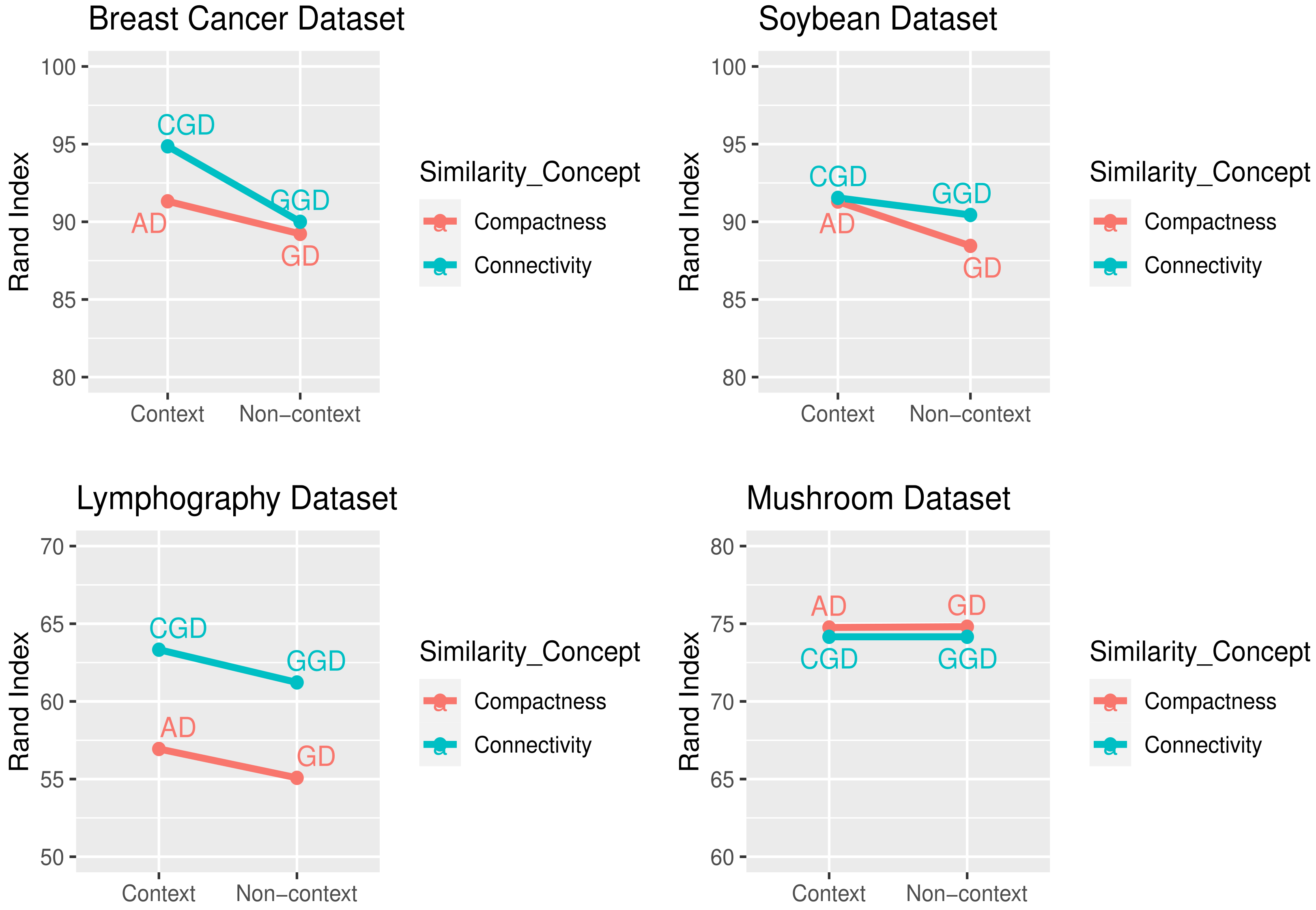
For illustrative purposes, we first present a simple example of calculating the association-based dissimilarities between two values in a categorical variable using an artificial dataset. Secondly, we demonstrate the development of the mutual k-nearest neighbor graph with various k values. Then, finally, we conducted experiments to study the characteristics of the proposed method (CGD) and compared it with other conventional categorical distance measures in the literature: Gower distance (GD) [5], association-based dissimilarity (AD) [8], and a variant of the geodesic distance using Gower distance (hereafter, Gower-based geodesic distance (GGD)).

These four different dissimilarity measures can be categorized in terms of context/non-context for consideration of correlations and compactness/connectivity for similarity concepts, as shown in

Table 1. Categorization of four dissimilarity measures.

	Compactness	Connectivity
Context	Association-based dissimilarity	Content-based geodesic dissimilarity
	(AD)	(CGD)
Non-context	Gower distance	Gower-based geodesic distance
	(GD)	(GGD)

.

4.1. Association-Based Dissimilarity (AD) between Two Values in Categorical Variable

To illustrate the calculation of the dissimilarity between two values with respect to a categorical variable, we introduce a simple artificial example as follows. Suppose that the dataset x consists of only two categorical variables “Shape” and “Color”. Shape has three categorical values: square $(\square )$, diamond $(♢)$ and triangle $(▵)$. Color has two categorical values: white (W) and black (B).

Table 2. Co-occurrence and conditional probability between Color and Shape.

	Contingent Table			Contingent Probability Table
	White (W)	Black (B)	Sum	$\mathit{p}\left(\mathit{W}\right|.)$	$\mathit{p}\left(\mathit{B}\right|.)$	Sum
□	30	40	70	$\frac{3}{7}$	$\frac{4}{7}$	1
♢	20	10	30	$\frac{2}{3}$	$\frac{1}{3}$	1
△	25	25	50	$\frac{1}{2}$	$\frac{1}{2}$	1

displays the contingent table and contingent probability table. Then, the dissimilarities of the value pairs ($\square ,♢$), ($\square ,▵$), and ($♢,▵$) can be obtained using Equations (2) and (3) as follows:

$$\begin{array}{cc}\hfill d_A(\square ,♢)& =\frac{1}{\sqrt{2}}\sqrt{{\left(\sqrt{3/7}-\sqrt{2/3}\right)}^2+{\left(\sqrt{4/7}-\sqrt{1/3}\right)}^2}=0.170\hfill \\ \hfill d_A(\square ,▵)& =\frac{1}{\sqrt{2}}\sqrt{{\left(\sqrt{3/7}-\sqrt{1/2}\right)}^2+{\left(\sqrt{4/7}-\sqrt{1/2}\right)}^2}=0.051\hfill \\ \hfill d_A(♢,▵)& =\frac{1}{\sqrt{2}}\sqrt{{\left(\sqrt{2/3}-\sqrt{1/2}\right)}^2+{\left(\sqrt{1/3}-\sqrt{1/2}\right)}^2}=0.120\hfill \end{array}$$

4.2. Mutual k-Nearest Neighbor Graph with Various k Values

The following example demonstrates the development of the mutual k-nearest neighbor graph with various k values.

Table 3. Fragments of the Mushroom dataset.

No.	Cap-Shape	Cap-Surface	Cap-Color	Bruises	Odor
1	convex	smooth	yellow	yes	almond
2	bell	smooth	white	yes	anise
3	convex	smooth	gray	no	none
4	convex	scaly	yellow	yes	almond
5	bell	smooth	white	yes	almond
6	bell	scaly	white	yes	anise
7	convex	smooth	white	no	creosote
8	convex	smooth	pink	no	creosote
9	convex	fibrous	gray	no	foul
10	convex	fibrous	gray	no	foul
11	convex	fibrous	gray	no	creosote
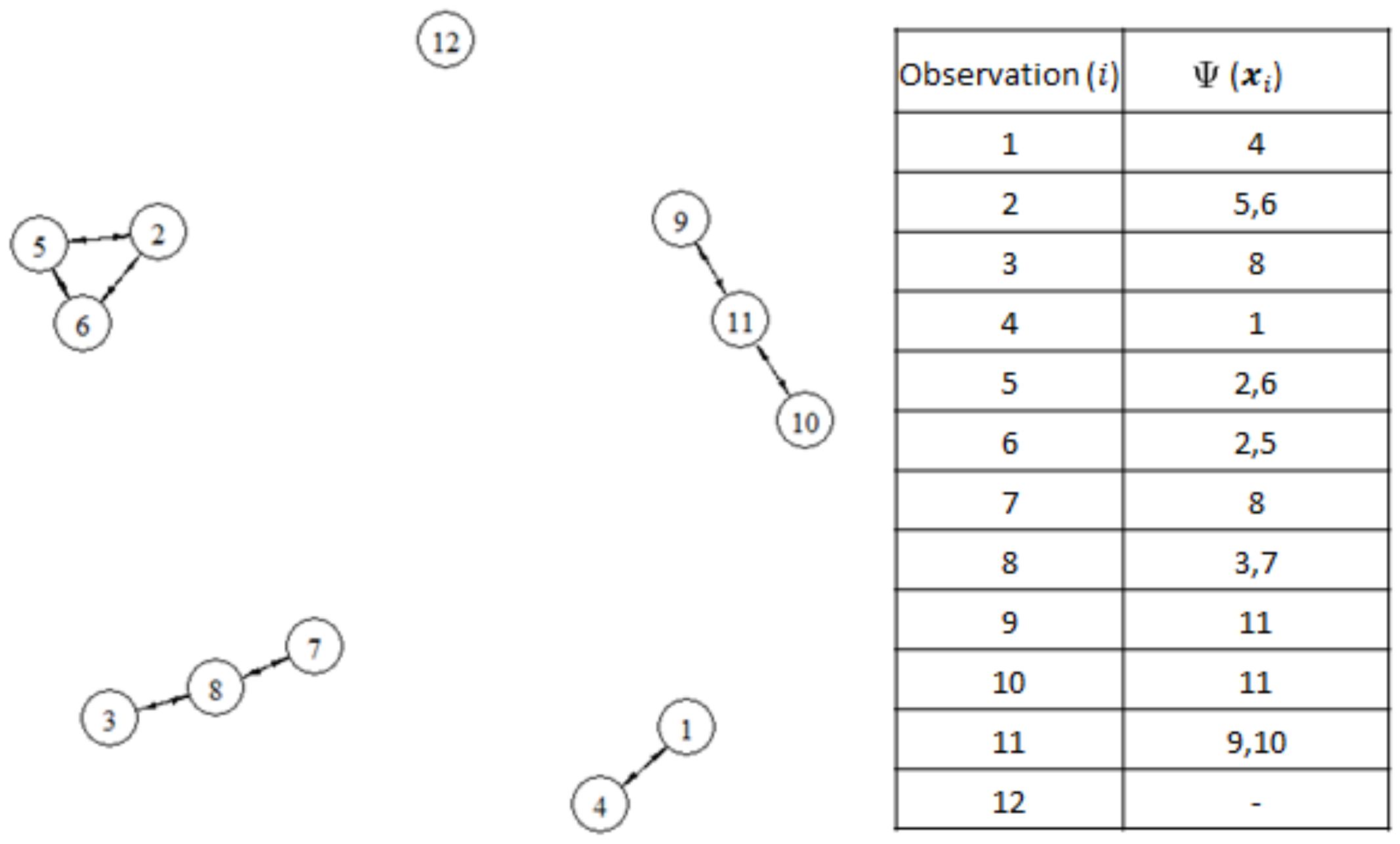
12	convex	scaly	yellow	no	foul

shows a fragment of the Mushroom dataset from UCI Machine Learning Repository (http://archive.ics.uci.edu, accessed on 5 May 2021). Let us assume that there is a dataset with 12 observations, which consist of five categorical variables; Cap-shape, Cap-surface, Cap-color, Bruises, and Odor.

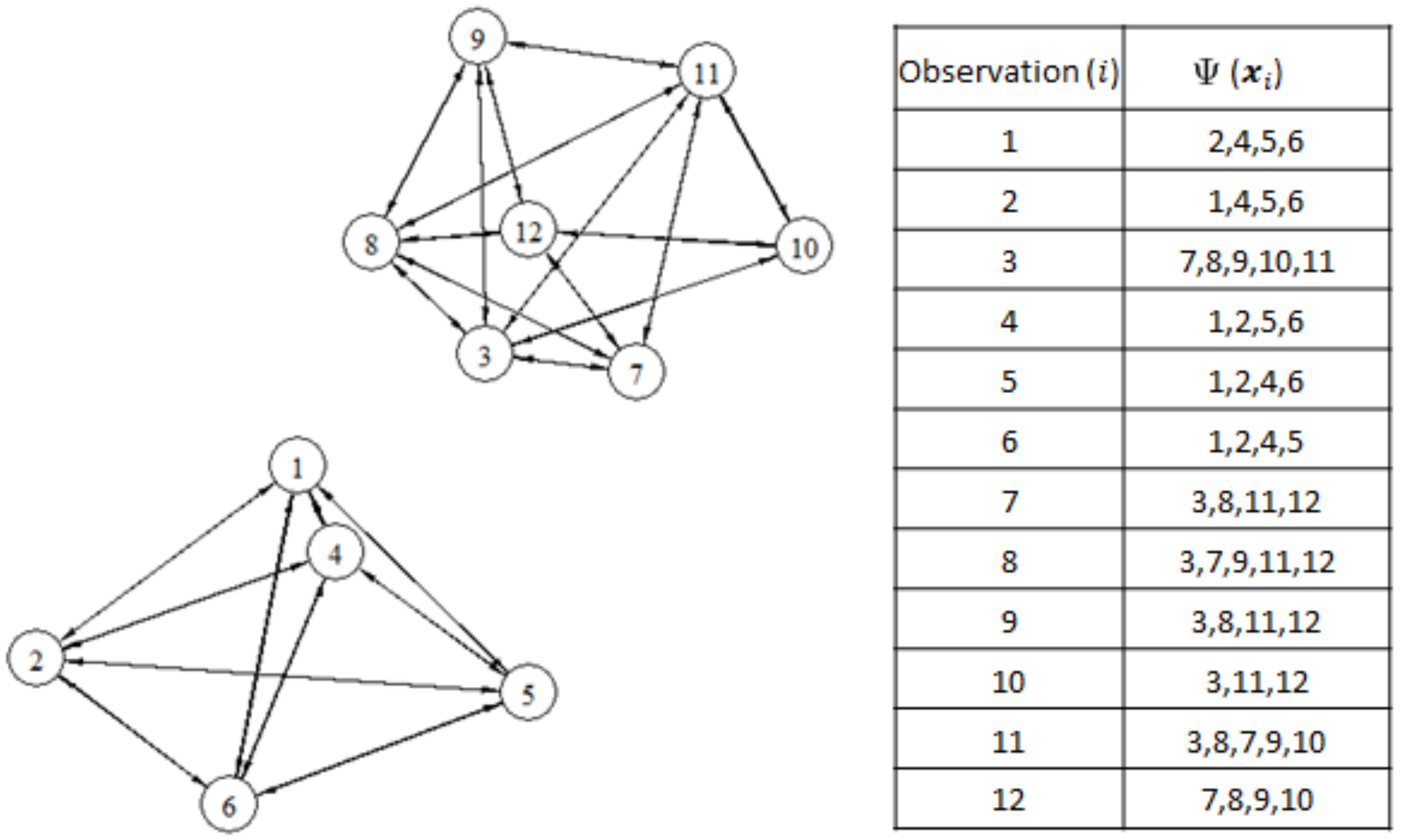
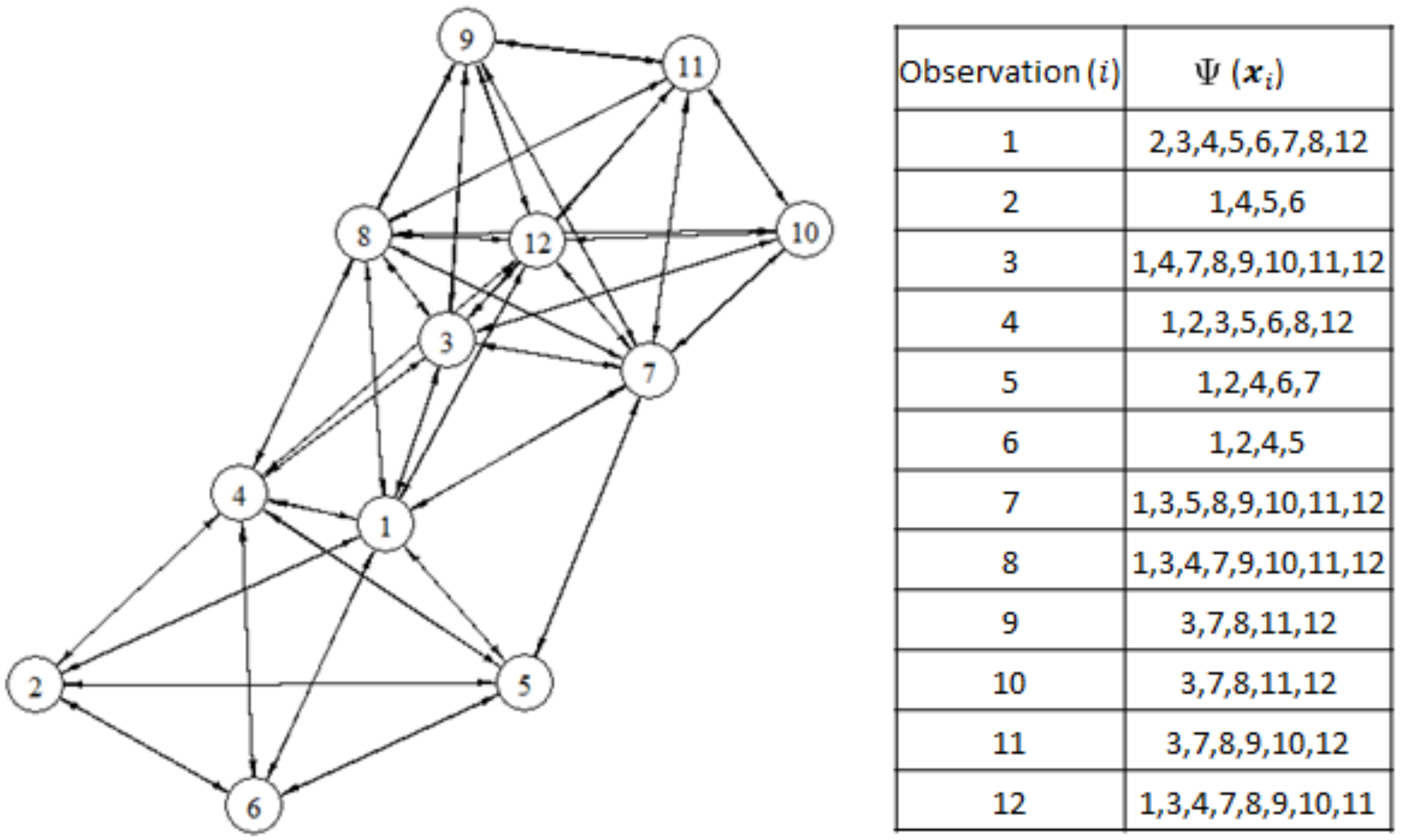
Figure 1, Figure 2 and Figure 3 illustrate the results of mutual neighborhood sets and the corresponding mutual neighborhood graphs when k is 3, 6, or 9, respectively. The neighborhood links between nodes (observations) are represented by the arrows. For example, no node belongs to the 3-mutual nearest neighbors of node ${\mathbf{x}}_{12}$ in Figure 1. The 6-mutual nearest neighbors of node ${\mathbf{x}}_{12}$ are node ${\mathbf{x}}_7$, ${\mathbf{x}}_8$, ${\mathbf{x}}_9$, and ${\mathbf{x}}_{10}$ in Figure 2. The 9-mutual nearest neighbors of node ${\mathbf{x}}_{12}$ are nodes ${\mathbf{x}}_1$, ${\mathbf{x}}_3$, ${\mathbf{x}}_4$, ${\mathbf{x}}_7$, ${\mathbf{x}}_8$, ${\mathbf{x}}_9$, ${\mathbf{x}}_{10}$, and ${\mathbf{x}}_{11}$ in Figure 3. Thus, the structure of the graph depends on the parameter k. When k increases, the size of the mutual neighborhood set of a node increases. As mentioned previously, the mutual k-nearest neighbor graph itself can produce clusters, and the number of clusters depends on the parameter k. However, if we intend to produce a larger number of clusters, the proposed context-based geodesic dissimilarity (CGD) measure between the objects in a graph is still required.

4.3. Comparative Study Using Real-Life Datasets

In our experiments, a clustering algorithm is applied to four benchmark datasets: (1) Breast cancer, (2) Soybean, (3) Lymphography, and (4) Mushroom, which were from the UCI Machine Learning Repository [35]. All datasets, except the Lymphography dataset, have missing values. In this study, we simply eliminate the observations with missing values. Furthermore, the Lymphography dataset is originally composed of eighteen variables in total, including three continuous variables and fifteen categorical (nominal) variables so that three of these continuous variables are forcibly discretized into categorical (ordinal) variables.

Table 4. Dataset information including the dependency factor.

	Breast Cancer	Soybean	Lymphography	Mushroom
Number of Nodes	683	562	148	5644
Number of Nominal variables	4	30	15	22
Number of Ordinal variables	5	5	3	0
Number of Classes	2	15	4	2
Dependency factor ($\rho \left(\mathbf{x}\right)$)	100%	61.18%	47.76%	97.62%

summarizes these datasets, including the results of the dependency analysis. Before we conducted the experiments of applying a clustering algorithm to those four benchmark datasets, we performed a dependency analysis in the same manner in [8] to find how significantly correlated several categorical variables are. For each dataset x, we evaluate the categorical data dependency using the dependency factor $\rho \left(\mathbf{x}\right)$, which is the proportion of the number of dependent categorical variable pairs in the total number of categorical variable pairs. The dependency factor is calculated by the following equation

$$\rho \left(\mathbf{x}\right)=\frac{\mathrm{Number}\mathrm{of}\mathrm{dependent}\mathrm{categorical}\mathrm{variable}\mathrm{pairs}}{p(p-1)},$$

(9)

where p is the number of variables. To test the dependency of two categorical variables, we used the chi-square statistic with a significance level of 0.05. The dependency factor has a value of 0–1, where 0 indicates that all categorical variable pairs are independent, and 1 indicates that all categorical variable pairs are dependent at the significance level of 0.05. Most of the categorical variables in the selected real-life datasets are correlated, as shown in Table 4. We believe that these real-life datasets can adequately illustrate the usefulness of the proposed method.

For clustering, we used the Partition Around Medoid (PAM) clustering algorithm [36] to study the performance of the proposed method.

The PAM algorithm is the most well-known heuristic solution for the k-medoids clustering [14,37]. The k-medoids clustering is more robust to outliers than the k-means clustering algorithms [38] and can work using a dissimilarity matrix, which is defined by any dissimilarity measure (our proposed method provides only a dissimilarity matrix, not the node (observation) coordinates). Hence, the PAM algorithm is used to compare our proposed method with the existing ones.

A brief explanation of the PAM can be provided as follows; given K initial medoids that create K clusters, each node becomes assigned to one of the K medoids that is nearest to the node. A medoid can be defined as the node of a cluster whose average dissimilarity to all nodes in the cluster is minimal. The PAM minimizes the objective function by iteratively swapping all non-medoid points and medoids until convergence [36]. The objective function of the PAM is to minimize the sum of the dissimilarities from a node to its cluster medoids.

To quantify the PAM clustering performance, the clustering validity measure is required. Based on the available knowledge about the true class membership of the dataset, the whole clustering validity measures can be divided into two sets; internal and external validity measures [39]. Internal validity measures only exploit the distribution of the dataset. On the other hand, external validity measures assume some external information, such as class membership information. It is obvious that external validity measures give less vague results than the internal validity measures as the association of the cluster points with the class membership is assumed to be known in the case of external validity measures. In our study, since the main contribution that we intend to make is to investigate the potential of using our proposed dissimilarity measure, we assume that the class information and class correspondence of the observations are already known, and the number of true clusters K is known to be equal to the number of true classes. In [39], they compared five external validity measures (namely Rand index, Jaccard index, Folkes–Mallows index, Rogers–Tanimoto index and Kulczynski index) to observe the performance of different clustering validity measures as the number of attributes increased for the same algorithm when others such as the number of instances and the number of classes were almost invariant. As a conclusion, the external validity measures were all consistent [39]. The authors reported that all of the external validity measures produced different values but the same ranks. In the same manner as in [39], we applied all five external validity measures (Rand index, Jaccard index, Folkes–Mallows index, Rogers–Tanimoto index and Kulczynski index) for our comparison study, as shown in Table 6. The results were consistent with [39], that is, the ranks of each dissimilarity measure were identical no matter which external validity measure is used. Therefore, here we explain only the Rand index among the external validity measures, which is the most popular external validity measure.

The Rand index (RI) [40] has been widely used to calculate the clustering performance [41,42,43]. The RI is basically a measure of the similarity between two clusterings results. Let us assume that two clustering results share a cluster membership; then the similarity between two clustering results is calculated as follows

$$RI=\frac{a+b}{\left(\genfrac{}{}{0pt}{}{n}{2}\right)},$$

(10)

where a is the number of pairs of nodes with the common cluster memberships, b is the number of pairs of nodes with nonidentical cluster memberships, and n is the number of nodes. The RI has a value of 0–1, where 0 implies that the two results do not agree on any pair of clustering memberships, and 1 indicates that the two clustering memberships are exactly identical. If the dataset has a true cluster membership, this true cluster membership becomes a reference membership. Therefore, the RI evaluates the agreement between the true cluster membership and the PAM clustering results [44]. A large RI indicates that the true cluster membership can be correctly recovered by the PAM clustering results.

To apply the PAM with a geodesic distance framework such as the GGD and the proposed CGD, two parameters must be predetermined, such as the parameter k for the mutual k-nearest neighbor graph construction and K for the number of clusters. As mentioned earlier, we assumed that the number of true clusters K is known to be equal to the number of true classes. However, there is no concrete guideline for selecting the optimal parameters k. Hence, we attempted to heuristically decide only the parameter k, in a similar manner used in Yu and Kim [14]. They varied the values of k from 3 to 30 and determined the parameter k that yielded the best performance. Thus, we focus on only determining a proper k that yields the largest RI while varying the values of k. In our study, the RI was calculated by changing k from 3 to 60. The smallest k obtained from the largest RI is summarized in

Table 5. Smallest k with the largest Rand index.

Data Set	Gower-Based	Proposed Method
	Geodesic Distance	(Context-Based Geodesic Dissimilarity)
Breast cancer	9	52
Soybean	36	40
Lymphography	14	39
Mushroom	13	21

.

Table 6. Comparison of the clustering performance on four real-life datasets.

Data Set	Rand Index
	Gower	Association-Based	Gower-Based	Proposed
	Distance	Dissimilarity	Geodesic Distance	Method
	(GD)	(AD)	(GGD)	(CGD)
Breast cancer	89.22%	91.32%	90.00%	94.86%
Soybean	89.45%	91.30%	90.44%	91.54%
Lymphography	55.08%	56.94%	61.11%	63.33%
Mushroom	74.81%	74.76%	74.16%	74.16%
Data Set	Jaccard Index
	Gower	Association-Based	Gower-Based	Proposed
	Distance	Dissimilarity	Geodesic Distance	Method
	(GD)	(AD)	(GGD)	(CGD)
Breast cancer	82.34%	85.36%	83.08%	90.97%
Soybean	21.98%	34.81%	27.14%	35.22%
Lymphography	24.60%	26.25%	29.80%	33.01%
Mushroom	64.37%	64.34%	63.92%	63.92%
Data Set	Folkes–Mallows Index
	Gower	Association-Based	Gower-Based	Proposed
	Distance	Dissimilarity	Geodesic Distance	Method
	(GD)	(AD)	(GGD)	(CGD)
Breast cancer	90.34%	92.11%	90.76%	95.27%
Soybean	37.16%	52.16%	43.87%	52.79%
Lymphography	40.86%	43.14%	48.11%	51.74%
Mushroom	78.66%	78.64%	78.39%	78.39%
Data Set	Rogers–Tanimoto Index
	Gower	Association-Based	Gower-Based	Proposed
	Distance	Dissimilarity	Geodesic Distance	Method
	(GD)	(AD)	(GGD)	(CGD)
Breast cancer	80.53%	84.03%	81.82%	90.22%
Soybean	80.91%	84.00%	82.55%	84.40%
Lymphography	38.01%	39.80%	44.00%	46.34%
Mushroom	59.76%	59.69%	58.94%	58.94%
Data Set	Kulczynski Index
	Gower	Association-Based	Gower-Based	Proposed
	Distance	Dissimilarity	Geodesic Distance	Method
	(GD)	(AD)	(GGD)	(CGD)
Breast cancer	90.36%	92.11%	90.76%	95.27%
Soybean	38.31%	52.69%	45.07%	53.49%
Lymphography	42.29%	44.76%	50.40%	53.93%
Mushroom	78.99%	78.98%	78.79%	78.79%

shows the comparative results of the PAM algorithms in terms of five different external validity measures using various distance/dissimilarity measures (GD, AD, GGD, and CGD). The results shown in Table 6 will be discussed in the following section.

5. Discussion

The results shown in Table 6 indicate that the proposed method shows better performance compared to the other measures, since it produces larger RI values than other measures for three of four datasets (Breast cancer, Soybean, and Lymphography), with the exception of the Mushroom dataset. That is, for Breast cancer, Soybean, and Lymphography datasets, the proposed method yields the highest scores 94.86%, 91.32%, and 63.33%, respectively. For the Mushroom dataset, various distance measures yield almost identical Rand indices with less than 1% point differences (GD 74.81%, AD 74.76%, GGD 74.16%, and the proposed method CGD 74.16%). This result demonstrates that the proposed measure generally facilitates the discovery of the natural groupings well compared to the other dissimilarity measures.

Figure 4 presents a visual comparison using the result of the Rand index in Table 1 and categorization in Table 6. Except for the Mushroom dataset, in general, the dissimilarity measures with context-based method considering the correlation between categorical variables (such as AD and CGD) show better performances than others (such as GD and GGD). This result may indicate that since these three datasets (Breast cancer, Soybean, Lymphography) have highly correlated categorical variables (as shown in Table 4, that is, dependency factor ($\rho \left(\mathbf{x}\right)$) for Breast cancer 100%, Soybean 61.18%, and Lymphography 47.76%), the context-based methods outperform the non-context-based methods. In addition, the dissimilarity measures that consider the concept of connectivity of data observations (such as GGD and CGD) perform better than those that do not (such as GD and AD). This result may also indicate that these three datasets have clusters of complex shapes in their manifold structure.

In the case of the Mushroom dataset with a high value of dependency factor (97% as shown in Table 4), all four dissimilarity measures showed similar performances with slight differences. That is, the concept of context did not improve the performance of clustering. We might interpret it in a way that this dataset has many correlated variables but no high correlation between variables. The reason why the concept of connectivity was not effective in the performance of clustering for this dataset may also be interpreted in a way in which the dataset has significant noise and does not reveal complex shapes in a manifold structure.

Overall, the proposed context-based geodesic dissimilarity (CGD) measure that considers the correlations among categorical variables and the concept of connectivity has, in general, better clustering quality when categorical variables are highly correlated and the dataset has clusters of complex shapes.

6. Conclusions

In this study, we have proposed a novel dissimilarity measure for the categorical data clustering problem. The proposed method can effectively accommodate the nonlinear and complex patterns of the categorical dataset. It discovers the implicit topological structures in the categorical data and considers the relationships among the categorical variables. Our experimental results reveal that the categorical data can also have implicit data patterns and confirm that the dissimilarity measure that considers both data patterns and relationships among the categorical variables generally yields better clustering performance than other dissimilarity measures.

Despite its successful performance in categorical data clustering, there are some open issues with the current research. For example, the issue of computation burden of our proposed method is not theoretically investigated. If the data consist of many categorical variables, variable selection may be necessary to avoid the curse of dimensionality. Meanwhile, a context-based approach such as the proposed method cannot guarantee successful performance for the data that are composed of completely independent categorical variables. Although these research ideas are beyond the scope of this paper, they will be an interesting direction for future research.