
Birds Eye View Look-Up Table Estimation with Semantic Segmentation


Abstract
:1. Introduction
2. Related Work
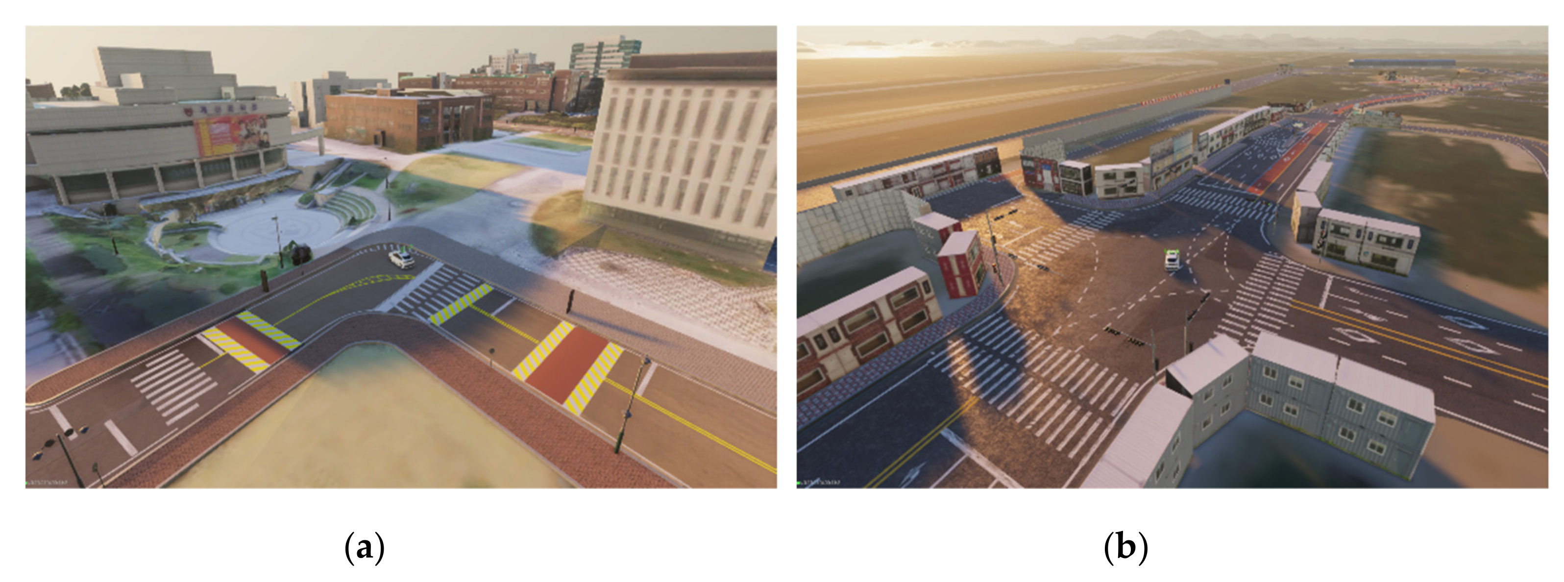
3. Synthetic Database
3.1. Data Collection
3.2. LUT Generation
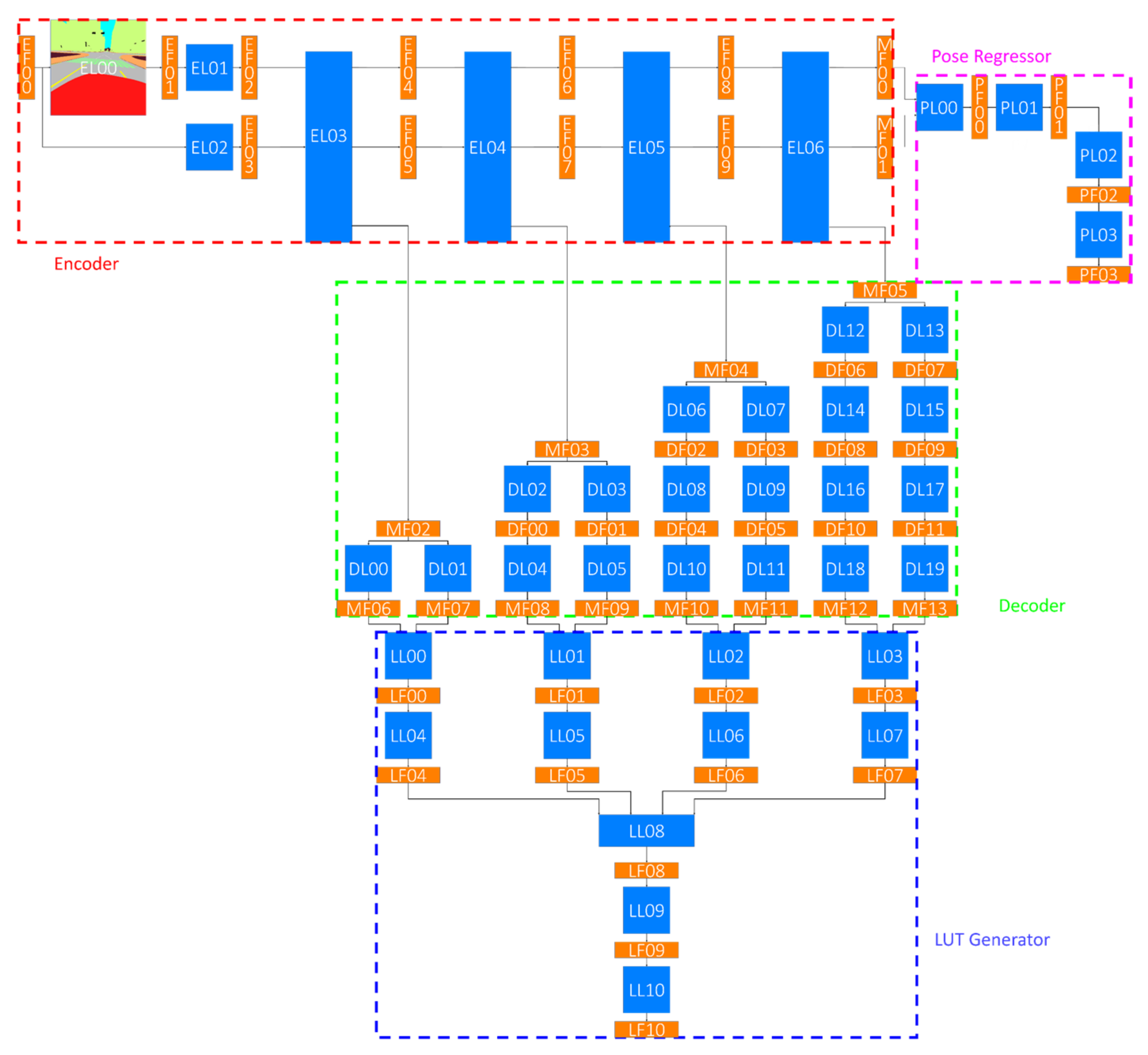
4. Proposed Deep Learning Network
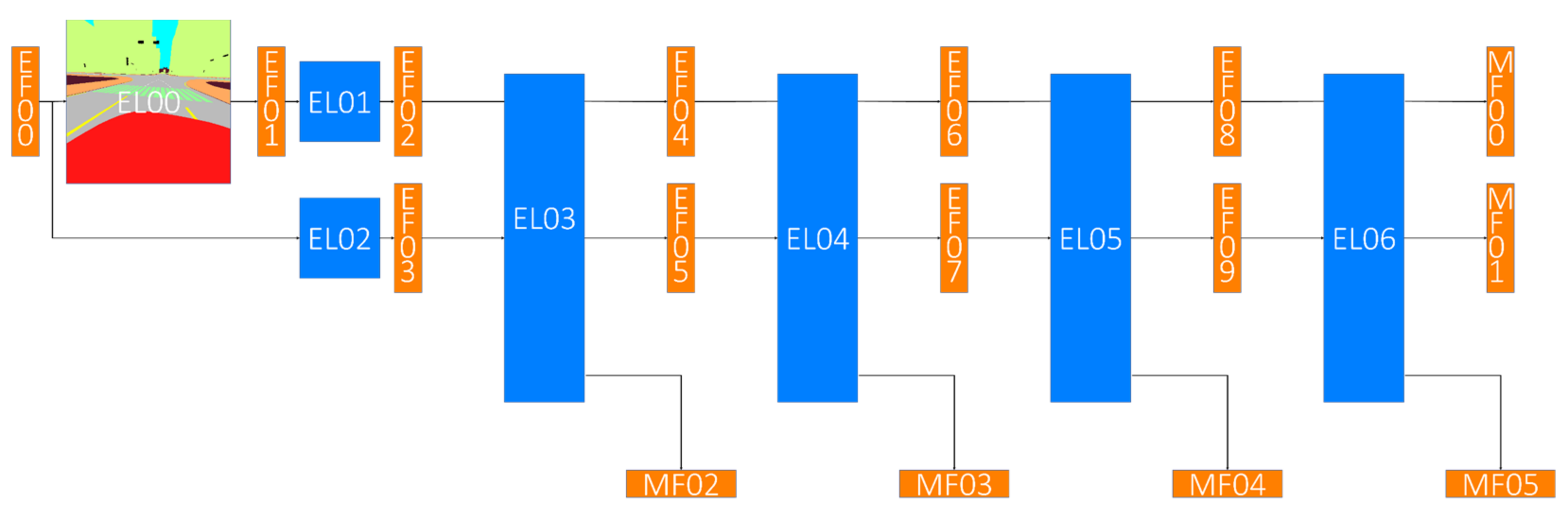
4.1. Encoder
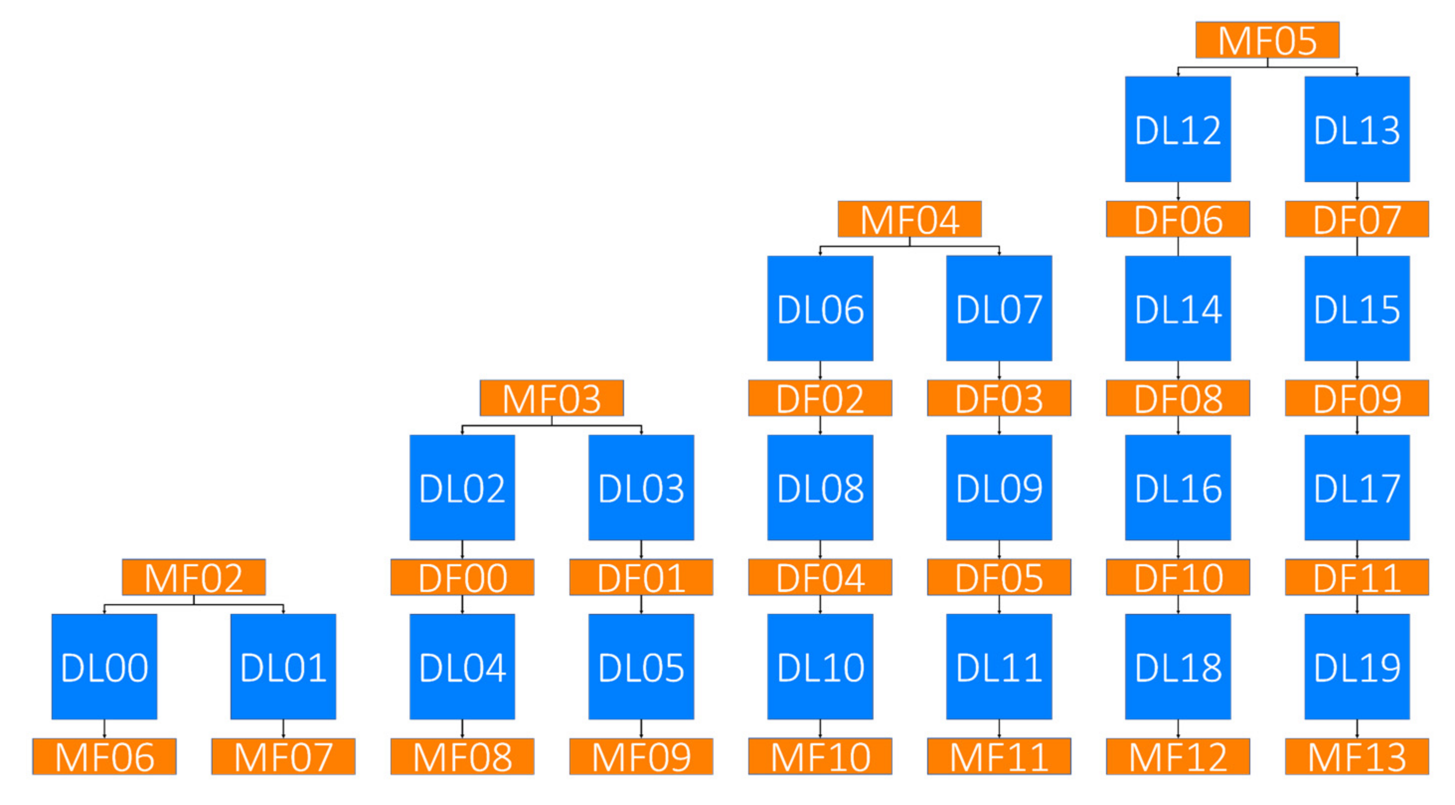
4.2. Decoder
4.3. LUT Generator
4.4. Pose Regressor
5. Experiments
5.1. Loss Cost
5.2. Quantitative Evaluation
5.3. Qualitative Evaluation
6. Conclusions
Author Contributions
Funding
Institutional Review Board Statement
Informed Consent Statement
Data Availability Statement
Conflicts of Interest
References
- Choi, D.Y.; Choi, J.H.; Choi, J.W.; Song, B.C. CNN-based Pre-Processing and Multi-Frame-Based View Transformation for Fisheye Camera-Based AVM System. In Proceedings of the 2017 IEEE International Conference on Image Processing (ICIP), Beijing, China, 17–20 September 2017. [Google Scholar]
- Zhu, X.; Yin, Z.; Shi, J.; Li, H.; Lin, D. Generative Adversarial Frontal View to Bird View Synthesis. In Proceedings of the 2018 International conference on 3D Vision (3DV), Verona, Italy, 5–8 September 2018. [Google Scholar]
- Chao, P.; Kao, C.Y.; Ruan, Y.S.; Huang, C.H.; Lin, Y.L. HarDNet: A low memory traffic network. In Proceedings of the IEEE/CVF International Conference on Computer Vision (ICCV), Seoul, Korea, 27 October–2 November 2019. [Google Scholar]
- Hong, Y.; Pan, H.; Sun, W.; Jia, Y. Deep Dual-resolution Networks for Real-time and Accurate Semantic Segmentation of Road Scenes. arXiv 2021, arXiv:2101.06085. [Google Scholar]
- Tao, A.; Sapra, K.; Catanzaro, B. Hierarchical Multi-scale Attention for Semantic Segmentation. arXiv 2020, arXiv:2005.10821. [Google Scholar]
- Mehta, S.; Rastegari, M.; Caspi, A.; Shapiro, L.; Hajishirzi, H. ESPNet: Efficient Spatial Pyramid of Dilated Convolutions for Semantic Segmentation. In Proceedings of the European Conference on Computer Vision (ECCV), Munich, Germany, 8–14 September 2018. [Google Scholar]
- Hsu, C.M.; Chen, J.Y. Around View Monitoring-Based Vacant Parking Space Detection and Analysis. Appl. Sci. 2019, 9, 3403. [Google Scholar] [CrossRef] [Green Version]
- Lee, D.; Lee, J.S.; Lee, S.; Kee, S.C. The Real-time Implementation for the Parking Line Departure Warning System. In Proceedings of the 3rd IEEE International Conference on Intelligent Transportation Engineering (ICITE), Singapore, 3–5 September 2018. [Google Scholar]
- Dhall, A.; Chelani, K.; Radhakrishnan, V.; Krishna, K.M. LiDAR-Camera Calibration using 3D-3D Point correspondences. arXiv 2017, arXiv:1705.09785. [Google Scholar]
- Lee, D.; Kee, S.C. Real-time Implementation of the Parking Line Departure Warning System Using Partitioned Vehicle Region Images. Trans. KSAE 2019, 7, 553–560. [Google Scholar]
- Le, H.; Liu, F.; Zhang, S.; Agarwala, A. Deep Homography Estimation for Dynamic Scenes. In Proceedings of the IEEE/CVF Conference on Computer Vision and Pattern Recognition (CVPR), Seattle, WA, USA, 13–19 June 2020. [Google Scholar]
- Jaderberg, M.; Simonyan, K.; Zisserman, A. Spatial Transformer Networks. In Proceedings of the Conference on Neural Information Processing Systems (NIPS), Montreal, QC, Canada, 7–12 December 2015. [Google Scholar]
- Ronneberger, O.; Fischer, P.; Brox, T. U-net: Convolutional Networks for Biomedical Image Segmentation. In Proceedings of the International Conference on Medical Image Computing and Computer-Assisted Intervention (MICCAI), Munich, Germany, 5–9 October 2015. [Google Scholar]
- Lin, T.Y.; Maire, M.; Belongie, S.; Hays, J.; Perona, P.; Ramanan, D.; Zitnick, C.L. Microsoft COCO: Common Objects in Context. In Proceedings of the European Conference on Computer Vision (ECCV), Zurich, Switzerland, 6–12 September 2014. [Google Scholar]
- Geiger, A.; Lenz, P.; Stiller, C.; Urtasun, R. Vision meets Robotics: The KITTI Dataset. Int. J. Robot. Res. 2013, 32, 1231–1237. [Google Scholar] [CrossRef] [Green Version]
- MORAI Sim Standard. Available online: http://www.morai.ai (accessed on 30 August 2021).
- He, K.; Zhang, X.; Ren, S.; Sun, J. Deep Residual Learning for Image Recognition. In Proceedings of the IEEE Conference on Computer Vision and Pattern Recognition (CVPR), Las Vegas, NV, USA, 27–30 June 2016. [Google Scholar]
- Shi, W.; Caballero, J.; Huszár, F.; Totz, J.; Aitken, A.P.; Bishop, R.; Wang, Z. Real-time single image and video super-resolution using an efficient sub-pixel convolutional neural network. In Proceedings of the IEEE Conference on Computer Vision and Pattern Recognition, Las Vegas, NV, USA, 27–30 June 2016. [Google Scholar]
- LeCun, Y.; Boser, B.; Denker, J.S.; Henderson, D.; Howard, R.E.; Hubbard, W.; Jackel, L.D. Backpropagation applied to handwritten zip code recognition. Neural Comput. 1989, 1, 541–551. [Google Scholar] [CrossRef]
- Rubenstein, R.Y.; Kroese, D.P.; Cohen, I.; Porotsky, S.; Taimre, T. Cross-Entropy Method; Springer: Boston, MA, USA, 2013. [Google Scholar]


| (a) | ||||
| Name | In Channels | Out Channels | Layer | Remarks |
| EL00 | 3 | C | Semantic segmentation | Encoder layer |
| EL01 | C | 16 | 2D convolution (kernel: 3; stride: 1; padding: 1) | |
| EL02 | 3 | 16 | ||
| EL03 | 16 | 64 | Compress block | |
| EL04 | 64 | 256 | ||
| EL05 | 256 | 1024 | ||
| EL06 | 1024 | 4096 | ||
| (b) | ||||
| Name | Channel | Height | Width | Remarks |
| EF00 | 3 | H | W | Encoder feature |
| EF01 | C | H | W | |
| EF02 | 16 | H | W | |
| EF03 | ||||
| EF04 | 64 | H/2 | W/2 | |
| EF05 | ||||
| EF06 | 256 | H/4 | W/4 | |
| EF07 | ||||
| EF08 | 1024 | H/8 | W/8 | |
| EF09 | ||||
| MF00 | 4096 | H/16 | W/16 | Middle feature |
| MF01 | ||||
| MF02 | 64 | H/2 | W/2 | |
| MF03 | 256 | H/4 | W/4 | |
| MF04 | 1024 | H/8 | W/8 | |
| MF05 | 4096 | H/16 | W/16 | |
| (a) | ||||
| Name | In Channels | Out Channels | Layer | Remarks |
| CL00 | C | 4C | Custom residual block | Compress layer |
| CL01 | ||||
| CL02 | 4C | 8C | Concatenate | |
| CL03 | 8C | 4C | 2D convolution (kernel: 3; stride: 1; padding: 1) | |
| (b) | ||||
| Name | Channel | Height | Width | Remarks |
| CF00 | C | H | W | Compress feature |
| CF01 | ||||
| CF02 | 4C | H/2 | W/2 | |
| CF03 | ||||
| CF04 | 8C | H/2 | W/2 | |
| CF05 | 4C | H/2 | W/2 | |
| CF06 | ||||
| CF07 | ||||
| (c) | ||||
| Name | In Channels | Out Channels | Layer | Remarks |
| RL00 | C | 2C | 2D convolution (kernel: 3; stride: 2; padding: 1) | Residual layer |
| RL01 | 2C | 4C | 2D convolution (kernel: 3; stride: 1; padding: 1) | |
| RL02 | C | 4C | 2D convolution (kernel: 3; stride: 2; padding: 1) | |
| RL03 | 4C | 4C | Element Add | |
| (d) | ||||
| Name | Channel | Height | Width | Remarks |
| RF00 | C | H | W | Residual feature |
| RF01 | 2C | H/2 | W/2 | |
| RF02 | 4C | H/2 | W/2 | |
| RF03 | 4C | H/2 | W/2 | |
| RF04 | 4C | H/2 | W/2 | |
| (a) | ||||
| Name | In Channels | Out Channels | Layer | Remarks |
| DL00 | 64 | 16 | Pixel shuffle | Decoder layer |
| DL01 | 64 | 16 | Convolution transposed (kernel: 2; stride: 2; padding: 0) | |
| DL02 | 256 | 64 | Pixel shuffle | |
| DL03 | 256 | 64 | Convolution transposed (kernel: 2; stride: 2; padding: 0) | |
| DL04 | 64 | 16 | Pixel shuffle | |
| DL05 | 64 | 16 | Convolution transposed (kernel: 2; stride: 2; padding: 0) | |
| DL06 | 1024 | 256 | Pixel shuffle | |
| DL07 | 1024 | 256 | Convolution transposed (kernel: 2; stride: 2; padding: 0) | |
| DL08 | 256 | 64 | Pixel shuffle | |
| DL09 | 256 | 64 | Convolution transposed (kernel: 2; stride: 2; padding: 0) | |
| DL10 | 64 | 16 | Pixel shuffle | |
| DL11 | 64 | 16 | Convolution transposed (kernel: 2; stride: 2; padding: 0) | |
| DL12 | 4096 | 1024 | Pixel shuffle | |
| DL13 | 4096 | 1024 | Convolution transposed (kernel: 2; stride: 2; padding: 0) | |
| DL14 | 1024 | 256 | Pixel shuffle | |
| DL15 | 1024 | 256 | Convolution transposed (kernel: 2; stride: 2; padding: 0) | |
| DL16 | 256 | 64 | Pixel shuffle | |
| DL17 | 256 | 64 | Convolution transposed (kernel: 2; stride: 2; padding: 0) | |
| DL18 | 64 | 16 | Pixel shuffle | |
| DL19 | 64 | 16 | Convolution transposed (kernel: 2; stride: 2; padding: 0) | |
| (b) | ||||
| Name | Channel | Height | Width | Remarks |
| DF00 | 64 | H/2 | W/2 | Decoder feature |
| DF01 | ||||
| DF02 | 256 | H/4 | W/4 | |
| DF03 | ||||
| DF04 | 64 | H/2 | W/2 | |
| DF05 | ||||
| DF06 | 1024 | H/8 | W/8 | |
| DF07 | ||||
| DF08 | 256 | H/4 | W/4 | |
| DF09 | ||||
| DF10 | 64 | H/2 | W/2 | |
| DF11 | ||||
| MF02 | 64 | H/2 | W/2 | Middle feature |
| MF03 | 256 | H/4 | W/4 | |
| MF04 | 1024 | H/8 | W/8 | |
| MF05 | 4096 | H/16 | W/16 | |
| MF06 | 16 | H | W | |
| MF07 | ||||
| MF08 | ||||
| MF09 | ||||
| MF10 | ||||
| MF11 | ||||
| MF12 | ||||
| MF13 | ||||
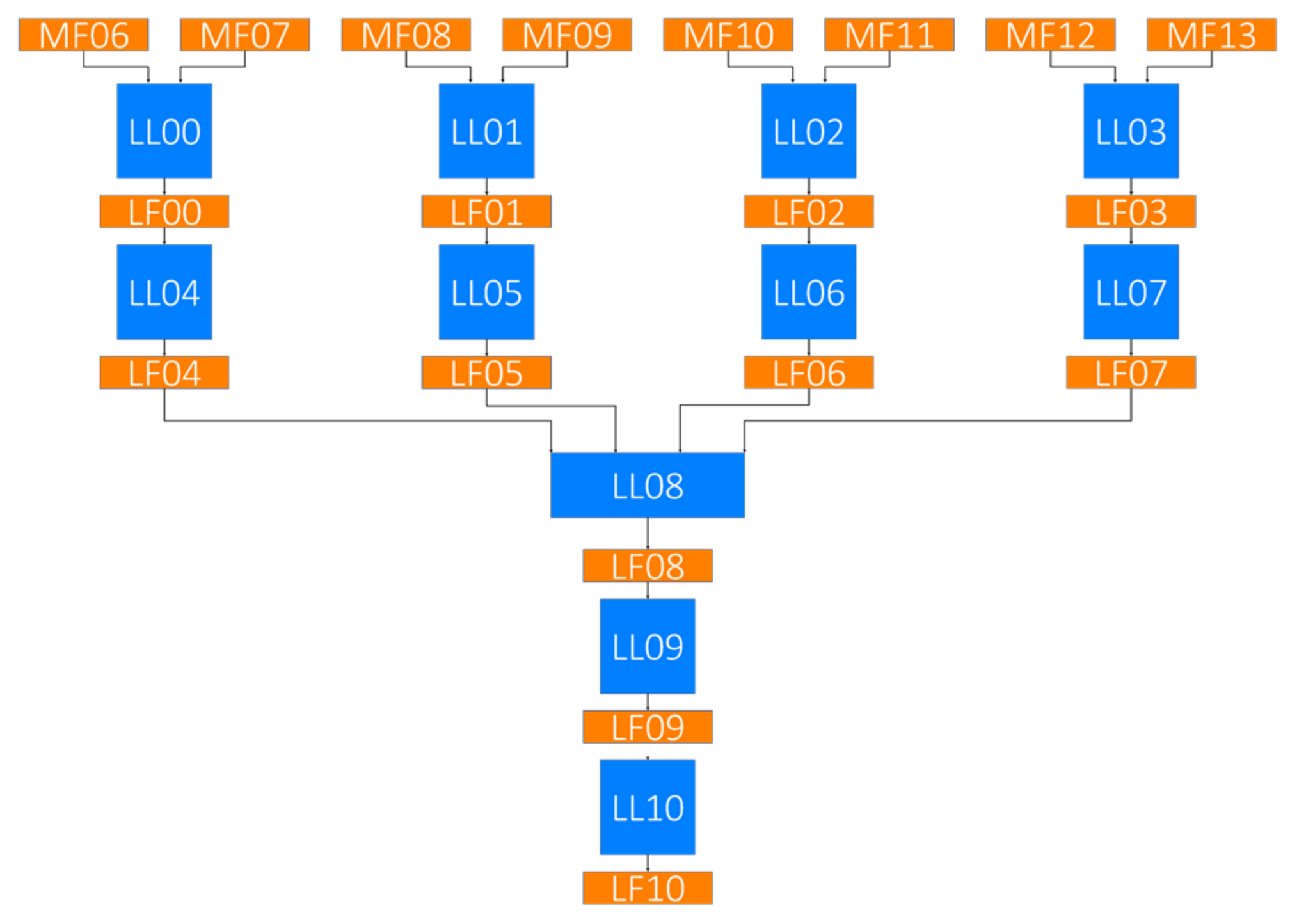
| (a) | ||||
| Name | In Channels | Out Channels | Layer | Remarks |
| LL00 | 16 | 32 | Concatenate | LUT layer |
| LL01 | ||||
| LL02 | ||||
| LL03 | ||||
| LL04 | 32 | 16 | 2D convolution (kernel: 3; stride: 1; padding: 1) | |
| LL05 | ||||
| LL06 | ||||
| LL07 | ||||
| LL08 | 16 | 64 | Concatenate | |
| LL09 | 64 | 16 | 2D convolution (kernel: 3; stride: 1; padding: 1) | |
| LL10 | 16 | 3 | 2D convolution (kernel: 3; stride: 1; padding: 1) | |
| (b) | ||||
| Name | Channel | Height | Width | Remarks |
| LF00 | 32 | H | W | LUT feature |
| LF01 | ||||
| LF02 | ||||
| LF03 | ||||
| LF04 | 16 | H | W | |
| LF05 | ||||
| LF06 | ||||
| LF07 | ||||
| LF08 | 64 | H | W | |
| LF09 | 16 | H | W | |
| LF10 | 3 | H | W | |
| MF06 | 16 | H | W | Middle feature |
| MF07 | ||||
| MF08 | ||||
| MF09 | ||||
| MF10 | ||||
| MF11 | ||||
| MF12 | ||||
| MF13 | ||||
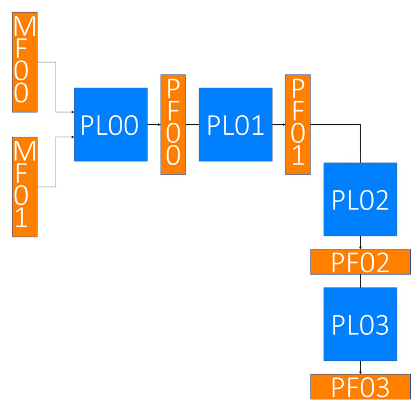
| (a) | ||||
| Name | In Channels | Out Channels | Layer | Remarks |
| PL00 | 4096 | 8192 | Concatenate | Pose layer |
| PL01 | 8192 | 1024 | 2D convolution (Kernel: 3; stride: 1; padding: 1) | |
| PL02 | 1024 | 4HW | Flatten (3D to 1D) | |
| PL03 | 4HW | 3 | Fully connected layer | |
| (b) | ||||
| Name | Channel | Height | Width | Remarks |
| PF00 | 8192 | H/16 | W/16 | Pose Feature |
| PF01 | 1024 | H/16 | W/16 | |
| PF02 | 4HW | 1 | 1 | |
| PF03 | 3 | 1 | 1 | |
| MF00 | 4096 | H/16 | W/16 | |
| MF01 | ||||
| No | Scale | Parallel Path | Pose Regressor | Processing Time (s) | Seg Loss | LUT Loss | Pose Loss |
|---|---|---|---|---|---|---|---|
| v1 | Single | 2 pixel shuffles | X | 0.18 | 0.65 | 1.59 | - |
| v2 | Single | Pixel shuffle and convolution transposed | X | 0.20 | 0.58 | 0.09 | - |
| v3 | Multi | Pixel shuffle and convolution transposed | X | 0.74 | 0.22 | 0.04 | - |
| v4 | Multi | Pixel shuffle and convolution transposed | O | 0.81 | 0.14 | 0.01 | 0.14 |
| From | To | Processing Time Change (To/From) | Seg Loss Change (To/From) | LUT Loss Change (To/From) |
|---|---|---|---|---|
| v1 | v2 | 1.11 | 0.89 | 0.06 |
| v2 | v3 | 3.70 | 0.38 | 0.44 |
| v3 | v4 | 1.09 | 0.64 | 0.25 |
| Origin |  |  |  |
| GT |  |  |  |
| v1 |  |  |  |
| v2 |  |  |  |
| v3 |  |  |  |
| v4 |  |  |  |
| Origin |  |  |  |
| GT |  |  |  |
| v1 |  |  |  |
| v2 |  |  |  |
| v3 |  |  |  |
| v4 |  |  |  |
Publisher’s Note: MDPI stays neutral with regard to jurisdictional claims in published maps and institutional affiliations. |
© 2021 by the authors. Licensee MDPI, Basel, Switzerland. This article is an open access article distributed under the terms and conditions of the Creative Commons Attribution (CC BY) license (https://creativecommons.org/licenses/by/4.0/).
Share and Cite
Lee, D.; Tay, W.P.; Kee, S.-C. Birds Eye View Look-Up Table Estimation with Semantic Segmentation. Appl. Sci. 2021, 11, 8047. https://doi.org/10.3390/app11178047
Lee D, Tay WP, Kee S-C. Birds Eye View Look-Up Table Estimation with Semantic Segmentation. Applied Sciences. 2021; 11(17):8047. https://doi.org/10.3390/app11178047
Chicago/Turabian StyleLee, Dongkyu, Wee Peng Tay, and Seok-Cheol Kee. 2021. "Birds Eye View Look-Up Table Estimation with Semantic Segmentation" Applied Sciences 11, no. 17: 8047. https://doi.org/10.3390/app11178047