Robust Flow Field Signal Estimation Method for Flow Sensing by Underwater Robotics

Abstract

The flow field is difficult to evaluate, and underwater robotics can only partly adapt to the submarine environment. However, fish can sense the complex underwater environment by their lateral line system. In order to reveal the fish flow sensing mechanism, a robust nonlinear signal estimation method based on the Volterra series model with the Kautz kernel function is provided, which is named KKF-VSM. The flow field signal around a square target is used as the original signal. The sinusoidal noise and the signal around a triangular obstacle are considered undesired signals, and the predicting performance of KKF-VSM is analyzed after introducing them locally in the original signals. Compared to the radial basis function neural network model (RBF-NNM), the advantages of KKF-VSM are not only its robustness but also its higher sensitivity to weak signals and its predicting accuracy. It is confirmed that even for strong nonlinear signals, such as pressure responses in the flow field, KKF-VSM is more efficient than the commonly used RBF-NNM. It can provide a reference for the application of the artificial lateral line system on underwater robotics, improving its adaptability in complex environments based on flow field information.

1. Introduction

The autonomous underwater vehicle (AUV) is an important tool for marine environment exploration that is widely used. Since the underwater environment is complex, the adaptability of AUV needs to be improved [1,2]. The main aim of the current study on AUV environmental adaptability is to improve its control [3,4,5,6,7]. In practical applications, it has been found that the poor environmental adaptability of AUV is due to its inability to sense the surrounding environment [8,9,10]. At present, AUVs sense the surrounding environment on the basis of a visual and an acoustic system. However, the sensing range of the underwater visual system is limited because visual signals decay rapidly in the water and are easily affected by the water quality. In the context of underwater target detection, the acoustic signal also has many issues, such as high cost and high-power consumption. In complex environments, the acoustic signal is affected and cannot be properly applied [11,12,13]. In addition, the visual and acoustic signals detect targets through reflection and are, thus, indirect signals. They are unable to capture information regarding the flow field, such as the eddy and ocean currents.

In a study of marine organisms, bionics researchers found that fish have a sensing organ that they called the lateral line system (LLS). The LLS can help fish acquire extraordinary environmental adaptability [14,15,16,17]. The LLS contains two kinds of sensory neuromasts: the superficial neuromast and the canal neuromast. The superficial neuromast can sense the magnitude and direction of flow velocity, and the canal neuromast is usually used to sense the acceleration of the flow field, such as fluctuations [18,19,20,21,22]. Fish can make adjustments to the surrounding environment based on the information from the LLS. This method can sense the physical field directly, and the sensing signal is a direct signal. This method has the advantage of being more accurate and comprehensive. However, in the natural environment, the flow field is made complex by numerous uncertain factors, which hinder the success of engineering applications [23,24,25].

Machine learning methods can be used to overcome the problem of underwater target recognition based on flow field signals. Three kinds of statistical methods are used for targets recognition, which are as follows:

• Novelty recognition: one normal, known state signal is set first. Then, the test signal is compared with the normal signal. Their difference can be used to evaluate an environmental change. In this method, a statistical threshold value is set and used to eliminate the interference [26];
• Classification recognition: All states of the system are obtained first, and then they are divided into several known types. The test signal characteristics are identified and are used to evaluate an environment change [27];
• Regression algorithms: The confidence limits of the variables are set to monitor some dynamic processes. The mathematical model of the system evolution can be obtained by a linear or nonlinear algorithm [28,29,30].

Novelty recognition and classification recognition are suitable for a steady system, and the states are known. Therefore, in the flow field system, the method based on regression algorithms is the main one and is used to build a mathematical model. Various methods can be used with regression algorithms, such as nonlinear principal component analysis [31], extreme value statistics [32], peaks over threshold [33], machine learning algorithms [34], neural networks [35], Bayesian approaches [36], Mahalanobis distance [37], and others. In all these applications, the nonlinear features of flow field changes can be obtained. However, in the natural environment, there are often multiple influencing factors superimposed on each other, causing the system to be highly nonlinear. Then some cracks, delamination, or chaotic phenomena appear [38].

In nonlinear systems, time and frequency domains are commonly used to describe nonlinear behaviors [39,40,41]. The VSM and the radial basis function neural network model (RBF-NNM) are the two mainly used methods. The RBF-NNM is a three-layer neural network model. With the help of a basis function in the hidden layer, the output layer can produce a local response. As a result, it has a good local approximation capability. Furthermore, in each study cycle, only a small number of weights has to be adjusted; therefore, it has the ability of fast learning. It is mostly used for the prediction of underwater acoustic signals and the tracking control for robots. For example, Zhou et al. used the RBF-NNM to predict radiated noise data of a ship, and the prediction error was compared with that of the BP neural network model. The results showed that the RBF-NNM has higher predicting efficiency than the BP network model [42]. Yu et al. used the RBF-NNM to provide a tracking control strategy for solving the uncertainties of robotic dynamics and improving system robustness. By choosing proper parameters, the tracking error can converge to a small neighborhood of zero [43]. The VSM is a generalization of the linear convolution concept, allowing the separation of the system response in linear and nonlinear components. Therefore, this methodology can describe the whole dynamic behavior. The few available research reports on nonlinear analysis methods of flow field signals mainly focused on the nonlinear behavior of waves. For example, Tiao provided a method that combines the strip method with the third-order VSM to create a practical tool to simulate the statistics of nonlinear pressure responses in irregular waves [44]. Yetkin and Kim et al. proposed an integrated methodology using a nonlinear autoregressive with exogenous input (NARX) technique and VSM to predict the top tension of a mooring line of the box-type floating production storage and offloading. They extracted the frequency response function of the system by applying the harmonic probing method to the dynamic response of slender marine structures using the NARX-based truncated Volterra kernel [45,46].

However, these models have many limitations, and it is difficult to obtain a general model that describes all the structures of interest. No study has been carried out so far on the nonlinear characteristics of the flow field. Therefore, there is no effective method of signal processing for flow sensing. In this paper, the VSM is improved by optimizing its kernel function, and a new robust KKF-VSM is provided. Then, the performance of KKF-VSM is studied systematically. Moreover, its accuracy, robustness, and sensitivity are compared with those of RBF-NNM, one of the methods commonly used. The final goal is to obtain a more suitable pretreatment method for flow sensing.

The paper is organized as follows. In Section 2, the method for obtaining the signal and the phase space reconstruction method is described. First, computational fluid mechanics (CFD) and particle imaging velocimetry (PIV) are used to study the flow field around different targets. The pressure signal series in the flow field is processed by the C-C method, and a chaotic signal time series is obtained. In Section 3, the building of the new KKF-VSM is described. The impact of Volterra kernels coefficients on the results is studied in this section. Furthermore, one common RBF-NNM is built and compared with the new model. Section 4 shows the results of the two methods obtained by processing regular and irregular undesired signals. Finally, the main conclusions and some future research directions are presented in Section 5.

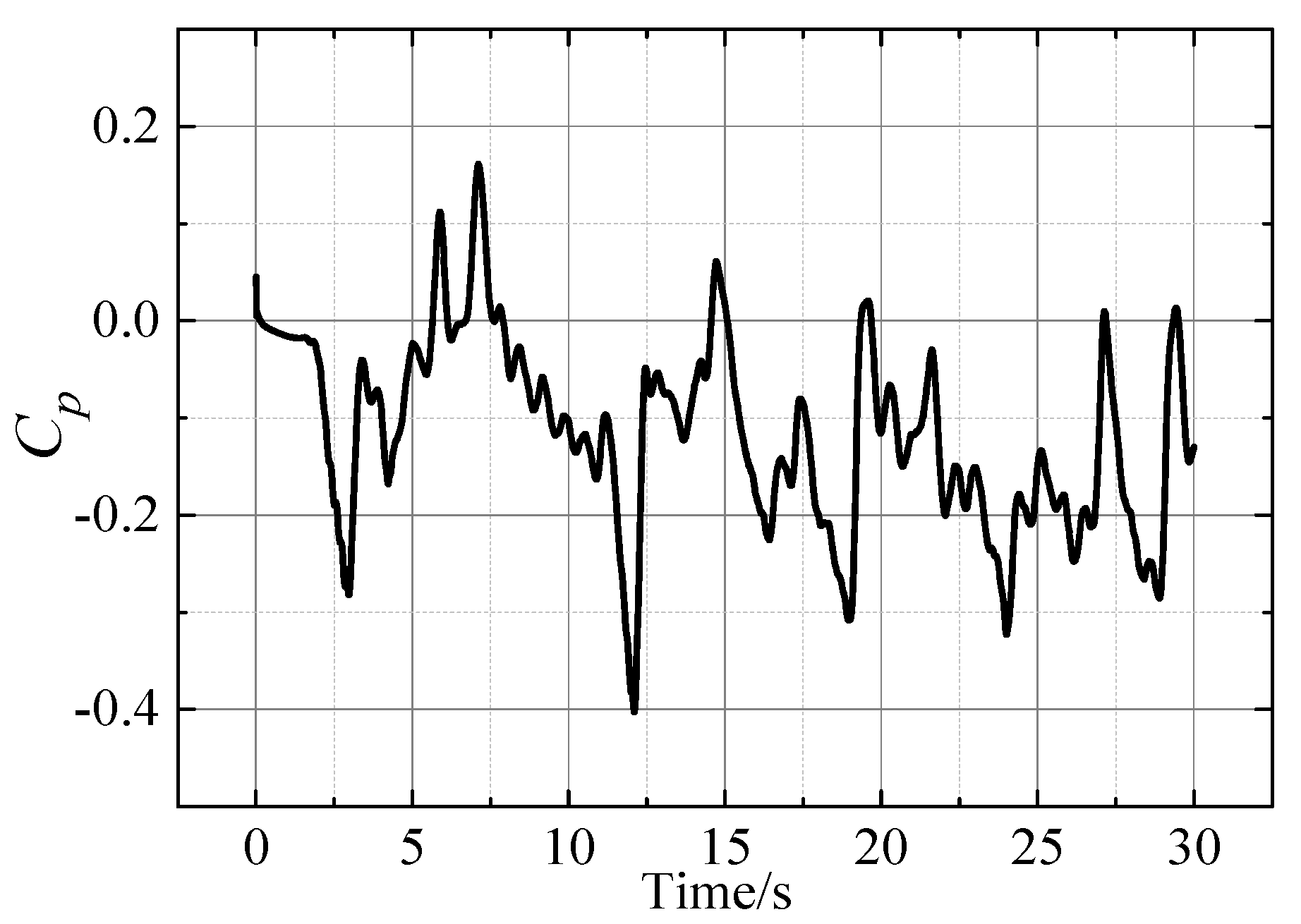
2. Flow Field Signal Acquisition

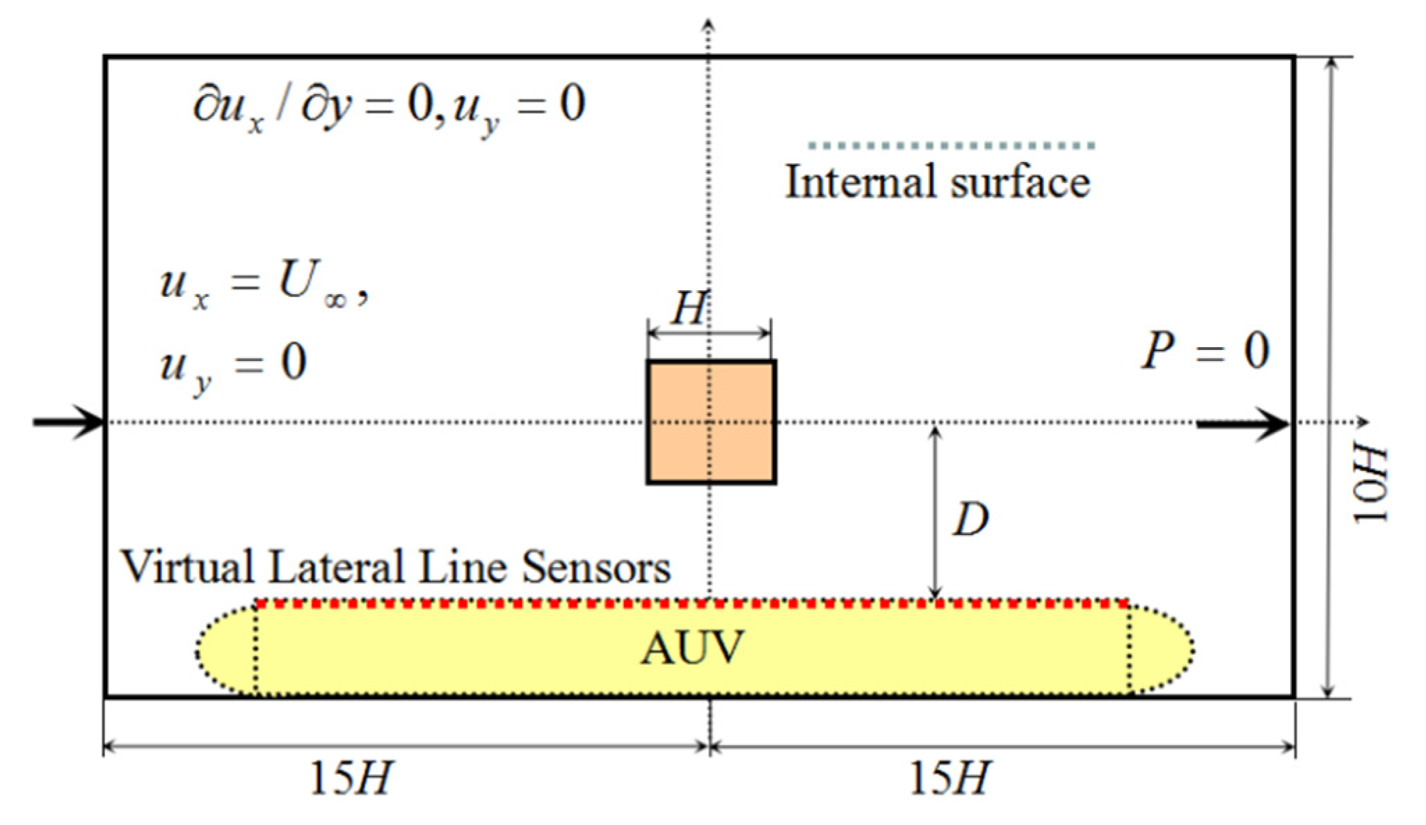
2.1. Numerical Scheme

In this paper, the flow field signal around a square target was chosen as the original signal, as shown in Figure 1. The side length of the square target was named $H$. The computational domain was located in a Cartesian coordinate system, within a range of $30H\times 10H$. The virtual lateral line with the pressure sensors was under the center of the targets at a distance of $D$. CFD was used to obtain the signal series, according to a numerical method described in our previous work [47].

In the numerical scheme, the two-step Taylor characteristic-based Galerkin (TCBG) method was used to solve the flow governing equation, which was presented by Bao et al. [48]. The progress of the TCBG scheme for the momentum equations is shown in flowing equations. The accuracy of the numerical scheme was validated previously [49]. The Strouhal numbers $S_t$ of the square target with different postures $\theta$ was computed, as shown in Figure 2. The results were in accord with previous reports, and the computational algorithm was adequate to solve the flow field around the underwater target.

$$u_i^{n+1/2}=u_i^n-\frac{\Delta t}{2}(u_j^n\frac{\partial u_i^n}{\partial x_j}+\frac{\partial p^n}{\partial x_i}-\frac{1}{Re}\frac{\partial {\tau }_{ij}^n}{\partial x_j})+\frac{\Delta t^2}{8}{u}_k^n\frac{\partial }{\partial x_k}(u_j^n\frac{\partial u_i^n}{\partial x_i}+2(\frac{\partial p^n}{\partial x_j}-\frac{1}{Re}\frac{\partial {\tau }_{ij}^n}{\partial x_j}))$$

(1)

$$u_i^{n+1}=u_i^n-\Delta t(u_j^{n+1/2}\frac{\partial u_i^n}{\partial x_j}+\frac{\partial p^{n+1}}{\partial x_i}-\frac{1}{Re}\frac{\partial {\tau }_{ij}^{n+1/2}}{\partial x_j})+\frac{\Delta t^2}{2}{u}_k^{n+1/2}\frac{\partial }{\partial x_k}(u_j^{n+1/2}\frac{\partial u_i^n}{\partial x_i}+\frac{\partial p^{n+1}}{\partial x_i}-\frac{1}{Re}\frac{\partial {\tau }_{ij}^{n+1/2}}{\partial x_j}))$$

(2)

$$\frac{{\partial }^2{p}^{n+1}}{\partial x_i\partial x_i}=\frac{1}{\Delta t}\frac{\partial }{\partial x_i}(u_i^n-u_i^{n+1})-\frac{\partial }{\partial x_i}(u_j^{n+1/2}\frac{\partial u_i^{n+1/2}}{\partial x_j}-\frac{1}{Re}\frac{\partial {\tau }_{ij}^{n+1/2}}{\partial x_j})$$

(3)

where $u_i$ is the i-component velocity, $\rho$ is the water density, $p$ is the pressure, ${\tau }_{ij}$ is the deviatoric stresses, $Re$ is the Reynolds number, $n$, $n+1/2$, and $n+1$ denote the time points of $t_n$, $t_{n+1/2}$ and $t_{n+1}$, respectively.

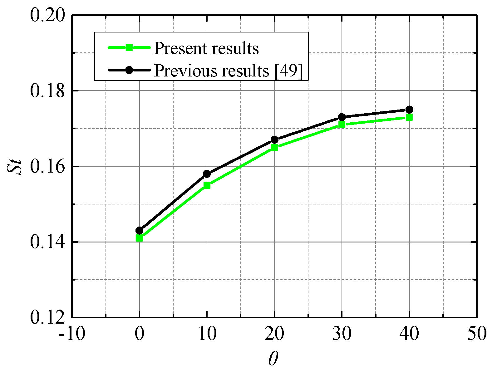
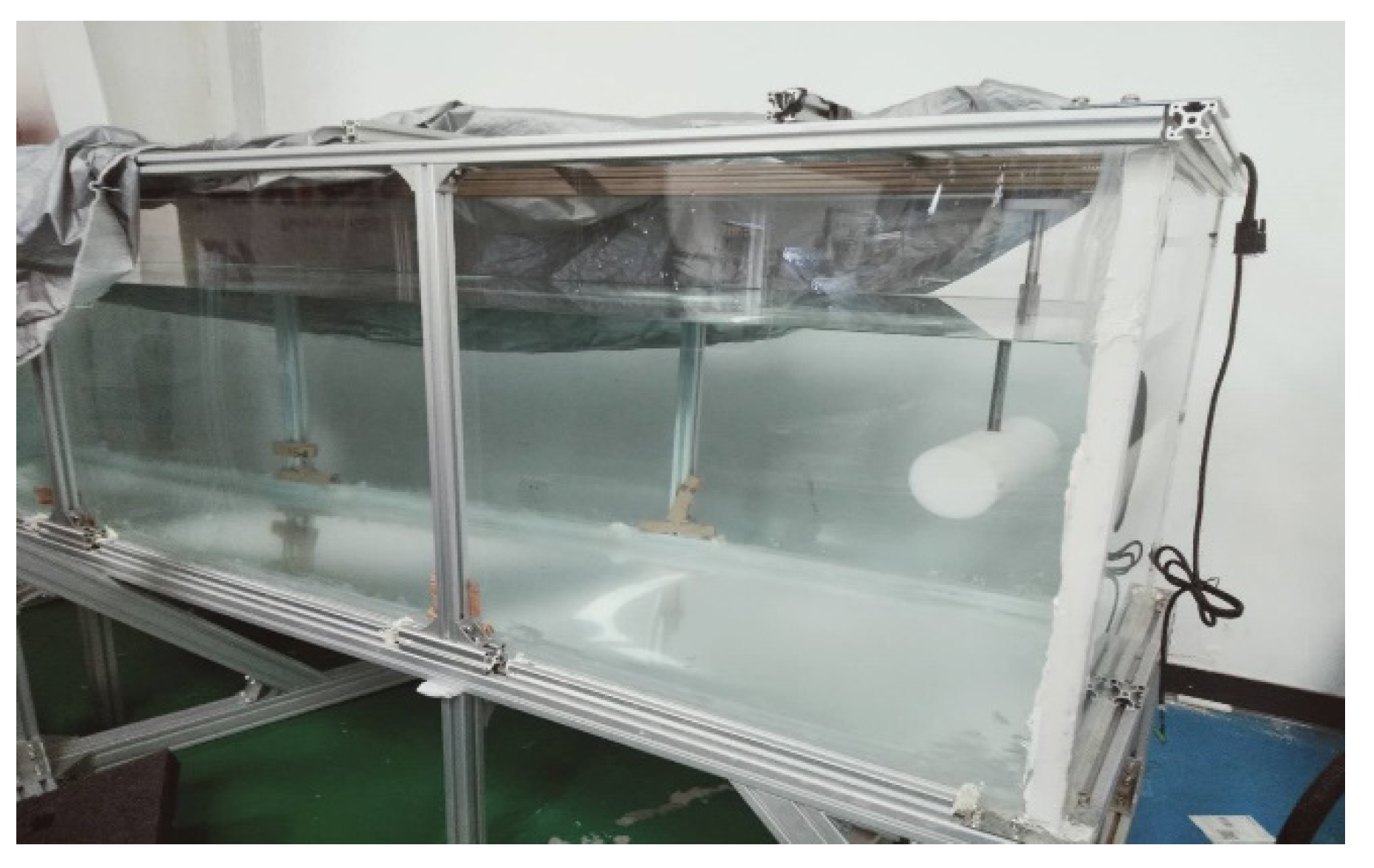
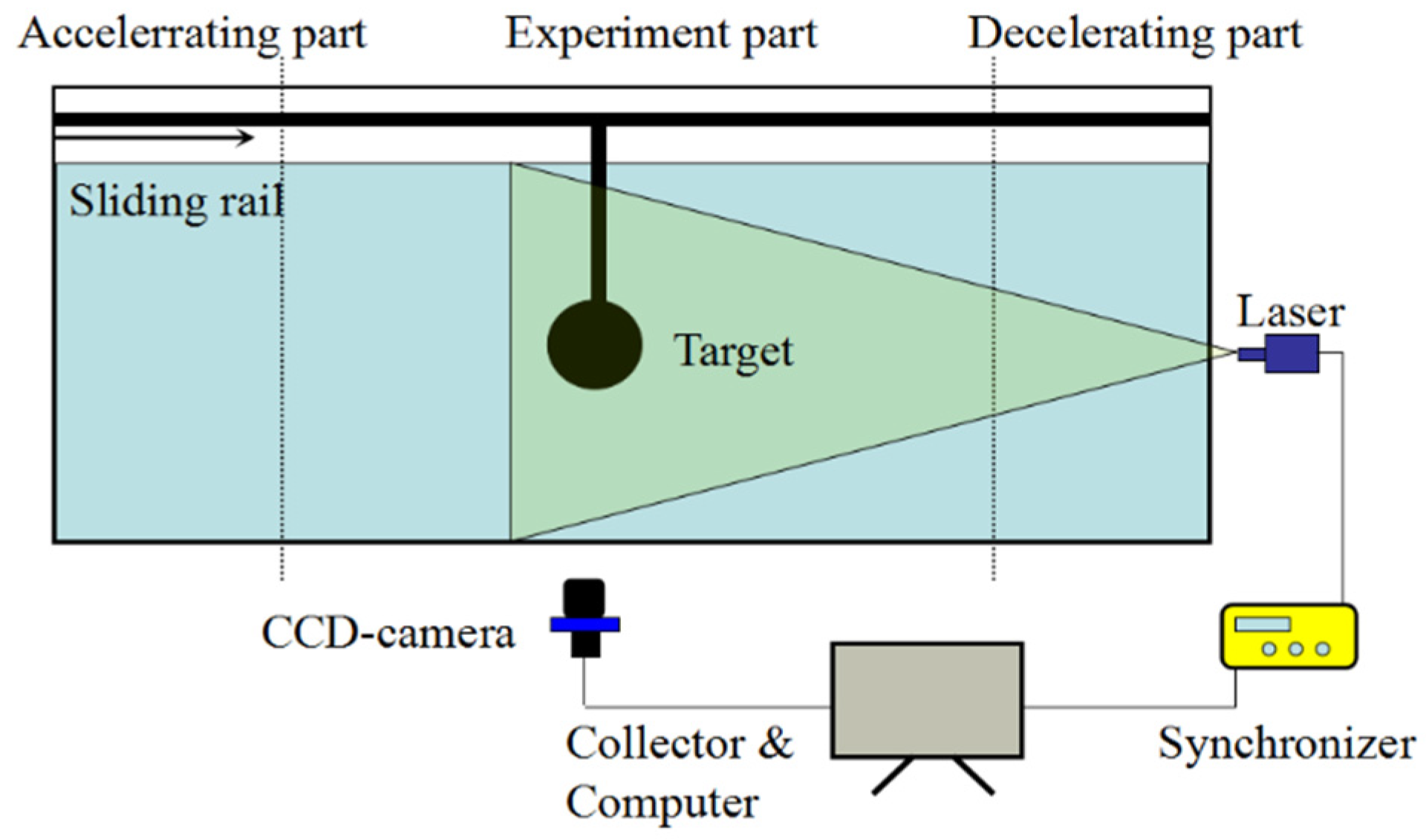
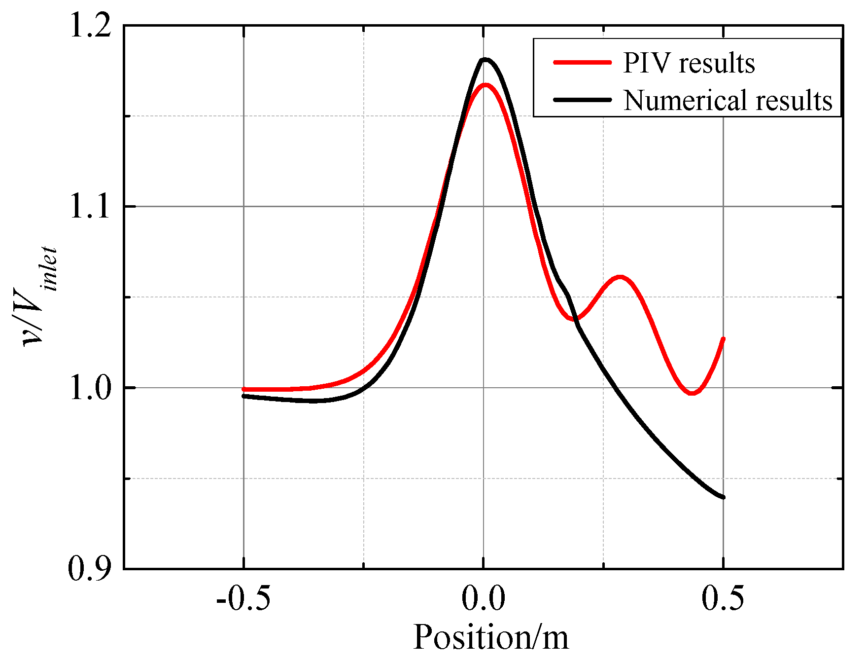
2.2. Numerical Validation by a PIV Experiment

A two-dimension PIV experiment was carried out to validate the numerical scheme. PIV is a method of visualizing the flow field based on an optical principle. Tracer particles with reflective properties are placed in the flow field. A laser emits a light source, and a high-speed camera is used to capture the motion path of the tracer particles along with the fluid. The displacement of the particles is calculated by the Fourier algorithm based on two successive frames of images, and the flow field structure is visualized. The experimental set is shown in Figure 3; the length of the water tank was 5.0 m, and its width and height were 1.0 m and 0.8 m, respectively. The water tank was divided into three parts: the accelerating part, the experiment part, and the decelerating part. The length of the experiment part was 3.0 m.

A sliding rail was used to make the target body move at a uniform speed, and the maximum speed was set at 1 m/s. As shown in Figure 4, the diameter of the target was 0.1 m, and its length was 0.2 m. The support point was located in the middle, and the distance between the center of the target and the bottom was 0.4 m. To ensure the original flow field was at rest, the experiments were carried out one by one, and the time interval between two adjacent experiments was 20 min.

The two-dimension PIV system was provided by TSI. The model of the layer was YAG200-NWL, with maximum output energy of 200 mJ, and its pulse width was 3–5 ns. The 4MX-CCD camera was used to capture the image of the flow field at 2048 × 2048 pixels. The minimum span frame time of the CCD camera was 200 ns, and its frame rate was 15 frames per second. In this experiment, images were collected in double-frame and double-exposure mode and processed by the mutual algorithm of the system. Some key parameters used in the experiment are shown in

Table 1. Some key parameters used in the PIV experiment.

Sampling Frequency/Hz	Sample Number	Laser Energy/mJ	Velocity Vector Number
100	300	100	256

.

The virtual LLS was set at a distance of 200 mm from the bottom. When the target moved to the middle of the experiment part, the axial velocity component $v_{x,//}$ of the virtual LLS was captured. The comparison between the experimental and the numerical results is shown in Figure 5. From it, we can see that the results of calculation and testing were in good agreement.

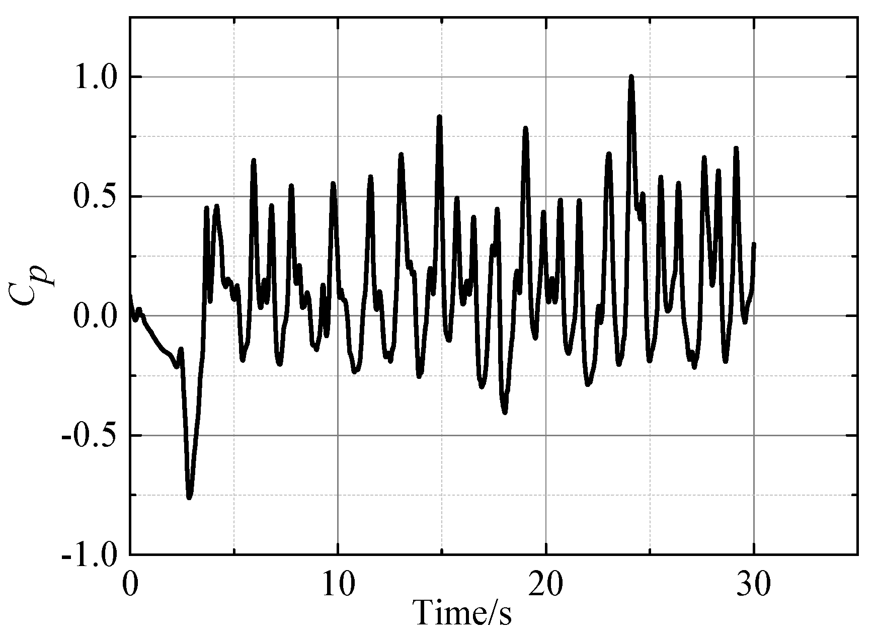
2.3. Phase Space Reconstruction

A virtual lateral line was set in the flow field, with 21 monitoring points. A weighting fusion algorithm was used to couple the 21-series signal, as described in our previous work [47] and shown in Equation (4).

$$\{\begin{array}{l}{K}_i=S_i+A_i\\ S_i=\frac{\epsilon \sin {\alpha }_i}{{\displaystyle \sum _{i=0}^N\sin {\alpha }_i}}\\ A_i=\frac{(1-\epsilon )A_m(s_i)}{{\displaystyle \sum _{i=0}^N{A}_m(s_i)}}\\ c_p(t)={\displaystyle \sum _{i=0}^N{K}_i{S}_i(t)}\end{array}$$

(4)

where $\epsilon$ is the weight of position coefficient $S_i$. $A_m(s_i)$ is the amplitude of signal collected by sensor $i$. $c_p(t)$ is the coupling signal series at the time of $t$.

In phase space reconstruction of the signal time series, the selection of delay time and embedding dimension was carried out by the C-C method, as shown in Equation (5). The first local minimum value times of $\Delta S(m,t)$ was considered the optimal delay time $\tau$. The minimum value of $S_{cor}(t)$ can be seen as the delay time window $\Gamma$, which has a connection with the embedding dimension $m$, as shown in Equation (5).

$$\begin{array}{l}\{\begin{array}{l}\overline{S}(t)=\frac{1}{16}{\displaystyle \sum _{m=2}^5{\displaystyle \sum _{j=1}^{4}S(m,r_j,t);}}\\ \Delta \overline{S}(t)=\frac{1}{4}{\displaystyle \sum _{m=2}^5\Delta S(m,t);}\\ S_{cor}(t)=\Delta \overline{S}(t)+\left|\Delta \overline{S}(t)\right|;\\ S(m,r_j,t)=\frac{1}{t}{\displaystyle \sum _{s=1}^t[C_s(m,r_j,t)-C_s^m(1,r_j,t)];}\\ \Delta S(m,t)=\max \left\{S(m,r_j,t)\right\}-\min \left\{S(m,r_j,t)\right\};\\ \Gamma =(m-1)\cdot \tau \end{array}\\ \end{array}$$

(5)

The final signal time series at high phase space $X_n(t_i)$ and the correlation integral $C(m,N,r,t)$ are shown in Equations (6) and (7). The pressure signal time series around a square target was defined as the original signal, as shown in Figure 6.

$$X_n(t_i)=[x_n(t_i),x_n(t_i+\tau ),x_n(t_i+2\tau ),\dots ,x_n(t_i+(m-1)\tau ],i=1,2,\dots ,N-(m-1)\tau$$

(6)

$$\{\begin{array}{l}C(m,N,r,t)=\frac{2}{M(M-1)}{\displaystyle \sum _{1\le i\le j\le M}\theta (r-d_{ij}),r>0}\\ d_{ij}=\left|X_n(t_i)-X_{n,}(t_j)\right|\end{array}$$

(7)

where $N$ is the length of the signal series, $r$ is the radius of the time series, $\sigma$ is the time-series standard deviation, $\theta (x)$ is shown in Equation (8).

$$\theta (x)=\{\begin{array}{l}0,x<0\\ 1,x>0\end{array}$$

(8)

3. Description of the Pretreatment Method

3.1. Description of the KKF-VSM

The signal time series obtained in Section 2 was processed by phase space reconstruction, as shown in Equation (6). If the flow field can be seen as a nonlinear system with a single input parameter $n\in Z^{+}\to x(n)$, where $n$ is the sample time, and $x(n)$ is the collected signal time series, the corresponding predicted signal $n\in Z^{+}\to y(n)$ is single and can be expressed by the VSM, as shown in Equation (9). The output of the system can be divided into linear and nonlinear parts [50], as shown in Equation (10).

If the length of the expanded series is too big, this method is not easy to converge. It is necessary to minimize the length to ensure prediction accuracy. Therefore, the Kautz function was used to expand the Volterra series, as shown in Equation (11). It can predict the response of a nonlinear system and monitor the structure of interest [51,52].

$$y(n)={\displaystyle \sum _{p=1}^{\infty }{\displaystyle \sum _{m_1}^{N_1-1}\dots {\displaystyle \sum _{m_p=0}^{N_p-1}{h}_p(m_1,\dots ,m_p)}}}{\displaystyle \prod _{i=1}^{p}u(n-m_i)}$$

(9)

$$y(n)=\underset{linear}{\underbrace{y_1(n)}}+\underset{nonlinear}{\underbrace{y_2(n)+y_3(n)+\dots +y_p(n)}}$$

(10)

$$h_p(m_1,\dots ,m_p)\approx {\displaystyle \sum _{i_1=1}^{J_1}\dots {\displaystyle \sum _{i_p=1}^{J_p}{\Re }_p(i_1,\dots ,i_p){\displaystyle \prod _{j=1}^p{\Psi }_{p,i_j}(m_j)}}}$$

(11)

where $h_p(m_1,\dots ,m_p)$ is the p-order Volterra kernel, $J_{1,\dots \dots ,}{J}_p$ is the number of Kautz functions used in each orthonormal projections of the Volterra kernels, ${\Re }_p(i_1,\dots ,i_p)$ is the p-order Volterra kernel expanded in the orthonormal basis, ${\Psi }_{p,i_j(m_j)}$ is the i-th Kautz filter, which is shown in Equation (12).

$$\{\begin{array}{l}{\Psi }_{p,2j}(z)={\Psi }_{p,2j-1}(z)\frac{z-b_p}{\sqrt{1-b_p^2}}\\ {\Psi }_{p,2j-1}(z)=\frac{z\sqrt{(1-b_p^2)(1-c_p^2)}}{z^2+b_p(c_p-1)z-c_p}{[\frac{-c_p{z}^2+b_p(c_p-1)z+1}{z^2+b_p(c_p-1)z-c_p}]}^{j-1}\\ b_p=\frac{{\Gamma }_p+{\tilde{\Gamma }}_p}{1+{\Gamma }_p{\tilde{\Gamma }}_p}\\ c_p=-{\Gamma }_p{\tilde{\Gamma }}_p\\ {\Gamma }_p=\exp (\frac{S_p}{F_s})\\ S_p=-{\xi }_p{\omega }_p\pm j{\omega }_p\sqrt{1-{\xi }_p^2}\end{array}$$

(12)

where ${\omega }_p$ is the natural frequency of the system, ${\xi }_p$ is the damping ratio of the flow field, $F_s$ is the sampling frequency, $S_p$ is the continuous poles of the input signal series, $\Gamma$ and $\tilde{\Gamma }$ are the Kautz poles and its complex conjugate in the discrete domain.

The steps for predicting the flow field signal based on the KKF-VSM were as follows:

1.

Establish a reference system: the known signal series was used to train the KKF-VSM, as the reference system;

2.

Input the test series: the test signal series $x_n=[x(1),x(2),\dots ,x(N)]$ was normalized by Equation (13), and Equation (14) was used to establish the input signal matrix;

$$x^{*}(n)=\frac{x(n)-\frac{1}{N}{\displaystyle \sum _{i=1}^{N}x(i)}}{\max (x(n))-\min (x(n))}$$

(13)

$$X(n)=\left[\begin{array}{cccc}{x}^{*}(1)& x^{*}(2)& \cdots & x^{*}(N-(m-1))\\ x^{*}(2)& x^{*}(3)& \cdots & x^{*}(N-(m-2))\\ ⋮& ⋮& & ⋮\\ x^{*}(m)& x^{*}(m+1)& \cdots & x^{*}(N)\end{array}\right]$$

(14)

where $x^{*}(n)$ is the processed data, $x(n)$ is the original data, $\min (x(n))$ and $\max (x(n))$ respects the minimum and maximum values of the original signal.

3.

Phase space reconstruction: the input signal matrix was reconstructed in higher phase space, and the signal matrix $U(n)$ to the input into the KKF-VSM was obtained;

4.

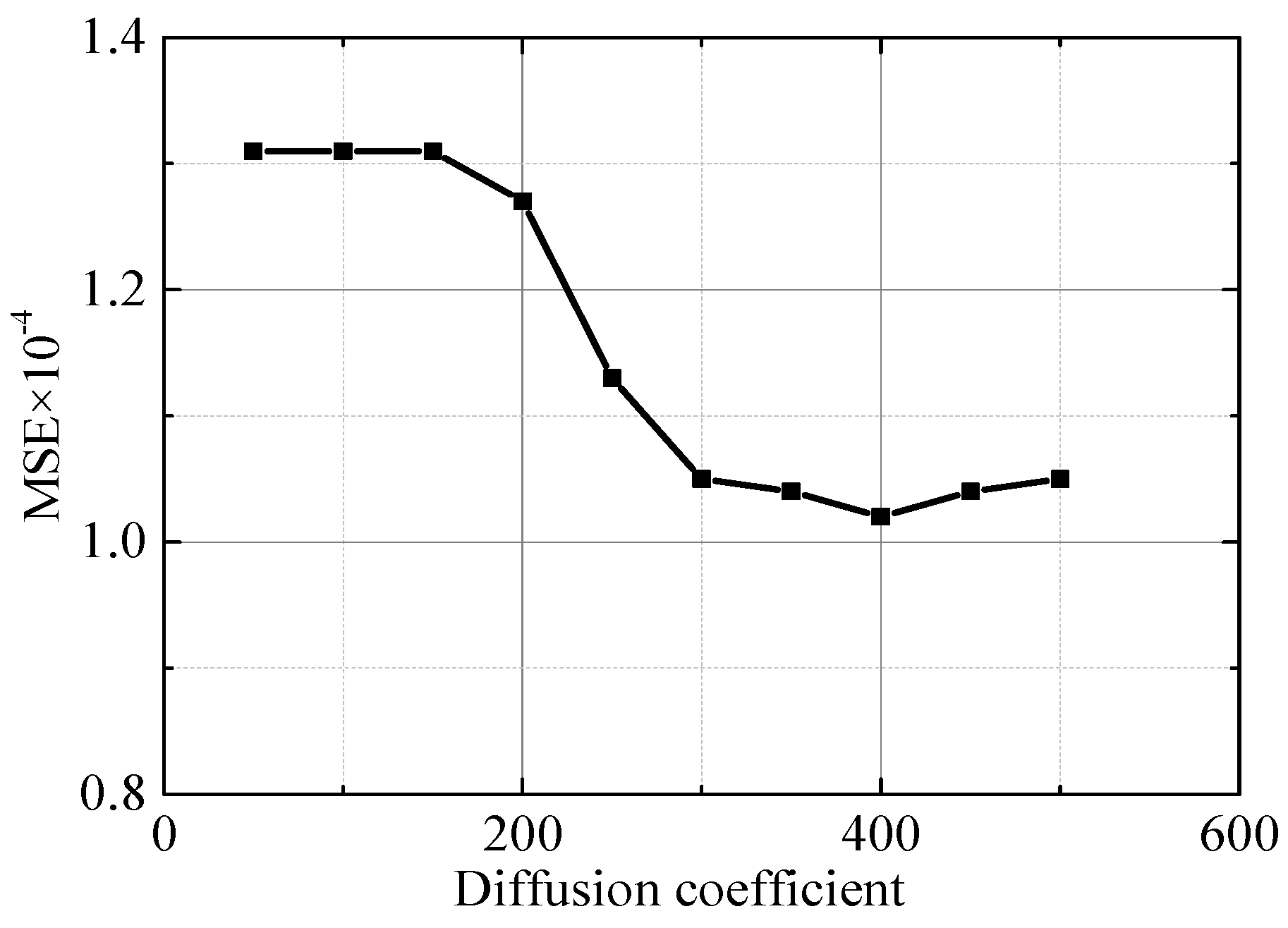
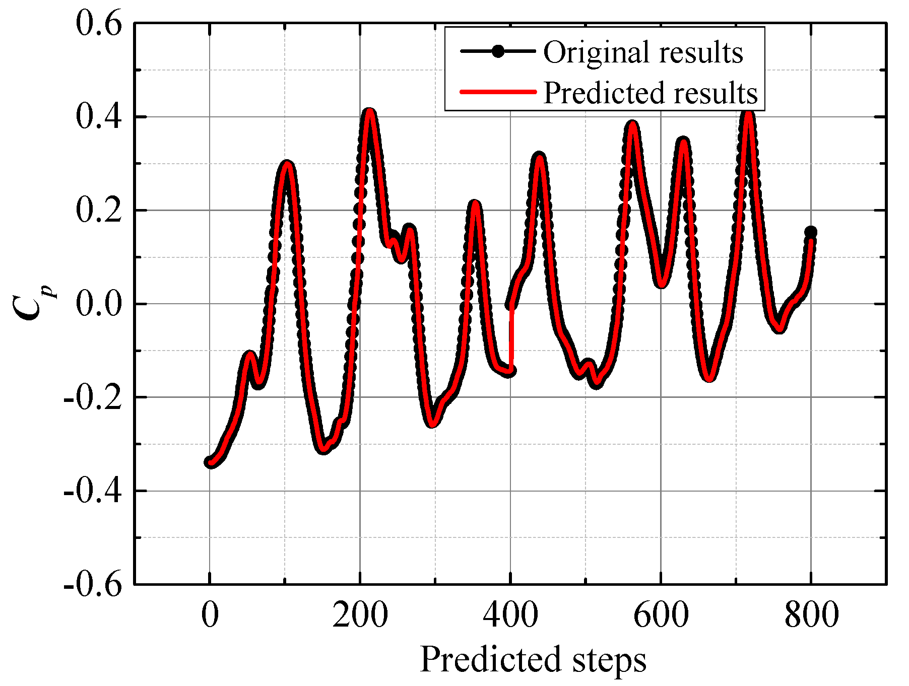
Sample prediction test: the KKF-VSM was used to obtain the output of the sample series, consisting of the orthonormal kernels and the input signal, as shown in Equation (15). The prediction error was expressed as the mean-square error (MSE), as shown in Equation (16).

$$y(n)\approx {\displaystyle \sum _{p=1}^{\infty }{\displaystyle \sum _{i_1=1}^{J_1}\dots {\displaystyle \sum _{i_p=1}^{J_p}{\Re }_p(i_1,\dots ,i_p){\displaystyle \prod _{j=1}^p{\displaystyle \sum _{m_i=0}^{J_{\max }}{\Psi }_{p,i_j}(m_j)}}}}}u(n-m_i)$$

(15)

$$MSE=\frac{{\displaystyle \sum _{n=1}^N{[x(n)-y(n)]}^2}}{N}$$

(16)

The maximum number of samples was set as to. During the training process, KKF-VSM was trained with 2200 samples, and the other 800 samples were used in the test. When the delay time $\tau$ was 27 and the embedding dimension was 7, one-order, two-order, and three-order KKF-VSM was used to predict the samples. The predicting steps corresponded to the sample time $n$, and the results are shown in Figure 7, Figure 8 and Figure 9.

The MSE of the three models is shown in Figure 7. From it, it appears that the MSE obviously changed from one-order KKF-VSM to two-order KKF-VSM. The change was slower when comparing two-order to three-order KKF-VSM. This implies that the contribution of the two-order component was the largest in this test sample. The third-order component could correct some specific values to fit the trend. As a result, three-order KKF-VSM was chosen in this paper to ensure predicting accuracy.

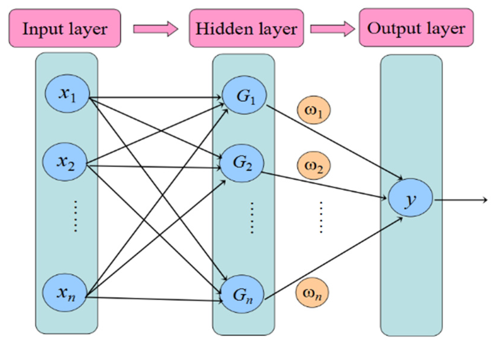
3.2. Description of the RBF-NNM

The RBF-NNM was a three-layer forward network, as shown in Figure 10. Through the radial basis function in each hidden layer, the input signal $X(n)$ can find the optimal fitting plane in multidimensional space. Therefore, the RBF-NNM provides a good fit in the prediction of a chaotic signal time series.

The Gaussian kernel function is normally used in the RBF-NNM, as shown in Equation (17); the output $y(n)$ is shown in Equation (18).

$$G_i(X)=\exp \left[-\frac{{\Vert X-C_i\Vert }^2}{2{\sigma }_i^2}\right],i=1,2,\cdots ,m$$

(17)

$$y(n)={\displaystyle \sum _{i=1}^m{\omega }_i{G}_i(X)}$$

(18)

where $X$ is the m-dimension input matrix, $C_i$ is the center of the i-th basis function, ${\sigma }_i$ is the width of the i-th hidden node, $m$ is the number of the perceivable unit, ${\omega }_i$ is the connection weight from the i-th hidden layer to the output.

The above parameters can be obtained by using the K-means clustering algorithm, as follows:

1.

Determine the cluster center: first, some clustering centers were determined randomly and defined as $c_i(i=1,2,\cdots ,h)$. The training samples $x_j$ were allocated to each cluster set $v_j(j=1,2,\cdots ,P)$, based on the principle of minimizing the Euclidean distance between the training samples and the clustering center. The samples average in each set was iterated, and the result was defined as the new cluster center $c_i$. Repeat the calculation cycle until the residual was less than the setting value and use the final $c_i$ as the cluster center of the basis function;

2.

Determine the width of the hidden node: the maximum $c_{i,\max }$ was chosen from the cluster center set, and the width of the hidden node can be solved by Equation (19);

$${\sigma }_i=\frac{c_{i,\max }}{\sqrt{2h}},(i=1,2,\cdots ,h)$$

(19)

3.

Determine the connection weights: the least-square method was used to calculate the weight, as shown in Equation (20).

$${\omega }_i=\exp (\frac{h}{c_{i,\max }^2}{\Vert x_j-c_i\Vert }^2),(i=1,2,\cdots ,h;j=1,2,\cdots ,P)$$

(20)

The training epoch $N_q$ and the testing epoch $N_p$ in Section 2.1 were used to build the RBF-NNM. The diffusion coefficient $s$ of RBF was analyzed, and the optimum value was chosen. Commonly, the fitting radial basis function is smoother when $s$ is larger, but if it is larger than a critical value, some numerical problem will appear. As seen in Figure 11, $s$ was optimized in the range from 50 to 500, and when it was 400, the MSE was at its minimum. Therefore, in the following analysis, the diffusion coefficient was set to 400.

The RBF-NNM was used to predict the trend of the signal sample, as shown in Figure 12. From it, it appeared that the RBF-NNM can also predict the changing trend of the flow field signal.

4. Comparative Analysis Results

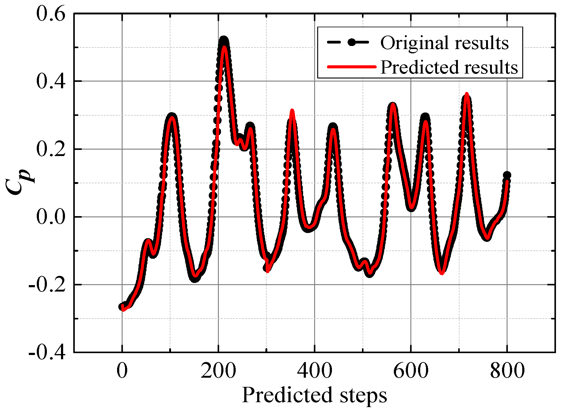
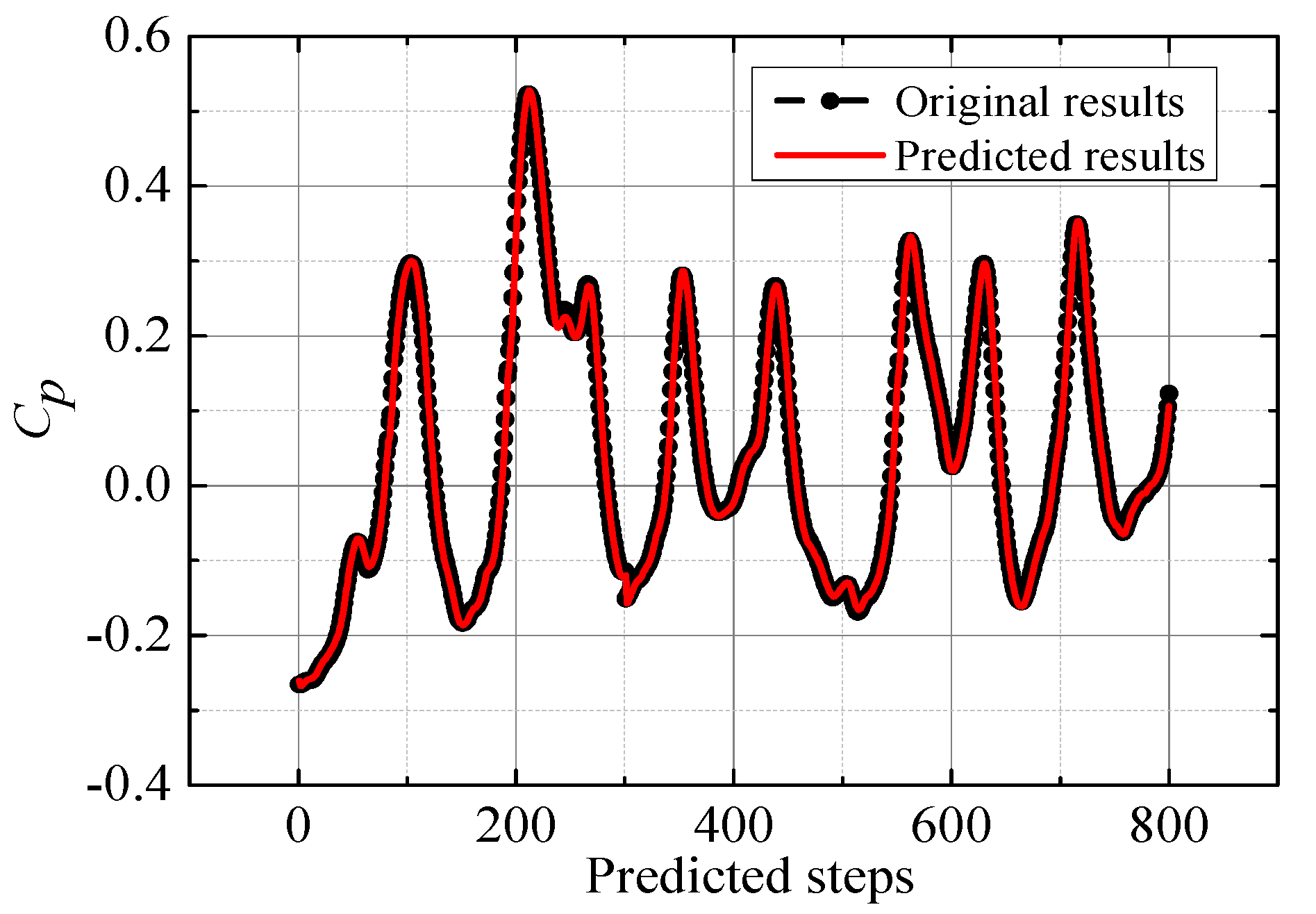
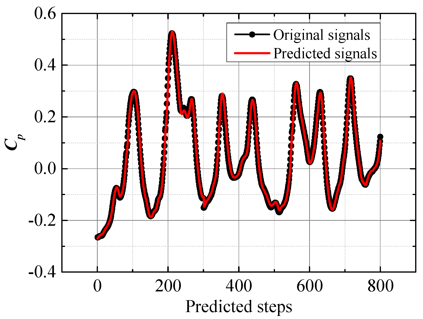
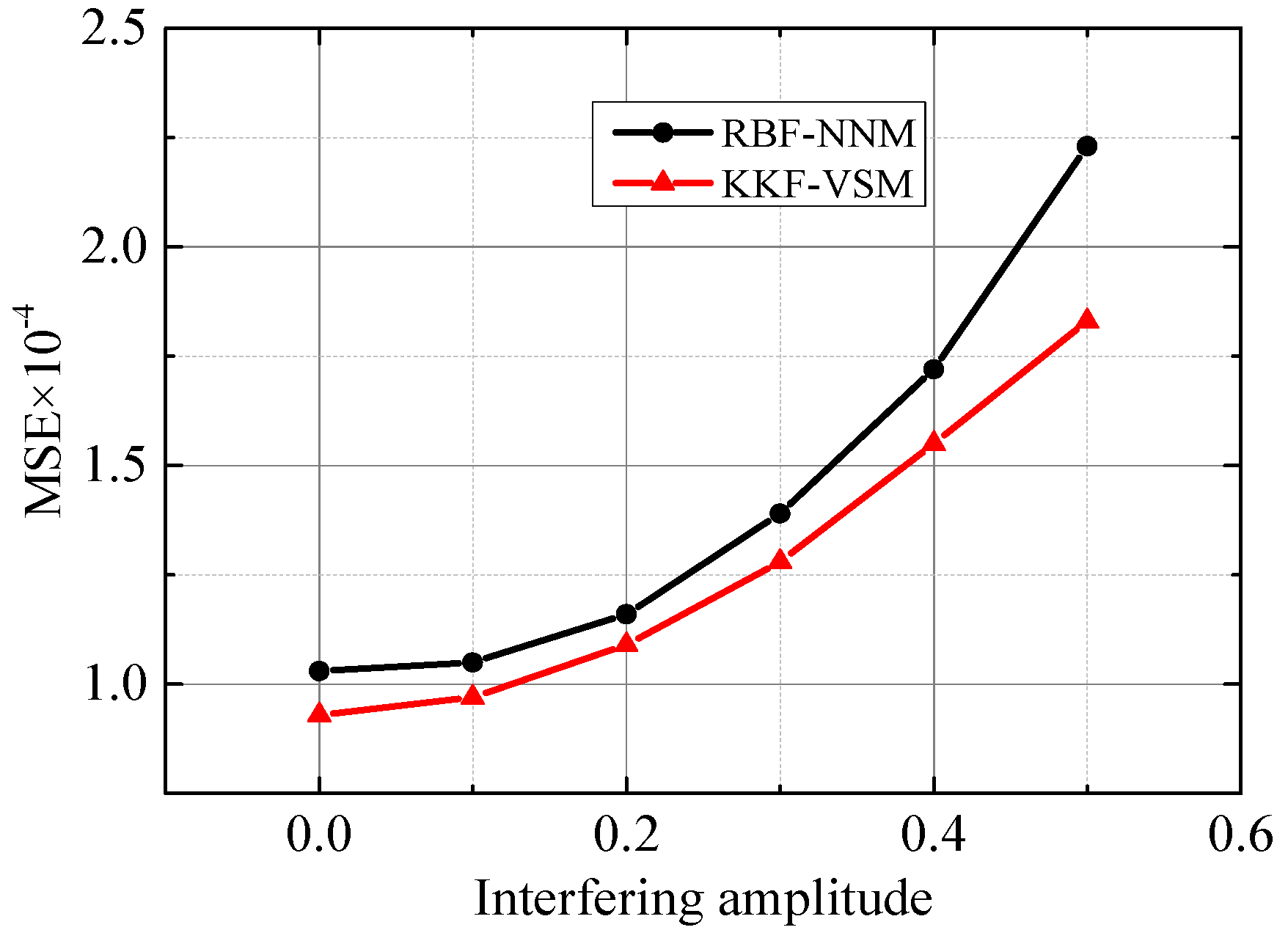
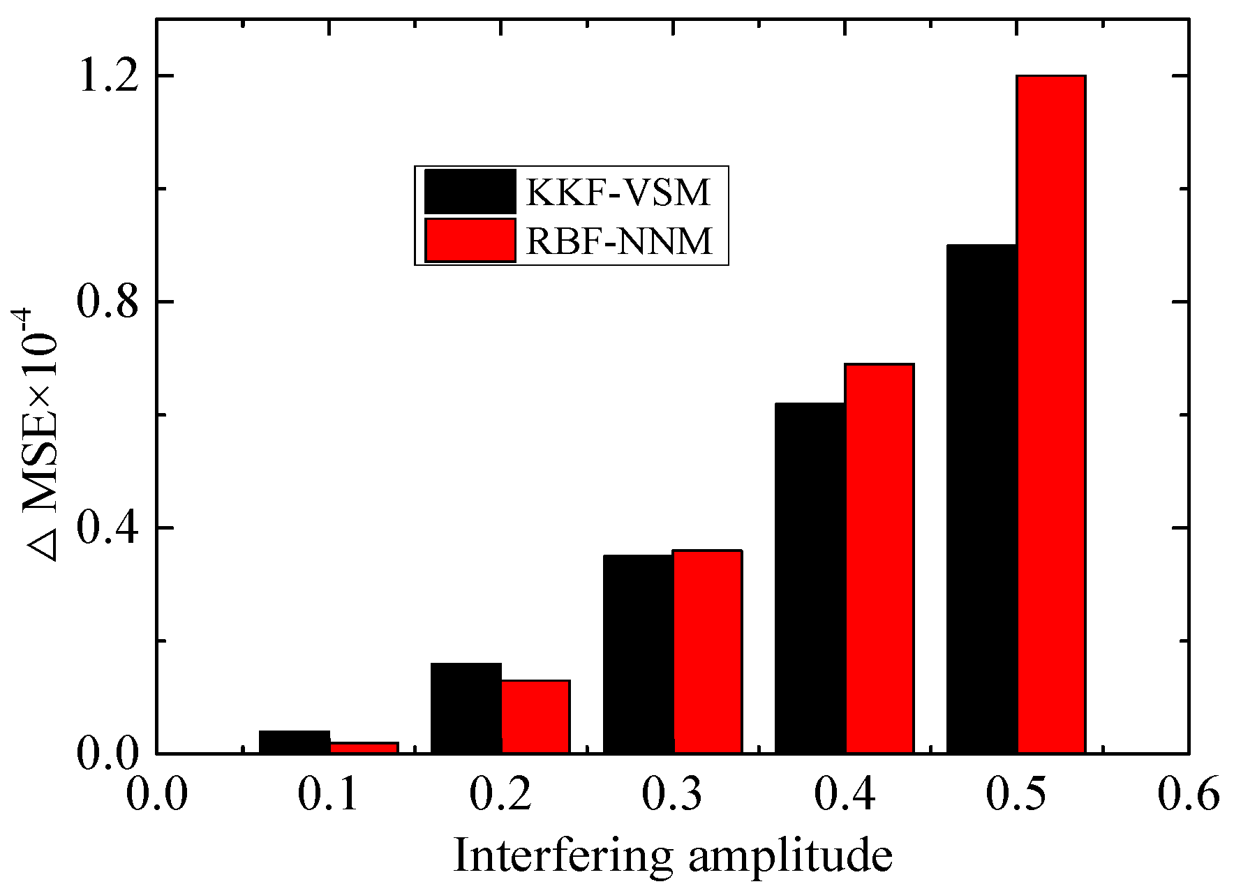
4.1. Analysis of Regular Undesired Signals

In the natural underwater environment, there are interference factors, such as ocean currents, shock waves, and surrounding objects. An approximate mathematical model describing these factors was built, and the KKF-VSM and RBF-NNM were compared when processing the signal time series.

First, the interference of a regular wave on the flow field signal was analyzed. From the first to 400th value of the original test samples, one regular undesired signal series $S(n)$ with a sine wave was put in, as shown in Equation (21). The three-order KKF-VSM and RBF-NNM were used to filter the undesired signal and predict the original test samples. The variation curve of MSE with the amplitude of $S(n)$ is shown in Figure 13.

$$S(n)=A\sin (\frac{n\pi }{4}),n=1,2,\cdots ,500$$

(21)

where $S(n)$ is the interfering signal series with the sine wave, and $A$ is the amplitude.

As seen in Figure 13, when the strength of undesired signals was the same, the MSE of KKF-VSM was smaller than that of RBF-NNM. In addition, the gradient of the KKF-VSM curve was also smaller than that of the RBF-NNM one. These results imply that the robustness of RBF-NNM was poor when the undesired signals were strong. In comparison, the KKF-VSM showed a more robust performance because KKF-VSM contained both the linear and the nonlinear components at the same time.

When the order of KKF-VSM changed, the contribution of each part to the method’s robustness was analyzed, as shown in

Table 2. Influence of Volterra orders on the robustness.

$\mathbf{Amplitude}/\mathit{A}$	0.1	0.2	0.3	0.4	0.5
$MS{E}_{1-\mathrm{order}}\times {10}^{-3}$	1.94	2.43	3.17	4.29	5.87
$MS{E}_{2-\mathrm{orders}}\times {10}^{-4}$	1.46	1.77	2.27	2.97	3.84
$MS{E}_{3-\mathrm{orders}}\times {10}^{-4}$	0.97	1.09	1.28	1.55	1.83

. From it, we can see that MSE decreased when KKF-VSM changed from one order to two orders. That implies the second component of KKF-VSM could express the most nonlinear characteristic of the test sample. Furthermore, when the KKF-VSM changed from two orders to three orders, the gradient of MSE obviously decreased, implying that the three-order component provided a clear contribution to the robustness.

The sensitivity of KKF-VSM and RBF-NNM to regular undesired signals was compared. The results are shown in Figure 14. From it, it appears that when the amplitude of undesired signals was small, the $\Delta MSE$ in KKF-VSM changed more obviously than that in RBF-NNM, but the result was the opposite when the amplitude became larger. This phenomenon implies that KKF-VSM can capture weak interference signals more easily than RBF-NNM; in other words, KKF-VSM has a greater ability to filter regular undesired signals than RBF-NNM.

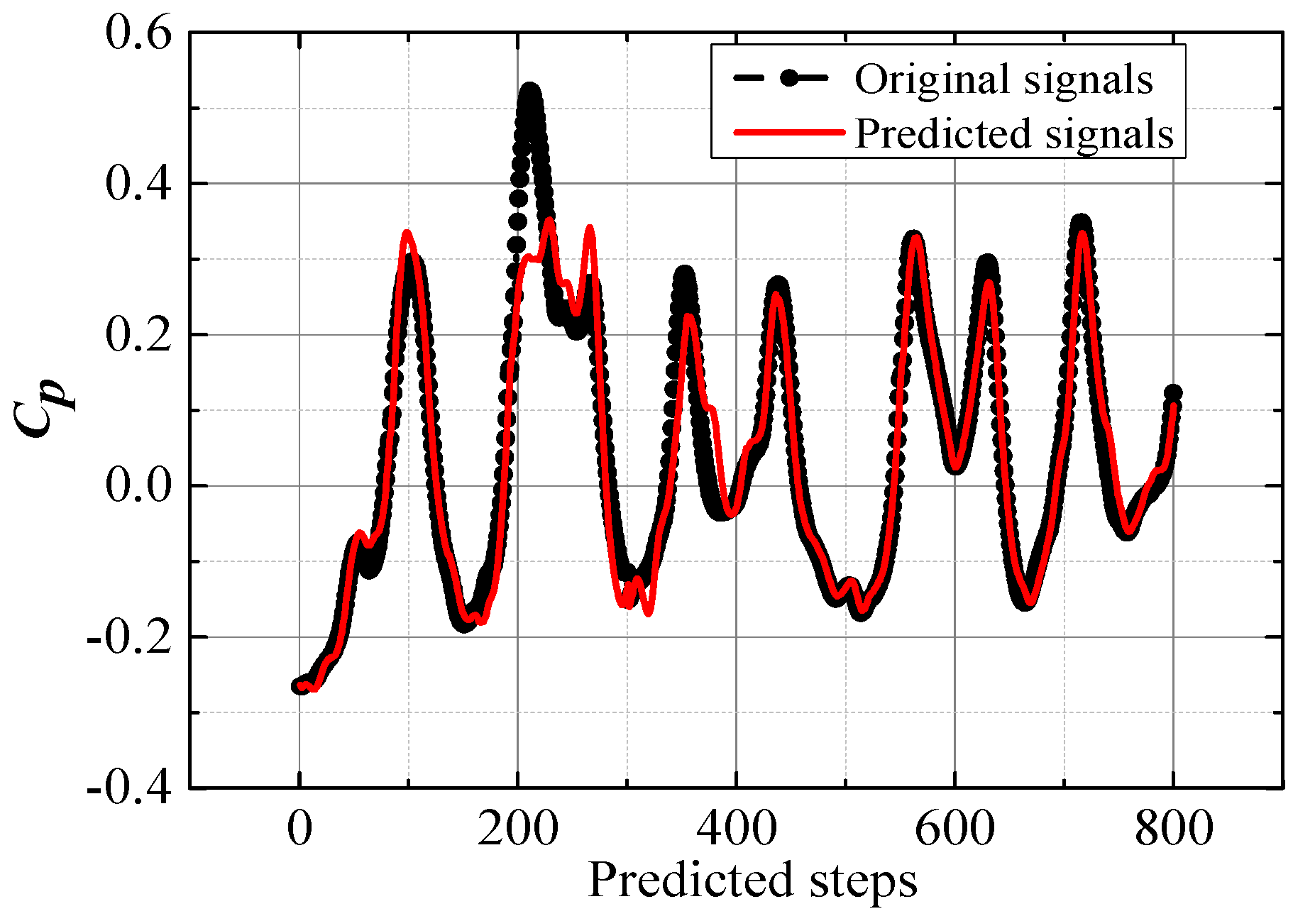
4.2. Analysis of Irregular Undesired Signals

If there is an obstacle near the target in the flow field, it will have an impact on the original signal, and the undesired signal is usually chaotic. In this paper, the flow field around a triangle obstacle was used as an irregular undesired signal, as shown in Figure 15. Noise was added in correspondence of the regular undesired signal by linear superposition into the original test sample, as shown in Equation (22).

$$\chi (n)=\{\begin{array}{l}x(n),1\le n\le 2200\\ x(n)+T(n),2201\le n\le 2400\\ x(n),2401\le n\le 3000\end{array}$$

(22)

where $x(n)$ is the original signal, $T(n)$ is the undesired signal, $\chi (n)$ is the final testing original signal series.

The KKF-VSM and RBF-NNM were used to filter the irregular undesired signal and predict the original test sample. The results are shown in Figure 16 and Figure 17. The results indicated that the irregular undesired signal could be filtered, and the change trend of the original samples could be predicted very well by both models. Furthermore, the MSE of RBF-NNM was $1.625\times {10}^{-4}$, and that of three-order KKF-VSM was $1.374\times {10}^{-4}$. That indicated that the robustness of the three-order KKF-VSM is higher than that of RBF-NNM.

5. Conclusions

In order to estimate the flow field signal change based on the flow sensing mechanism of a lateral line system, so to improve the environment adaptability of AUVs, a novel KKF-VSM was provided, using the Kautz function as the kernel function. This is a novelty compared to previous related works, which were mainly based on RBF-NNM, and VSM with the frequency response function as the kernel function. The flow field around a square target was studied, and its pressure signal time series was obtained by CFD and PIV. The predicting accuracy, sensitivity, and robustness of KKF-VSM were analyzed in this work. In addition, an RBF-NNM with a Gaussian kernel function was compared with KKF-VSM. Some interesting conclusions were made. The pressure signal of the flow field around the square target was chaotic, and KKF-VSM and RBF-NNM could predict its change trend very well. However, in comparison with RBF-NNM, KKF-VSM showed higher accuracy in filtering regular and irregular noise. Furthermore, KKF-VSM appeared to capture weak undesired signals more easily, and its filter ability was more robust than that of RBF-NNM. In future work, the authors intend to apply this procedure considering an experimental setup in a natural underwater environment.

References

1. Yu, J.C.; Sun, C.Y.; Zhang, A.Q. The Present Status of Environmental Energy Harvesting and Utilization Technology of Marine Robots. Robot 2018, 40, 89–101. [Google Scholar]
2. Feng, X.; Li, Y. Thirty years evolution of SIA’s unmanned marine vehicle. Chin. Sci. Bull. 2013, 58, 2–7. [Google Scholar] [CrossRef]
3. Lu, W.; Liu, D. A Frequency-Limited Adaptive Controller for Underwater Vehicle-Manipulator Systems Under Large Wave Disturbances. In Proceedings of the 13th World Congress on Intelligent Control and Automation (WCICA), Changsha, China, 4–8 July 2018. [Google Scholar]
4. Sarhadi, P.; Noei, A.R.; Khosravi, A. Model reference adaptive PID control with anti-windup compensator for an autonomous underwater vehicle. Robot. Auton. Syst. 2016, 83, 87–93. [Google Scholar] [CrossRef]
5. Rout, R.; Subudhi, B. Inverse optimal self-tuning PID control design for an autonomous underwater vehicle. Int. J. Syst. Sci. 2016, 48, 367–375. [Google Scholar] [CrossRef]
6. Santos, C.H.F.; Cildoz, M.U.; Terra, M.H.; Pieri, E.R.D. Backstepping Sliding Mode Control with Functional Tuning Based on an Instantaneous Power Approach Applied to an Underwater Vehicle. Int. J. Syst. Sci. 2018, 49, 859–867. [Google Scholar] [CrossRef]
7. Li, J.-H.; Kim, M.-G.; Kang, H.; Lee, M.-J.; Cho, G.R. UUV Simulation Modeling and its Control Method: Simulation and Experimental Studies. J. Mar. Sci. Eng. 2019, 7, 89. [Google Scholar] [CrossRef] [Green Version]
8. Teixeira, M.A.S.; Dalmedico, N.; Santos, H.B.; Oliveira, A.S.D.; Arruda, L.V.R.D.; Neves, F. Enhancing Robot Capabilities of Environmental Perception Through Embedded GPU. In Proceedings of the 2017 VII Brazilian Symposium on Computing Systems Engineering (SBESC), Curitiba, Brazil, 6–10 November 2017. [Google Scholar]
9. Ferri, G.; Munafo, A.; LePage, K.D. An Autonomous Underwater Vehicle Data-Driven Control Strategy for Target Tracking. IEEE J. Ocean. Eng. 2018, 43, 323–343. [Google Scholar] [CrossRef]
10. Huma, G.; Youngtae, N. An Overview of Next-Generation Underwater Target Detection and Tracking: An Integrated Underwater Architecture. IEEE Access 2019, 7, 99. [Google Scholar]
11. Emberton, S.; Chittka, L.; Cavallaro, A. Underwater image and video dehazing with pure haze region segmentation. Comput. Vis. Image Underst. 2018, 168, 145–156. [Google Scholar] [CrossRef]
12. Li, C.; Guo, J. Underwater image enhancement by dehazing and color correction. J. Electron. Imaging 2015, 24, 033023. [Google Scholar] [CrossRef]
13. Zhang, J.X. Principle of Biomimetic Detection Based on Flow Field Information of Underwater Moving Object. Master’s Thesis, Beijing Institute of Technology, Beijing, China, 2015. [Google Scholar]
14. Laura, R.; Abbate, F.; Germanà, G.P.; Montalbano, G.; Germana, A.; Levanti, M. Fine structure of the canal neuromasts of the lateral line system in the adult zebrafish. Anat. Histol. Embryol. 2018, 47, 322–329. [Google Scholar] [CrossRef]
15. Abbate, F.; Madrigrano, M.; Scopitteri, T.; Levanti, M.; Cobo, J.; Germanà, A.; Vega, J.; Laurà, R. Acid-sensing ion channel immunoreactivities in the cephalic neuromasts of adult zebrafish. Ann. Anat. 2016, 207, 27–31. [Google Scholar] [CrossRef]
16. Baxendale, S.; Whitfield, T. Methods to study the development, anatomy, and function of the zebrafish inner ear across the life course. Methods Cell Biol. 2016, 134, 165–209. [Google Scholar] [CrossRef] [PubMed]
17. Jiang, Y.; Fu, J.; Zhang, D.; Zhao, Y. Investigation on the lateral line systems of two cavefish: Sinocyclocheilus Macrophthalmus and Microphthalmus (Cypriniformes: Cyprinidae). J. Bionic Eng. 2016, 13, 108–114. [Google Scholar] [CrossRef]
18. Becker, E.A.; Bird, N.C.; Webb, J.F. Post-embryonic development of canal and superficial neuromasts and the generation of two cranial lateral line phenotypes. J. Morphol. 2016, 277, 1273–1291. [Google Scholar] [CrossRef]
19. Angelo, D.L.; Lossi, L.; Merighi, A.; Girolamo, P.D. Anatomical Features for the Adequate Choice of Experimental Animal Models in Biomedicine: I. Fishes. Ann. Anat. 2016, 205, 75–84. [Google Scholar] [PubMed]
20. Cruz, I.A.; Kappedal, R.; Mackenzie, S.M.; Hailey, D.W.; Hoffman, T.L.; Schilling, T.F.; Raible, D.W. Robust regeneration of adult zebrafish lateral line hair cells reflects continued precursor pool maintenance. Dev. Biol. 2015, 402, 229–238. [Google Scholar] [CrossRef] [Green Version]
21. Butler, J.M.; Maruska, K.P. The mechanosensory lateral line is used to assess opponents and mediate aggressive behaviors during territorial interactions in an African cichlid fish. J. Exp. Biol. 2015, 218, 3284–3294. [Google Scholar] [CrossRef] [PubMed] [Green Version]
22. Yoshizawa, M.; Jeffery, W.R.; van Netten, S.M.; McHenry, M.J. The sensitivity of lateral line receptors and their role in the behavior of Mexican blind cavefish (Astyanax mexicanus). J. Exp. Biol. 2013, 217, 886–895. [Google Scholar] [CrossRef] [Green Version]
23. Abdulsadda, A.; Tan, X. An artificial lateral line system using IPMC sensor arrays. Int. J. Smart Nano Mater. 2012, 3, 226–242. [Google Scholar] [CrossRef] [Green Version]
24. Reida, A.; Windmilla, J.F.C.; Uttamchandani, D. Bio-inspired Sound Localization Sensor with High Directional Sensitivity. Procedia Eng. 2015, 120, 289–293. [Google Scholar] [CrossRef] [Green Version]
25. Soize, C. Uncertainty Quantification: An Accelerated Course with Advanced Applications in Computational Engineering; Springer: Berlin, Germany, 2017. [Google Scholar]
26. AlSuwaidi, A.; Grieve, B.; Yin, H. Feature-Ensemble-Based Novelty Detection for Analyzing Plant Hyperspectral Datasets. IEEE J. Sel. Top. Appl. Earth Obs. Remote. Sens. 2018, 11, 1041–1055. [Google Scholar] [CrossRef] [Green Version]
27. Yang, L.; Chen, K.; Lixue, Y.; Kean, C. Performance Comparison of Two Types of Auditory Perceptual Features in Robust Underwater Target Classification. Acta Acust. United Acust. 2017, 103, 56–66. [Google Scholar] [CrossRef]
28. Biswas, A.; Biswas, B. Analyzing evolutionary optimization and community detection algorithms using regression line dominance. Inf. Sci. 2017, 396, 185–201. [Google Scholar] [CrossRef]
29. Aung, Y.Y.; Min, M.M. Hybrid Intrusion Detection System Using K-Means and Classification and Regression Trees Algorithms. In Proceedings of the 2018 IEEE 16th International Conference on Software Engineering Research, Management and Applications (SERA), Kunming, China, 13–15 June 2018. [Google Scholar]
30. El-Moursy, A.A.; Abdelsamea, A.; Kamran, R.; Saad, M. Multi-Dimensional Regression Host Utilization algorithm (MDRHU) for Host Overload Detection in Cloud Computing. J. Cloud Comput. 2019, 8, 1–17. [Google Scholar] [CrossRef]
31. Mirgolbabaei, H. Low-Dimensional Manifold Simulation of Turbulent Reacting Flows Using Linear and Nonlinear Principal Components Analysis. Master’s Thesis, North Carolina State University, Raleigh, NC, USA, 2014. [Google Scholar]
32. Clifton, D.A.; Hugueny, S.; Tarassenko, L. Novelty Detection with Multivariate Extreme Value Statistics. J. Signal Process. Syst. 2010, 65, 371–389. [Google Scholar] [CrossRef]
33. Schendel, T.; Thongwichian, R. Confidence intervals for return levels for the peaks-over-threshold approach. Adv. Water Resour. 2016, 99, 53–59. [Google Scholar] [CrossRef]
34. Ling, J.; Templeton, J. Evaluation of machine learning algorithms for prediction of regions of high Reynolds averaged Navier Stokes uncertainty. Phys. Fluids 2015, 27, 085103. [Google Scholar] [CrossRef]
35. Valero, D.; Bung, D. Artificial Neural Networks and pattern recognition for air-water flow velocity estimation using a single-tip optical fibre probe. J. Hydro Environ. Res. 2018, 19, 150–159. [Google Scholar] [CrossRef]
36. Jiang, X.L.; Tang, Z.Y.; Wang, R.H. A novel cooperative spectrum signal detection algorithm for underwater communication system. EURASIP J. Wirel. Comm. 2019, 2019, 232. [Google Scholar]
37. Wu, J.-L.; Wang, J.-X.; Xiao, H.; Ling, J. A Priori Assessment of Prediction Confidence for Data-Driven Turbulence Modeling. Flow Turbul. Combust. 2017, 99, 25–46. [Google Scholar] [CrossRef]
38. Khalid, M.S.U.; Akhtar, I.; Dong, H.; Ahsan, N.; Jiang, X.; Wu, B. Bifurcations and route to chaos for flow over an oscillating airfoil. J. Fluids Struct. 2018, 80, 262–274. [Google Scholar] [CrossRef] [Green Version]
39. Lin, W.; Zhao, J.-L. A Novel Method Based on Hilbert Transform for Signal Processing of Coriolis Mass Flowmeter. Int. J. Pattern Recognit. Artif. Intell. 2017, 32, 1858001. [Google Scholar] [CrossRef]
40. Yooil, K. Prediction of the dynamic response of a slender marine structure under an irregular ocean wave using the NARX-Based quadratic Volterra Series. Appl. Ocean Res. 2015, 49, 42–56. [Google Scholar]
41. Tong, W.G.; Yang, Y.Q.; Jin, X.Z. Study on soft-sensing model of the gas flow rate measurement based on RBF neural network. Proc. CSEE 2006, 26, 66–69. [Google Scholar]
42. Zhou, J.N.; Li, Y.A.; Wu, Y.S. Prediction of underwater acoustic signals based on neural network. Tech. Acoustic. 2006, 25, 226–229. [Google Scholar]
43. Yu, X.B.; He, W.; Xue, C.Q.; Sun, Y.K.; Sun, C.Y. Disturbance observer-based adaptive network tracking control for robots. Acta. Automatica. Sci. 2019, 45, 1307–1323. [Google Scholar]
44. Tiao, W.-C. Practical approach to investigate the statistics of nonlinear pressure on a high-speed ship by using the Volterra model. Ocean Eng. 2010, 37, 847–857. [Google Scholar] [CrossRef]
45. Yetkin, M.; Kim, Y. Time series prediction of mooring line top tension by the NARX and Volterra model. Appl. Ocean Res. 2019, 88, 170–186. [Google Scholar] [CrossRef]
46. Kim, Y.; Kim, J.H.; Kim, Y. Time series prediction of nonlinear ship structural responses in irregular seaways using a third-order Volterra model. J. Fluid Struct. 2014, 49, 322–337. [Google Scholar] [CrossRef]
47. Lin, X.; Wu, J.; Qin, Q. Robust Classification Method for Underwater Targets Using the Chaotic Features of the Flow Field. J. Mar. Sci. Eng. 2020, 8, 111. [Google Scholar] [CrossRef] [Green Version]
48. Bao, Y.; Zhou, D.; Zhao, Y.-J. A two-step Taylor-characteristic-based Galerkin method for incompressible flows and its application to flow over triangular cylinder with different incidence angles. Int. J. Numer. Methods Fluids 2009, 62, 1181–1208. [Google Scholar] [CrossRef]
49. Zhao, X.Z.; Cheng, D.; Zhang, D.K.; Hu, Z. Numerical study of low-Reynolds-number flow past two tandem square cylinders with varying incident angles of the downstream one using a CIP-Based mode. Ocean. Eng. 2016, 121, 414–421. [Google Scholar] [CrossRef]
50. Luis, G.G.V.; Samuel, D.S.; Americo, C.J. Damage detection in uncertain nonlinear systems based on stochastic Volterra series. Mech. Syst. Signal Pr. 2019, 125, 288–310. [Google Scholar]
51. Da Rosa, A.; Campello, R.J.G.B.; Amaral, W.C. Choice of free parameters in expansions of discrete-time Volterra models using Kautz functions. Automatica 2007, 43, 1084–1091. [Google Scholar] [CrossRef]
52. Wahlberg, B. System identification using Kautz models. IEEE Trans. Autom. Control. 1994, 39, 1276–1282. [Google Scholar] [CrossRef]
Figure 1. Schematic diagram of the computational domain for a square target.
Applsci 11 07759 g001
Figure 2. Simulated results comparing with previous results.
Applsci 11 07759 g002
Figure 3. The experimental environment for the PIV experiment.
Applsci 11 07759 g003
Figure 4. Schematic diagram of the experimental facility.
Applsci 11 07759 g004
Figure 5. Comparison of calculation and PIV experiment results.
Applsci 11 07759 g005
Figure 6. The original signal spectrum.
Applsci 11 07759 g006
Figure 7. Predicting results of KKF-VSM with one-order.
Applsci 11 07759 g007
Figure 8. Predicting results of KKF-VSM with two-orders.
Applsci 11 07759 g008
Figure 9. Predicting results of KKF-VSM with three-orders.
Applsci 11 07759 g009
Figure 10. Schematic diagram of RBF-NNM.
Applsci 11 07759 g010
Figure 11. Predicted error responses in comparison with diffusion coefficient.
Applsci 11 07759 g011
Figure 12. Predicting results of RBF-NNM.
Applsci 11 07759 g012
Figure 13. Predicted error responses in comparison with disturbance amplitude.
Applsci 11 07759 g013
Figure 14. Noise sensibility of KKF-VSM comparing with RBF-NNM.
Applsci 11 07759 g014
Figure 15. The irregular undesired signal spectrum.
Applsci 11 07759 g015
Figure 16. Predicting results of KKF-VSM when an irregular undesired signal existed.
Applsci 11 07759 g016
Figure 17. Predicting results of RBF-NNM when an irregular undesired signal existed.
Applsci 11 07759 g017