Strategy for Exploring Feasible and Infeasible Solution Spaces to Solve a Multiple-Vehicle Bike Sharing System Routing Problem

Abstract

In bicycle sharing systems, many vehicles restore bicycles to ports. To construct the shortest tour of these vehicles, in a previous work, we formulated the multiple-vehicle bike sharing system routing problem (mBSSRP) and demonstrated that an optimal solution can be obtained for small-sized instances through a general-purpose mixed-integer linear programming solver. However, for large-sized instances, the optimal solution could not be found in a reasonable time frame. Therefore, to find near-optimal solutions for the mBSSRPs in a short time, in this study, we develop a method with a searching strategy, which explores both the feasible and infeasible solution spaces. To investigate the performance of the proposed method, we solve benchmark problems of mBSSRP. In addition, we compare the proposed method with the method exploring only the feasible solution space, in terms of performance. The results of the numerical experiments demonstrate that the proposed method can reach optimal solutions for almost all small-sized mBSSRP instances and that searching both the feasible and infeasible solution spaces yields good feasible solutions both for small-sized and large-sized instances.

1. Introduction

In recent years, bicycle sharing systems (BSSs) have been implemented in many cities around the world to ease traffic jams in town centers, to reduce CO₂ emissions and to improve public health [1]. A BSS is composed of many dispersed automatic rental ports with rental bicycles. People can rent a bicycle at one of the many ports and return it to a different port. In BSSs, when many bicycles are used, the number of bicycles at each port becomes unbalanced, because almost all users conduct not only round trips but also one-way trips. To overcome this problem, capacitated vehicles restore the required number of bicycles to the rental ports.

Recently, many researchers have investigated the optimum rebalancing of the bicycles with BSSs. Chemla et al. (2013) [2] proposed a branch-and-cut-algorithm for finding an optimal solution to the static rebalancing problem using a single vehicle with up to 100 ports. The results of their numerical experiments demonstrated that their method is very efficient up to 60 ports [2]. Wada et al. (2013) [3] proposed a construction method and a local search method for the bike sharing system routing problem. They reported that for up to 50 ports, their proposed method performed better than their previous method [3].

In real-life situations, the number of ports is more than 100, making it almost impossible to restore the bicycles using a single vehicle. To address this issue, a bike repositioning problem with multiple vehicles has been proposed [4,5,6]. Lin et al. (2012) [4] proposed heuristic algorithms using the actual path distance and a maximum of 11 vehicles to demonstrate that shorter travel distances are obtained when the actual path distance is used instead of the Euclidean distance [4]. Raviv et al. (2013) [5] presented two mixed-integer linear program formulations, with the aim of minimizing the total travel cost and penalty cost. They obtained good solutions for the Paris and Washington D.C. problems, using two vehicles, with an instance size up to 60 ports and 104 ports, respectively [5]. Ho et al. (2017) [6] proposed a hybrid large neighborhood search method and tested instances with up to 518 ports using a maximum of three vehicles. They conducted experiments and compared their solution with the method proposed by Forma et al. (2015) [7] and they obtained better solutions than Forma et al. (2015) [7]. In Refs. [4,5,6], it is assumed that the vehicles do not need to visit all ports. In this case, an operator cannot notice a broken bicycle or any trouble at the port. To address the problem of visiting all ports using multiple vehicles, Dell’Amico et al. (2014) [8] proposed four mathematical formulations, built a set of benchmark instances and solved them using the branch-and-cut algorithm. An optimal solution was obtained with one of the proposed formulations for the 49 instances out of 65. Research on the bicycle rebalancing problem, while producing interesting results, does not consider time limit constraints [8]. Without a time limit constraint, the operations differ in the amount of work required. In the case of the static bicycle rebalancing problem, the bicycle relocation must be performed within a limited time after the end of the daily BSS.

Table 1. Summary of the characteristics of the related literature. ✓ indicates that the proposed solution considers visiting all ports or a time limit. ✗ indicates that these are not considered.

Paper	Visit All Ports	Vehicle	Time Limit	Maximum Number of Ports Tested
Lin et al. (2012) [4]	✗	Multiple	✓	132
Chemla et al. (2013) [2]	✗	Single	✗	100
Raviv et al. (2013) [5]	✗	Multiple	✓	104
Wada et al. (2013) [3]	✓	Single	✗	50
Dell’Amico et al. (2014) [8]	✓	Multiple	✗	116
Ho et al. (2017) [6]	✗	Multiple	✓	518

summarizes the literature related to the static bicycle rebalancing problem.

As for other related works, Benchimol et al. (2011) [9] proposed a static bicycle repositioning problem, discussed the complexity of the bicycle relocation process and provided an integer linear programming problem and an approximation algorithm. Schuijbroek et al. (2016) [10] proposed an approach for determining the tours while considering the bicycle demand. It is difficult to directly compare these related studies because of the different constraints that have been considered. This is also mentioned in Kloimüllner et al. (2014) [11].

The research on BSS is not only about the relocation of bicycles, but also about the further development of BSS. To expand the BSS, it is necessary to install ports in locations where there is a demand for bicycles. Makarova et al. (2020) [12] proposed port installations and developed a decision support system to automatically calculate the efficiency of the port. They also proposed to assign a new BSS port to improve the safety of the traffic system in Naberezhnye Chelny, Russia. Lyu et al. (2020) [13], in an effort to expand BSS, interviewed the BSS users in Shanghai, China to determine the motivation of BSS users and the factors impeding the development of BSS. As a result of the interviews, it was determined that BSS users are motivated by convenience as well as savings in time and money. However, the drawbacks of using BSS consist of poor bicycle maintenance, mishandling by users and operational problems. Torrisi et al. (2021) [14] conducted a survey targeting university students in Catania and Enna to determine the factors encouraging and hindering the use of the bikes. The results of the questionnaire revealed that health management had the highest weight among encouraging factors, while the lack of infrastructure and safe cycle routes had the highest weight among hindering factors. Cheng et al. (2021) [15] investigated the effect of public transportation closures on BSS demand in Washington D.C. It was determined that, in the case of public transportation closures, BSS is used as supplementary transportation, and the frequency of bicycle use depends on the proximity of the ports to metro stations. They also showed that extreme weather prevented the use of bicycles.

In our previous study, we formulated a new bike sharing system routing problem, called the “multiple-vehicle bike sharing system routing problem” (mBSSRP) [16]. In mBSSRP, multiple vehicles visit all ports only once within a time limit. We then confirmed that an optimal solution could be obtained by using a mixed-integer linear programming (MIP) solver for small-sized instances [16,17]. For large-sized instances, however, the optimal solution could not be found within a reasonable time frame. We have already proposed construction and local search methods for mBSSRP [18]. Through numerical experiments, we confirmed that the proposed method constructs short tours in a short time. However, the construction method used in Ref. [18] cannot provide feasible solutions for some benchmark instances due to the strict constraints of the mBSSRP. Thus, a method that can provide feasible solutions for any instances is required.

In real-life problems, a solution is required even when all constraints are not satisfied. For example, an operation that could be completed in a few minutes will still be carried out beyond the time limit. To address such cases, we formulated a new bike sharing system routing problem called the “multiple-vehicle bike sharing system routing problem with soft constraints” (mBSSRP-S). In the mBSSRP-S, some constraints of the mBSSRP are removed, while adding weighted penalties to the objective function for the violations corresponding to these constraints. Thus, the solution space of mBSSRP is explored such that if the penalty value of an mBSSRP-S solution is zero, the solution is feasible; however, if the penalty value is greater than zero, the solution is infeasible. By solving the mBSSRP-S, we can explore the feasible and infeasible solution spaces of the mBSSRP.

The aim of solving the mBSSRP-S is to obtain feasible solutions. To this end, we propose a meta-heuristic method that explores the feasible and infeasible solution spaces. The proposed method consists of three steps. First, an initial solution is constructed. Next, the initial solution is improved by the local search methods. However, the local search methods cannot find the optimal solution when they are trapped in local minima. To avoid local minima, or to jump out of a local minimum in the search space, several meta-heuristics are proposed, such as genetic algorithms [19], simulated annealing [20], neural networks [21,22,23] and the tabu search [24,25]. In this study, we used the tabu search to find better solutions for mBSSRP [24,25]. The tabu search is one of the most powerful meta-heuristic methods and has proved effective in solving many combinatorial optimization problems, such as the traveling salesman problem [26], quadratic assignment problem [27] and vehicle routing problem [28].

Moreover, to search the feasible and infeasible solution spaces effectively, we propose a weight adjusting method that dynamically adjusts the penalty weights in accordance with an obtained solution. We investigate the effectiveness of the proposed method for solving the mBSSRP. The results of the numerical experiments demonstrate that searching both the feasible and infeasible solution spaces yields a feasible solution for all instances and is effective in solving problems with strict constraints.

2. Problem Formulation

In this section, we present two types of mBSSRP formulations. In the first problem, there are strict constraints regarding the time limit and the number of bicycles that the vehicles can restore to each port. The first problem is referred to as mBSSRP. In the second problem, some constraints of the first problem are removed and the violations of these constraints are added to the objective function of the first problem as penalties. The second problem is referred to as mBSSRP-S.

2.1. Multiple-Vehicle Bike Sharing System Routing Problem

In this section, an integer linear programming formulation of mBSSRP is described. The mBSSRP consists of a depot and many ports where rental bicycles are parked. The ports are classified into two sets: (i) a set of delivery ports with a shortage of rental bicycles and (ii) a set of pickup ports. From the pickup ports, some bicycles are transported to the delivery ports because of inadequate bicycle parking space. In mBSSRP, multiple vehicles transport the bicycles from the pickup port to the delivery port. All vehicles start from the depot, load and unload bicycles at the corresponding ports and return to the depot. The vehicles can leave the depot loaded with bicycles because there are many bicycles at the depot. The tour of the vehicles must satisfy the following constraints:

• Time limit constraint
  All vehicles must start at the depot and return to the depot within a limited time.
• Capacity constraint
  The number of bicycles loaded onto the vehicle cannot exceed its capacity throughout the tour.
• Visiting constraint
  Each port must be visited exactly once by a vehicle.
• Loading and supplying constraint
  The vehicle must load all excess bicycles and supply the required bicycles in one visit.

Under the above constraints, the goal of the mBSSRP is to find tours that minimize the total travel time of all vehicles.

Let $G=(V,E)$ be a graph, where $V=\{0,1,\cdots ,n\}$ is a set of nodes representing a depot $\left\{0\right\}$ and ports $\{1,\cdots ,n\}$, and E is a set of edges. Let $t_{ij}$ be the travel time from port i to port j ($t_{ij}=t_{ji}$). Let $b_i$ be the number of excess or shortage bicycles at port i. If $b_i>0$, $b_i$ bicycles are in excess at port i. In this case, $b_i$ bicycles at port i are transported to the delivery ports. If $b_i<0$, the vehicle must supply $b_i$ bicycles to port i. In mBSSRP, the excess bicycles are delivered to the delivery ports by multiple vehicles. The set of capacitated vehicles is $K=\{1,\dots ,m\}$. The vehicles cannot carry more than q bicycles. The capacity q is $max|b_i|\le q$, because the vehicle can visit each port only once. It takes $\tau$ minutes to load/unload one bicycle onto/from the vehicle. The vehicle leaving the depot must restore the bicycles and return to the depot within T minutes.

We introduce four decision variables (

Table 2. The four decision variables used in the mBSSRP.

$y_{ik}$	vehicle k visits port i ($y_{ik}=1$) or not ($y_{ik}=0$)
$x_{ijk}$	vehicle k moves from port i to port j directly ($x_{ijk}=1$) or not ($x_{ijk}=0$)
$z_{ijk}$	the number of bicycles loaded onto vehicle k when vehicle k moves from port i to port j
$f_{ijk}$	the number of ports visited by vehicle k before it reaches port j from port i

), $y_{ik}$, $x_{ijk}$, $z_{ijk}$ and $f_{ijk}$. The first variable $y_{ik}$ is a 0–1 variable and denotes whether vehicle k visits port i ($y_{ik}=1$) or not ($y_{ik}=0$). The second variable $x_{ijk}$ is also a 0–1 variable and denotes whether vehicle k moves from port i to port j directly ($x_{ijk}=1$) or not ($x_{ijk}=0$). The third variable $z_{ijk}$ is a non-negative variable that represents the number of bicycles loaded onto vehicle k when vehicle k moves from port i to port j. This third variable $z_{ijk}$ is essential: in the static rebalancing problem, the direction of the vehicle is very important, because the number of bicycles on the vehicle depends on the direction. Let us suppose that five bicycles must be supplied at port 1; two bicycles must be picked up at port 2; and the vehicle is loaded with three bicycles. In this case, the vehicle can travel from port 2 to port 1, but not from port 1 to port 2. This is because, if the vehicle picks up the two bicycles at port 2 before visiting port 1, it cannot supply five bicycles at port 1. Thus, if the decision variable $z_{ijk}$ is not defined, vehicle k cannot determine if it can move from port i to port j. To eliminate sub-tours, the fourth non-negative variable $f_{ijk}$ is used, which represents the number of ports visited by vehicle k before it reaches port j from port i. Using these four variables, the integer linear programming formulation for the mBSSRP is described as follows:

$$\begin{array}{ccccc}\hfill & \mathrm{minimize}\hfill & \hfill & {\displaystyle \sum _{i\in V}\sum _{j\in V}\sum _{k\in K}{t}_{ij}{x}_{ijk}}\hfill & \hfill \end{array}$$

(1)

$$\begin{array}{cccccc}\hfill & \mathrm{subject}\mathrm{to}\hfill & \hfill & {\displaystyle \sum _{j\in V\backslash \left\{0\right\}}{x}_{0jk}\le m}\hfill & \hfill & \forall k\in K\hfill \end{array}$$

(2)

$$\begin{array}{cccccc}\hfill & \hfill & & {\displaystyle \sum _{h\in V\backslash \left\{0\right\}}{x}_{h0k}\le m}\hfill & \hfill & \forall k\in K\hfill \end{array}$$

(3)

$$\begin{array}{cccccc}\hfill & \hfill & & {\displaystyle \sum _{h\in V}{x}_{hik}=y_{ik}}\hfill & \hfill & \forall i\in V\backslash \left\{0\right\},\forall k\in K\hfill \end{array}$$

(4)

$$\begin{array}{cccccc}\hfill & \hfill & & {\displaystyle \sum _{j\in V}{x}_{ijk}=y_{ik}}\hfill & \hfill & \forall i\in V\backslash \left\{0\right\},\forall k\in K\hfill \end{array}$$

(5)

$$\begin{array}{cccccc}\hfill & \hfill & & {\displaystyle \sum _{k\in K}{y}_{ik}=1}\hfill & \hfill & \forall i\in V\backslash \left\{0\right\}\hfill \end{array}$$

(6)

$$\begin{array}{cccccc}\hfill & \hfill & & {\displaystyle z_{ijk}\ge 0}\hfill & \hfill & \forall i,\forall j\in V,\forall k\in K\hfill \end{array}$$

(7)

$$\begin{array}{cccccc}\hfill & \hfill & & {\displaystyle z_{ijk}\le q{x}_{ijk}}\hfill & \hfill & \forall i,\forall j\in V,\forall k\in K\hfill \end{array}$$

(8)

$$\begin{array}{cccccc}\hfill & \hfill & & {\displaystyle \sum _{j\in V}{z}_{ijk}-\sum _{h\in V}{z}_{hik}=b_i{y}_{ik}}\hfill & \hfill & \forall i\in V,\forall k\in K\hfill \end{array}$$

(9)

$$\begin{array}{cccccc}\hfill & \hfill & & {\displaystyle \sum _{i\in V}\sum _{j\in V}{t}_{ij}{x}_{ijk}+\tau \sum _{i\in V}\left|b_i\right|y_{ik}\le T}\hfill & \hfill & \forall k\in K\hfill \end{array}$$

(10)

$$\begin{array}{cccccc}\hfill & \hfill & & {\displaystyle f_{0jk}=0}\hfill & \hfill & \forall j\in V\backslash \left\{0\right\},\forall k\in K\hfill \end{array}$$

(11)

$$\begin{array}{cccccc}\hfill & \hfill & & {\displaystyle \sum _{h\in V\backslash \left\{0\right\}}\sum _{k\in K}{f}_{h0k}=n}\hfill & & \hfill \end{array}$$

(12)

$$\begin{array}{cccccc}\hfill & \hfill & & {\displaystyle f_{ijk}\le n{x}_{ijk}}\hfill & \hfill & \forall i\in V,\forall j\in V,\forall k\in K\hfill \end{array}$$

(13)

$$\begin{array}{cccccc}\hfill & \hfill & & {\displaystyle f_{ijk}\ge 0}\hfill & \hfill & \forall i\in V,\forall j\in V,\forall k\in K\hfill \end{array}$$

(14)

$$\begin{array}{cccccc}\hfill & \hfill & & {\displaystyle \sum _{j\in V}{f}_{ijk}-\sum _{h\in V}{f}_{hik}=y_{ik}}\hfill & \hfill & \forall i\in V\backslash \left\{0\right\},\forall k\in K\hfill \end{array}$$

(15)

$$\begin{array}{cccccc}\hfill & \hfill & & y_{ik}\in \{0,1\}\hfill & \hfill & \forall i\in V,\forall k\in K\hfill \end{array}$$

(16)

$$\begin{array}{cccccc}\hfill & \hfill & & x_{ijk}\in \{0,1\}\hfill & \hfill & \forall i\in V,\forall j\in V,\forall k\in K\hfill \end{array}$$

(17)

Equation (1) is the objective function of the mBSSRP used to minimize the total travel time of all vehicles. Equations (2) and (3) describe that bicycles can be relocated using up to m vehicles, which leave from and return to the depot. Equations (4)–(6) state that every port should be visited exactly once by a vehicle. Equation (7) states that when the vehicle moves from port i to port j, the number of bicycles loaded onto the vehicle is larger than 0, and Equation (8) states that when the vehicle moves from port i to port j, the number of bicycles loaded onto the vehicle is less than the capacity of the vehicle throughout the tour (capacity and loading constraints). Equation (9) states that after visiting port i, the number of bicycles on the vehicle can increase or decrease (supply constraint). Equation (10) describes that all vehicles must return to the depot within the time limit T. Equations (11)–(15) are sub-tour elimination constraints obtained using flow formulation. Finally, Equations (16) and (17) define the variables as binary values. Our formulation of mBSSRP has a time limit constraint and a requirement that all ports are visited, which are not considered in the other BSS study formulations. Thus, all variables are needed.

2.2. Multiple-Vehicle Bike Sharing System Routing Problem with Soft Constraints

In the mBSSRP, there are three strict constraints, namely the time limit, the capacity and the loading and supplying constraints. As for the time limit constraint, in real life, if a work can be completed through overtime within a few minutes, we would work beyond the time limit. As for the loading and supplying constraints, if we have only four bicycles and are required to supply five bicycles, in real life, we would only supply the four bicycles. In other words, the mBSSRP constraints should not be treated strictly in real-life situations. We propose a problem that treats some of the mBSSRP constraints as penalties. In this problem, violations of these constraints are added to the mBSSRP objective function (Equation (1)). The resulting problem is called mBSSRP-S.

In the mBSSRP-S, the time limit constraint (Equation (10)), the loading and capacity constraints (Equation (8)) and the supplying constraint (Equation (9)) are removed. Instead, the violations of these constraints are added as penalties to obtain the following objective function for the mBSSRP-S.

$$\begin{array}{ccc}\hfill \mathrm{minimize}& \hfill & \hfill {\displaystyle \sum _{i\in V}\sum _{j\in V}\sum _{k\in K}{t}_{ij}{x}_{ijk}+\alpha p_{\mathrm{T}}+\beta (p_{b+}+p_{b-}).}\end{array}$$

(18)

In Equation (18), the first term is the sum of the travel times of all vehicles, which is the objective function of mBSSRP. The working time is the sum of the traveling times of the vehicles and the loading and supply times of the bicycles. In Equation (18), $\alpha$ and $\beta$ are the weights of the penalties for the time limit constraint, and the loading and supplying constraints, respectively; $p_T$ is the excess working time extending beyond T; $p_{b+}$ refers to the loading and the capacity violation of the bicycles, representing the total number of bicycles that could not be loaded onto the vehicles at the pickup ports; $p_{b-}$ refers to the supplying violation of the bicycles, representing the total number of bicycles that could not be unloaded bicycles to the delivery ports.

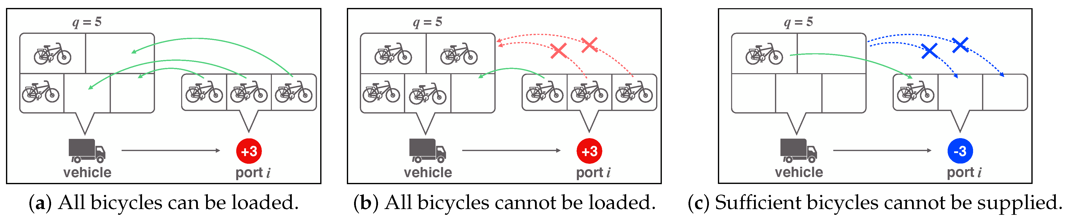
Figure 1 shows examples of the violation of the loading and supplying bicycles. In Figure 1, the capacity of the vehicle is five. In Figure 1a,b, the vehicle must load three bicycles at port i (colored in red). In Figure 1a, the vehicle can take all bicycles because the number of bicycles loaded onto the vehicle before visiting port i is two. On the other hand, in Figure 1b, the number of bicycles loaded onto the vehicle is four. Then, the vehicle can load only one bicycle. Therefore, the two bicycles cannot be loaded onto the vehicle. The number of unloaded bicycles is two, and the loading penalty is added to the objective function, namely $p_{b+}=2$. Figure 1c shows an example of the supplying violation. In Figure 1c, the vehicle must supply three bicycles to port i (colored in blue). However, the number of bicycles loaded onto the vehicle is only one. Therefore, the two bicycles cannot be supplied at port i. The number of unsupplied bicycles is two, and the supplying penalty is added to the objective function, namely $p_{b-}=2$. When $p_{\mathrm{T}}$, $p_{b+}$ and $p_{b-}$ are zero, the solution is a feasible mBSSRP solution. However, if one of them is positive, the solution is an infeasible mBSSRP solution.

In Equation (18), $\alpha$ and $\beta$ are the weight parameters of the penalty. If the parameters are set to a large value, a small constraint violation becomes a large penalty. Nonetheless, it is possible to search for a solution that sufficiently satisfies the mBSSRP constraints. In the actual relocation operation, it may not be possible to obtain a solution that satisfies all of the constraints, i.e., we may not be able to find a feasible mBSSRP solution. In such a case, adjusting the values of $\alpha$ and $\beta$, we can decide on a priority order for the constraints.

3. Heuristic Methods

An optimal solution can be obtained by using an exact algorithm using the mBSSRP formulation and a general-purpose MIP solver. However, for an instance with a large number of ports, it is almost impossible to obtain an optimal solution in a reasonable time frame using the exact algorithm. Therefore, we used an approximation algorithm, a construction method, local search methods and the tabu search as a meta-heuristics method. The construction method is used to construct an initial solution. The local search methods ensure decent downhill dynamics. The tabu search is used to escape from local minima.

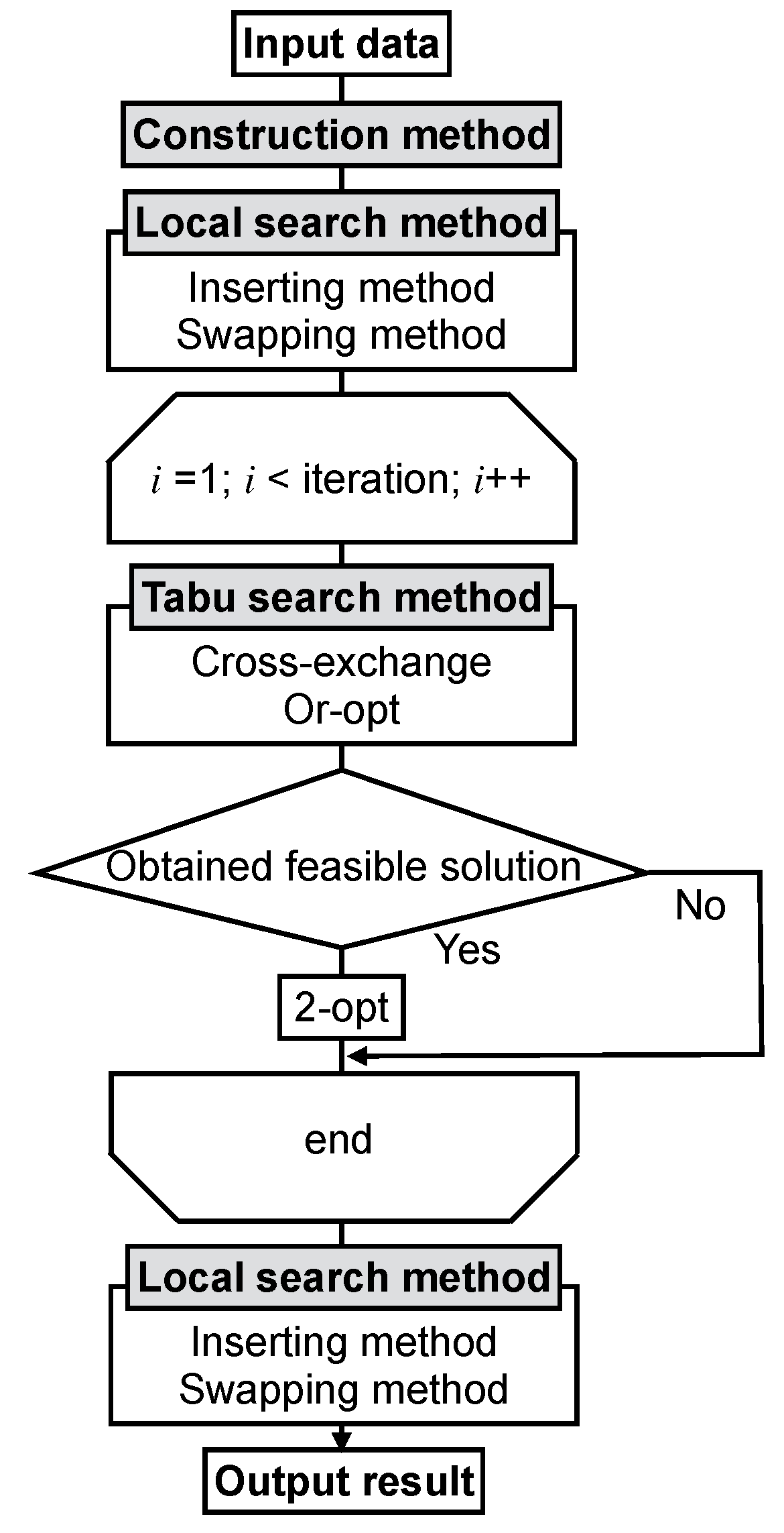
The proposed method can find a solution to mBSSRP or mBSSRP-S in three steps. First, an initial tour is constructed by the construction method. Second, the initial solution is improved by the local search methods, consisting of the inserting method and the swapping method. Then, to find a good solution for mBSSRP, the execution of the CROSS-exchange and the Or-opt are controlled by the tabu search. Figure 2 is a flowchart of the proposed method. In the following subsections, we explain the construction methods, the local search methods and the tabu search in more detail.

3.1. Construction Method

We introduce two construction methods. The first method constructs a feasible solution for the mBSSRP and the second constructs a feasible solution for the mBSSRP-S. The first construction method sequentially inserts a port into a current tour until all ports are visited by a vehicle. We refer to the first construction method as “the cheapest insertion method”. When a port is inserted into the current tour, the resulting new tour must satisfy the constraints of the mBSSRP. The algorithm of the first construction method is described as follows:

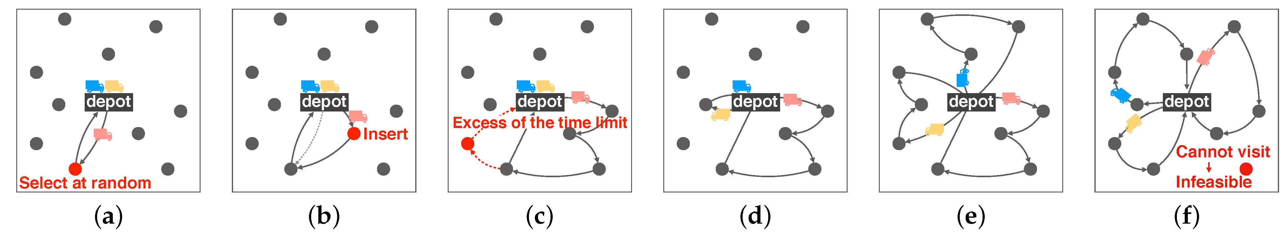
• Port i is randomly selected. If the number of bicycles at port i is negative ($b_i<0$), the vehicle departs from the depot after loading $b_i$ bicycles, supplies $b_i$ bicycles to port i and returns to the depot. However, if $b_i>0$, the empty vehicle goes to port i to load $b_i$ bicycles and returns to the depot. In Figure 3a, the red port is a randomly selected port, and the pink vehicle goes to the selected red port and returns to the depot.
• An unvisited port k is inserted into the current tour. To insert the unvisited port into an edge $(i,j)$ in the current tour, the cost ${\Delta }_{ikj}=t_{ik}+t_{kj}-t_{ij}$ is calculated for all unvisited ports k. If the sub-tour after inserting port k into the edge $(i,j)$ cannot satisfy the constraints of the mBSSRP, this inserting operation is prohibited.
• Port k, where the cost ${\Delta }_{ikj}$ is minimum, is inserted into edge $(i,j)$. In Figure 3b, the red port is inserted into the tour of the pink vehicle.
• When no ports satisfy the constraints, another vehicle goes to the unvisited port nearest to the depot. Figure 3c shows such a case; the red port is inserted into the tour of the pink vehicle; however, the time limit constraint is not satisfied. Therefore, a new vehicle (yellow) goes to the unvisited port nearest to the depot and returns to the depot as shown in Figure 3d.
• Steps 2 to 4 are repeated until all ports are visited once by one of the vehicles (Figure 3e).
• If all vehicles are already used and there exist unvisited ports, the method cannot construct a feasible mBSSRP solution. In Figure 3f, the red port cannot be visited by any vehicle. This is an infeasible solution.

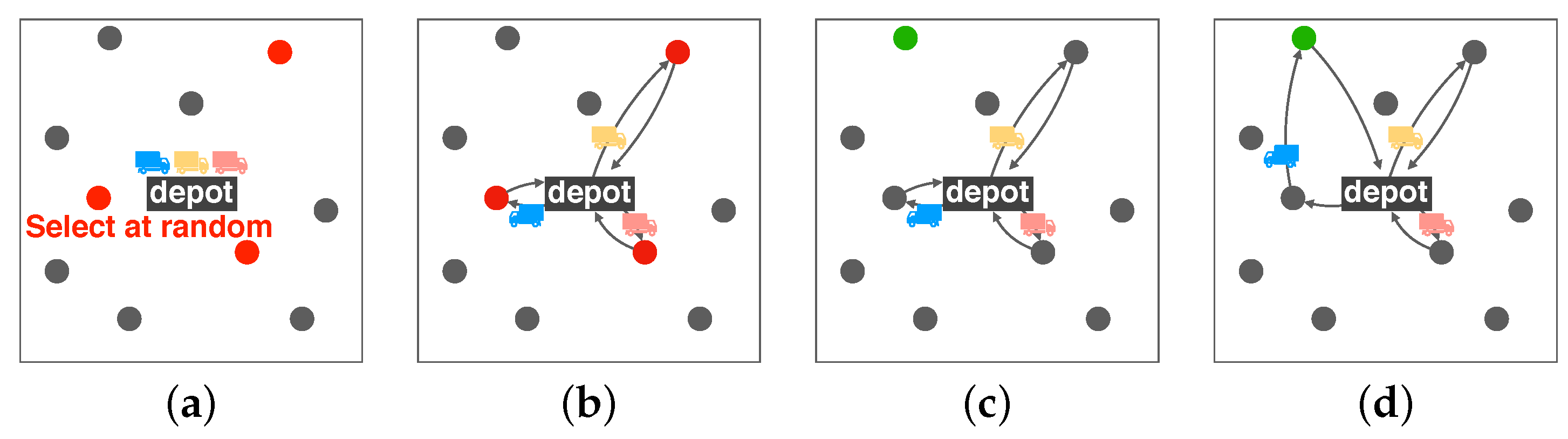
The second construction method is used for the construction of a feasible mBSSRP-S solution. We refer to this as “the farthest insertion method”. It is often used as one of the construction methods for solving the traveling salesman problem. The algorithm of the second construction method is described as follows:

• We randomly select m ports, where m is the number of vehicles. In Figure 4, the number of vehicles is three. Each vehicle goes to one of the selected ports and returns to the depot. In Figure 4a, three red ports are randomly selected. In Figure 4b, the blue, yellow and pink vehicles go to one of the selected ports and return to the depot.
• An unvisited port k, which is the farthest from the depot, is selected. In Figure 4c, the farthest port from the depot is shown in green.
• Port k is inserted between port i and port j in the tour, where ${\Delta }_{ikj}=t_{ik}+t_{kj}-t_{ij}$ is minimized, which means that an increase in the tour length after the insertion of the farthest port is minimum. In Figure 4d, the farthest port (green) is inserted into the tour of the blue vehicle.
• Steps 2 and 3 are repeated until all ports are visited once by one of the vehicles.

3.2. Local Search Methods

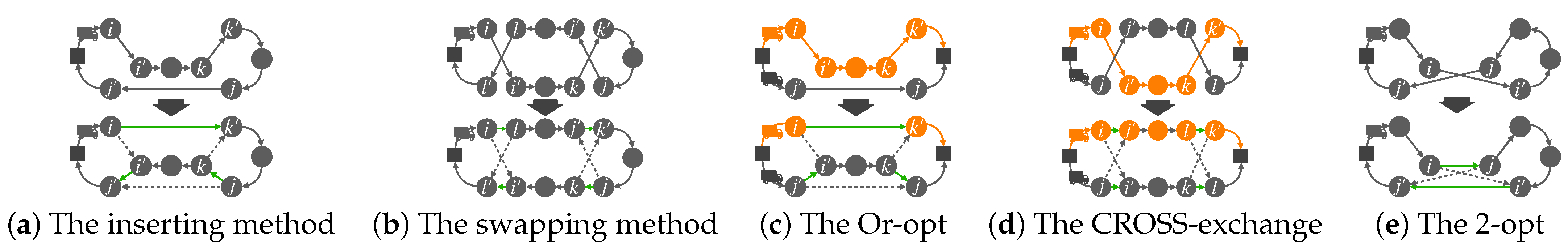
To improve the initial tour, the following five local search methods were used: the inserting method, the swapping method, the Or-opt [29], the CROSS-exchange [30] and the 2-opt method. While the inserting, the swapping and the 2-opt methods improved a single tour, the CROSS-exchange and the Or-opt improved the total travel time using two different tours.

In the inserting method, a partial tour whose length covers a maximum of three ports in a tour is inserted into an edge in the same tour. In Figure 5a, a partial tour $i^{\prime }-k$ is inserted into an edge $(j,j^{\prime })$ in the same tour. The swapping method swaps a partial tour for another partial tour in the same tour. In Figure 5b, a partial tour $i^{\prime }-k$ is swapped for a partial tour $j^{\prime }-l$. The Or-opt inserts a partial tour of a tour into an edge in another tour. In Figure 5c, a partial tour $i^{\prime }-k$ in the orange tour is inserted into an edge $(j,j^{\prime })$ in the gray tour. In the Or-opt, the number of vehicles can be reduced, because of the insertion of ports. The CROSS-exchange replaces a partial tour in a tour with a partial tour in another tour. In Figure 5d, a partial tour $i^{\prime }-k$ in the orange tour is exchanged with a partial tour $j^{\prime }-l$ in the gray tour. The neighborhood solutions of the CROSS-exchange include that of the Or-opt. The 2-opt method deletes two edges in a tour and adds two new edges in the tour. In Figure 5e, two edges $i-i^{\prime }$ and $j-j^{\prime }$ are deleted, and two new edges $i-j$ and $i^{\prime }-j^{\prime }$ are added. The 2-opt method is used to improve a current solution if the current solution is a feasible solution obtained during the searching process using the tabu search.

3.3. Tabu Search Method

Most solutions obtained by the local search methods are locally optimal solutions but not the globally optimal solution. Hence, to find the globally optimal or near-optimal solutions, we used the tabu search [24,25,26]. The tabu search is one of the most powerful meta-heuristic strategies for solving combinatorial optimization problems. In the tabu search, to prevent a periodic search, previous solutions are stored in a tabu list for a certain amount of time. This duration is called a tabu tenure. During the tabu tenure, solutions are prohibited from moving to solutions in the tabu list.

In the proposed method, a current solution moves to the best neighborhood solution generated by the CROSS-exchange or the Or-opt. The combination of ports $i^{\prime }$ and $j^{\prime }$ (Figure 5c,d) is then stored in the tabu list. During the tabu tenure, the CROSS-exchange or the Or-opt cannot be performed on ports $i^{\prime }$ and $j^{\prime }$ because they are now in the tabu list. If a feasible mBSSRP solution is obtained using the tabu search method, the 2-opt algorithm is applied to the feasible solution to obtain a solution that is even better than the current one (Figure 5e). The tabu search explores the solution space of the mBSSRP through many iterations. Finally, the best solution obtained through the tabu search is further improved upon by using the inserting and the swapping methods (Figure 5a,b).

3.4. Dynamically Changing Weight of Penalties

When the penalty values in the mBSSRP-S objective function are zero, the solution is a feasible mBSSRP solution. In contrast, if one of the penalty values is larger than zero, the solution is an infeasible mBSSRP solution. To obtain feasible mBSSRP solutions from mBSSRP-S solutions, the parameters $\alpha$ and $\beta$ in the mBSSRP-S objective function must be set to appropriate values. If the parameters are small, the penalty becomes weak even when the solution has several constraint violations. Then, the method tends to search the infeasible solution space of mBSSRP. Thus, it is difficult to obtain a feasible mBSSRP solution. If the parameters $\alpha$ and $\beta$ are large, the current solution moves to a solution space that has small constraint violations, because these slight constraint violations result in a strong penalty. To perform an effective solution search for a good mBSSRP solution, the values of the parameters $\alpha$ and $\beta$ must be adjusted in accordance with the solution states.

To adjust these values, we introduced a strategy based on a method for solving the vehicle routing problem with time window (VRPTW) [31]. The objective of the VRPTW is to find the shortest tour that serves all customers while satisfying the capacity, time limit and time window constraints associated with each customer. It is difficult to find a feasible solution for the VRPTW due to multiple constraints. To relax the constraints of the VRPTW, the vehicle routing problem with soft time windows (VRPSTW) was proposed. In the VRPSTW, the time windows can be violated if a penalty is paid. To find feasible VRPTW solutions, the weight penalty for the time windows is dynamically changed to obtain many feasible VRPTW solutions [31].

Thus, for the mBSSRP-S study, we extended this method [31] to dynamically adjust the weights of the penalties. In VRPSTW [31], there is a single weight parameter, while in mBSSRP-S, there are two weight parameters $\alpha$ and $\beta$. Thus, we had to consider how to change the values of two parameters. To adjust the weights of the penalties dynamically, the objective function of the mBSSRP-S was modified as follows:

$$z\left(t\right)=\sum _{i\in V}\sum _{j\in V}\sum _{k\in K}{t}_{ij}{x}_{ijk}+\alpha \left(t\right)p_{\mathrm{T}}\left(t\right)+\beta \left(t\right)(p_{\mathrm{q}+}\left(t\right)+p_{\mathrm{q}-}\left(t\right)),$$

(19)

where $z\left(t\right)$ is the objective function of the mBSSRP-S at time t; $\alpha \left(t\right)$ and $\beta \left(t\right)$ are the weights of the penalties for the time limit constraint and the loading and supplying constraints, respectively; $p_{\mathrm{T}}\left(t\right)$ is the excess work time at time t, which extends beyond the time limit T; $p_{\mathrm{q}+}\left(t\right)$ refers to the loading violation of the bicycles at time t, where loading violation is defined as the total number of bicycles exceeding the loading capacity of the vehicle; $p_{\mathrm{q}-}\left(t\right)$ refers to the supplying violation, representing the total number of bicycles that could not be supplied.

In this method, if a feasible solution is obtained at time t, the weight parameter is decreased, making it is easy to move to an infeasible solution at time $t+1$. However, if an infeasible solution is obtained at time t, the weight parameter is increased, making it easy to move to the solution with small constraint violations at time $t+1$. In this study, we propose two methods for adjusting the weights of the penalties.

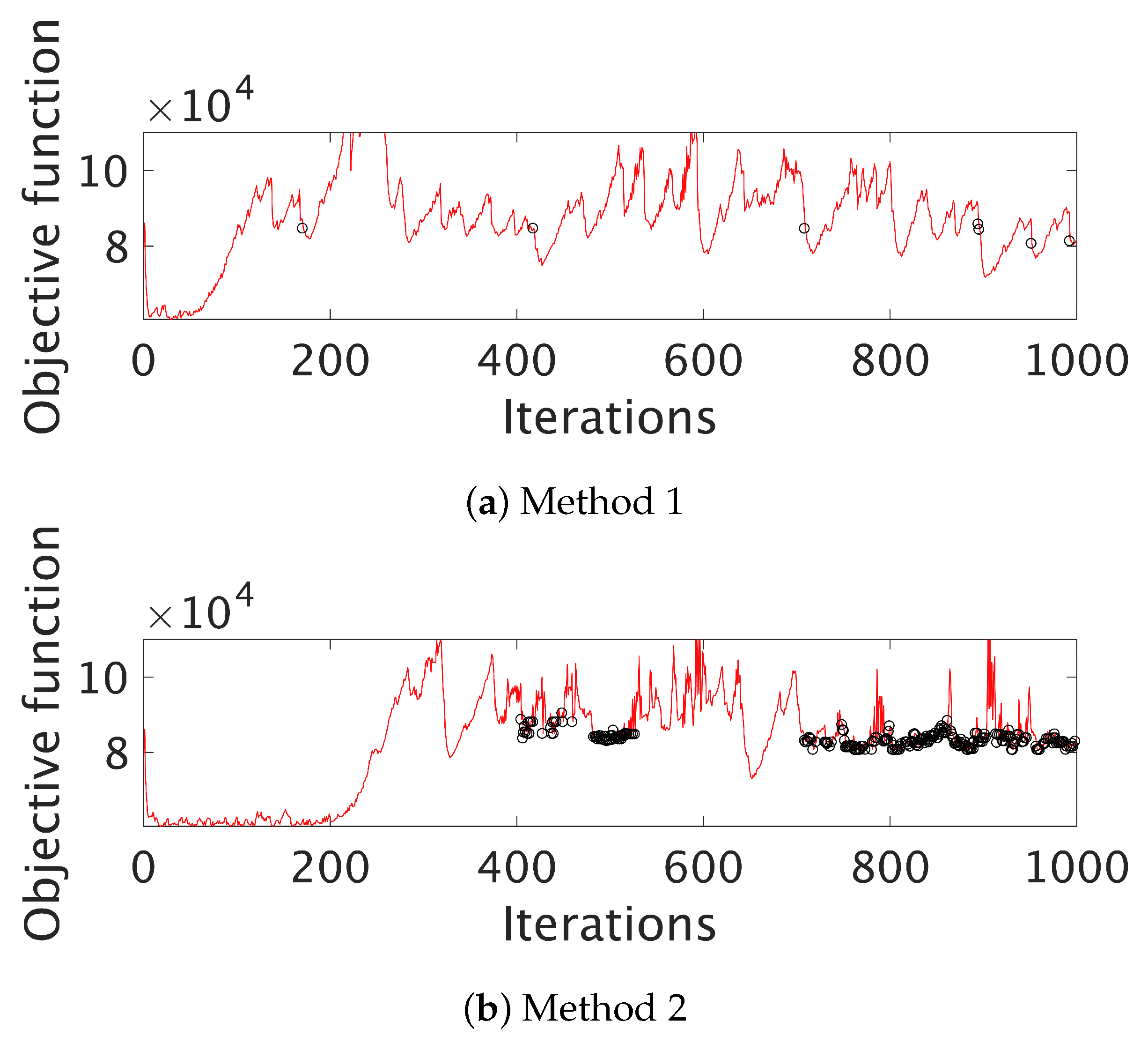
The first method (Method 1) updates the weights through the following equations:

$$\begin{array}{ccc}\hfill \alpha (t+1)& =& \left\{\begin{array}{cc}\lambda \alpha \left(t\right),\hfill & \mathrm{if}{p}_{\mathrm{T}}\left(t\right)>0,\hfill \\ \mu \alpha \left(t\right),\hfill & \mathrm{if}{p}_{\mathrm{T}}\left(t\right)=0,\hfill \end{array}\right.\hfill \end{array}$$

(20)

and

$$\begin{array}{ccc}\hfill \beta (t+1)& =& \left\{\begin{array}{cc}\lambda \beta \left(t\right),\hfill & \mathrm{if}{p}_{\mathrm{q}+}\left(t\right)+p_{\mathrm{q}-}\left(t\right)>0,\hfill \\ \mu \beta \left(t\right),\hfill & \mathrm{if}{p}_{\mathrm{q}+}\left(t\right)+p_{\mathrm{q}-}\left(t\right)=0,\hfill \end{array}\right.\hfill \end{array}$$

(21)

where the parameter $\lambda$ is an increasing parameter ($\lambda >1$) and the $\mu$ is a decreasing parameter ($0<\mu <1$). If the penalty of a solution at time t is positive, the value of the weight corresponding to the penalty is increased. In contrast, if a penalty value is zero, the corresponding weight is decreased. After updating the weights, if the values of the weights are less than 1.0, the weights are set to unity ($\alpha (t+1)=1$ or $\beta (t+1)=1$).

If the solution violates both penalties, Method 1 increases the weights of both constraints to find a solution with a lower penalty at the time of the next iteration. As the weight increases, the searching strategy becomes almost identical to the search used for the feasible mBSSRP solution space.

To search the infeasible mBSSRP solution space widely, we introduced a second method (Method 2). In Method 2, when the solution violates both constraints, first, the values of penalty for the time limit and the loading and supplying constraint are compared. If the penalty of the time limit constraint is larger than that of the loading and supplying constraint, only the weight of the time limit penalty $\alpha \left(t\right)$ is increased. Although the solution violates the loading and supplying constraint, $\beta \left(t\right)$ is decreased. Meanwhile, if the penalty of the loading and supplying constraint is larger, $\beta \left(t\right)$ is increased and $\alpha \left(t\right)$ is decreased. In a combinatorial optimization problem, good solutions have similar structures. Hence, there may be other feasible shorter mBSSRP tours around the feasible mBSSRP solution. In Method 2, if $p_{\mathrm{T}}\left(t\right)=0$ or $p_{\mathrm{b}+}\left(t\right)+p_{\mathrm{b}-}\left(t\right)=0$, the corresponding $\alpha \left(t\right)$ or $\beta \left(t\right)$ is not updated.

Method 2 updates the weights as follows:

$$\begin{array}{ccc}\hfill \alpha (t+1)& =& \left\{\begin{array}{cc}\lambda \alpha \left(t\right)\hfill & \mathrm{if}\alpha \left(t\right)p_{\mathrm{T}}\left(t\right)>\beta \left(t\right)(p_{\mathrm{q}+}\left(t\right)+p_{\mathrm{q}-}\left(t\right)),\mathrm{and}{p}_{\mathrm{T}}\left(t\right)\ne 0,\hfill \\ \mu \alpha \left(t\right)\hfill & \mathrm{if}\alpha \left(t\right)p_{\mathrm{T}}\left(t\right)<\beta \left(t\right)(p_{\mathrm{q}+}\left(t\right)+p_{\mathrm{q}-}\left(t\right)),\mathrm{and}{p}_{\mathrm{T}}\left(t\right)\ne 0,\hfill \\ \alpha \left(t\right)\hfill & \mathrm{if}\alpha \left(t\right)p_{\mathrm{T}}\left(t\right)=\beta \left(t\right)(p_{\mathrm{q}+}\left(t\right)+p_{\mathrm{q}-}\left(t\right)),\mathrm{and}{p}_{\mathrm{T}}\left(t\right)\ne 0,\hfill \\ \alpha \left(t\right)\hfill & \mathrm{if}{p}_{\mathrm{T}}\left(t\right)=0,\hfill \end{array}\right.\hfill \end{array}$$

(22)

and

$$\begin{array}{ccc}\hfill \beta (t+1)& =& \left\{\begin{array}{cc}\lambda \beta \left(t\right)\hfill & \mathrm{if}\alpha \left(t\right)p_{\mathrm{T}}\left(t\right)<\beta \left(t\right)(p_{\mathrm{q}+}\left(t\right)+p_{\mathrm{q}-}\left(t\right)),\mathrm{and}{p}_{\mathrm{q}+}\left(t\right)+p_{\mathrm{q}-}\left(t\right)\ne 0,\hfill \\ \mu \beta \left(t\right)\hfill & \mathrm{if}\alpha \left(t\right)p_{\mathrm{T}}\left(t\right)>\beta \left(t\right)(p_{\mathrm{q}+}\left(t\right)+p_{\mathrm{q}-}\left(t\right)),\mathrm{and}{p}_{\mathrm{q}+}\left(t\right)+p_{\mathrm{q}-}\left(t\right)\ne 0,\hfill \\ \beta \left(t\right)\hfill & \mathrm{if}\alpha \left(t\right)p_{\mathrm{T}}\left(t\right)=\beta \left(t\right)(p_{\mathrm{q}+}\left(t\right)+p_{\mathrm{q}-}\left(t\right)),\mathrm{and}{p}_{\mathrm{q}+}\left(t\right)+p_{\mathrm{q}-}\left(t\right)\ne 0,\hfill \\ \beta \left(t\right)\hfill & \mathrm{if}{p}_{\mathrm{q}+}\left(t\right)+p_{\mathrm{q}-}\left(t\right)=0.\hfill \end{array}\right.\hfill \end{array}$$

(23)

Thus, if both the time limit and the loading and supplying constraints are violated, in Method 1, both parameters $\alpha \left(t\right)$ and $\beta \left(t\right)$ are increased. In Method 2, the parameters $\alpha \left(t\right)$ and $\beta \left(t\right)$ are adjusted after comparing the time limit penalty with the loading and supplying constraint penalty. If the penalties associated with the time limit and the loading and supplying constraints equal 0, both parameters $\alpha \left(t\right)$ and $\beta \left(t\right)$ are decreased in Method 1; however, the parameters $\alpha \left(t\right)$ and $\beta \left(t\right)$ are not updated in Method 2. After updating the weights, if the values of the weights are less than unity, then they are set to unity ($\alpha (t+1)=1$ or $\beta (t+1)=1$).

4. Numerical Experiments

To evaluate the performance of the proposed method, we built a benchmark problem for the mBSSRP. We distributed $n=10,30,50$ ports uniformly in a 10 ${\mathrm{km}}^2$ region. The number of bicycles at port i, $b_i$ was set to a random number integer between $-5$ and $+5$ at intervals of 1. Note that ${\Sigma }_{i=1}^n{b}_i=0$. The number of vehicles was set to a maximum of three. In applying the CROSS-exchange and the Or-opt, if the constraints are satisfied and the number of tours can be decreased, the number of vehicles is decreased such that the relocation of bicycles is performed by one or two vehicles. The capacity of the vehicle was $q=5$. The moving speed of the vehicle was 30 [km/h]. The loading or unloading time of a bicycle was $\tau =2$ [min]. The time limit T was 120 [min] for $n=10$ and 30 and 210 [min] for $n=50$.

4.1. Results of the MIP Solver

First, we performed numerical experiments to find an optimal solution using the mBSSRP formulation and the MIP solver. For the simulation, we used the Gurobi optimizer 9.1.1 [17]. These numerical experiments were performed on an iMac with a 3.2-GHz 4-Core Intel Core i5 processor and 40 GB RAM. If an optimal solution was not obtained within 12 h, then the best solution obtained within that period was output.

Table 3. Optimal or near-optimal solution obtained by the Gurobi optimizer. Symbol “-” means that no feasible solutions can be found by the Gurobi optimizer 9.1.1 within 12 h. Symbol “*” means that an optimal solution can be obtained using the Gurobi optimizer 9.1.1 within 12 h. (a) $n=10$. (b) $n=30$. (c) $n=50$.

(a)
No.	Objective Function	CPU-Time [s]
1	45,346 *	1.31
2	32,530 *	0.21
3	63,209 *	1.37
4	27,522 *	0.43
5	45,971 *	1.20
6	32,828 *	1.44
7	38,623 *	1.82
8	40,304 *	1.20
9	41,640 *	0.76
10	31,825 *	0.93
(b)
No.	Objective Function	CPU-Time [s]
1	80,740 *	307.61
2	78,903 *	43,200.00
3	-	-
4	73,681 *	1048.03
5	72,912 *	21,800.49
6	-	-
7	74,625 *	3499.36
8	68,347 *	1068.09
9	73,328 *	1347.61
10	66,403 *	219.87
(c)
No.	Objective Function	CPU-Time [s]
1	101,119	43,200.00
2	100,356	43,200.00
3	82,201	43,200.00
4	95,257	43,200.00
5	96,297	43,200.00
6	107,727	43,200.00
7	93,003	43,200.00
8	93,003	43,200.00
9	84,409	43,200.00
10	88,029	43,200.00

presents the results of the numerical experiments. The first column contains the instance numbers, the second column provides the values of the objective function, and the third column provides the calculation times. If the CPU time was less than 43,200 [s] (=12 [h]), then an optimal solution was obtained by the Gurobi optimizer. According to Table 3a, for small-sized instances, the optimal solution was obtained for all instances in a short time. However, when the number of ports was increased to 30 or 50, the calculation times became prohibitively long. For instances 3 and 6 of $n=30$ (Table 3b), no feasible solutions were obtained. For instance 2 of $n=30$ (Table 3b) and all instances of $n=50$ (Table 3c), no optimal solutions were found within 12 h. In such cases, the tables display the best solution obtained within the 12 h period.

4.2. Results of the Proposed Method

To evaluate the performance of the proposed method, we generated 50 initial solutions using the cheapest insertion method for the mBSSRP and the farthest insertion method for the mBSSRP-S. The tabu tenure was set to 20, and the number of iterations was set to 1000. The initial weights were set to $\alpha \left(0\right)=1$ and $\beta \left(0\right)=1$. The increasing $\lambda$ and decreasing parameters $\mu$ were set to $1.05$ and $0.7$, respectively. In evaluating the solutions generated by our method, we used the gap between our solution and the optimal or best solutions (Table 3b,c). The gap is defined by the following equation:

$$\mathrm{Gap}[\%]=\frac{\mathrm{Obtained}\mathrm{best}\mathrm{solution}-\mathrm{Optimal}\mathrm{or}\mathrm{Best}\mathrm{solution}}{\mathrm{Optimal}\mathrm{solution}}\times 100.$$

(24)

Thus, small gaps indicate good performance.

Table 4. Results of exploring feasible solution space for solving the mBSSRP. Ave., Best and Worst represent the average, best and worst gaps calculated using Equation (24). Symbol “-” means that no feasible solutions can be obtained. The feasible solutions of the instances 3 and 6 ($n=30$) cannot be found using the latest version of the Gurobi optimizer 9.1.1. For $n=50$, negative values of the best gaps mean that the method can find better solutions than that found by the Gurobi optimizer 9.1.1 within 12 h. Symbol “*” means that an optimal solution can be obtained using the Gurobi optimizer 9.1.1 within 12 h. (a) $n=30$. (b) $n=50$.

(a)
No.	Ave.	Best	Worst	# of Feasible
1	-	-	-	0
2	-	-	-	0
4	-	-	-	0
5	-	-	-	0
7	-	-	-	0
8	1.90	0.00 *	15.95	32
9	-	-	-	0
10	-	-	-	0
(b)
No.	Ave.	Best	Worst	# of Feasible
1	-	-	-	0
2	-	-	-	0
3	4.59	$-1.76$	10.01	35
4	2.96	1.35	3.76	3
6	3.94	1.88	5.99	2
5	0.16	$-3.92$	3.81	11
7	3.44	$-0.62$	7.13	15
8	-	-	-	0
9	3.23	$-0.63$	5.25	20
10	0.79	$-3.14$	5.87	34

,

Table 5. Results of the method using fixed values of weight parameters for $n=30$. Symbol “-” means that no feasible solutions can be obtained. Feasible solutions of instances 3 and 6 cannot be found by the latest version of the Gurobi optimizer 9.1.1 within 12 h. Symbol “*” means that an optimal solution can be obtained using the Gurobi optimizer 9.1.1 within 12 h. (a) $\alpha =200$, $\beta =2000$. (b) $\alpha =1000$, $\beta =10,000$.

(a)
No.	Ave.	Best	Worst	# of Feasible
1	2.40	0.00 *	5.89	21
2	0.79	0.00 *	4.68	41
4	0.82	0.00 *	2.46	3
5	1.48	0.40 *	4.05	9
7	-	-	-	0
8	1.17	0.00 *	4.41	23
9	-	-	-	0
10	1.16	0.00 *	9.98	40
(b)
No.	Ave.	Best	Worst	# of Feasible
1	2.75	0.00 *	9.77	45
2	0.85	0.17 *	12.86	50
4	0.28	0.00 *	4.63	19
5	1.01	0.40 *	4.02	6
7	4.52	0.40 *	7.10	32
8	0.85	0.00 *	6.12	50
9	0.32	0.00 *	1.51	50
10	0.80	0.00 *	10.83	50

,

Table 6. Results of the method using fixed values of weight parameters for $n=50$. Symbol “-” means that no feasible solutions can be obtained. Negative values of average and best gaps mean that the method can find better solutions than that found by using Gurobi optimizer 9.1.1 within 12 h. (a) $\alpha =200$, $\beta =2000$. (b) $\alpha =1000$, $\beta =10,000$.

(a)
No.	Ave.	Best	Worst	# of Feasible
1	2.41	2.41	2.41	1
2	2.51	$-0.41$	9.21	13
3	4.36	$-0.69$	10.71	7
4	5.53	1.60	9.92	9
5	$-0.57$	$-1.68$	0.66	3
6	$-0.23$	$-0.23$	$-0.23$	1
7	3.58	1.19	6.31	3
8	-	-	-	0
9	3.06	$-0.63$	5.26	17
10	0.50	$-3.14$	5.13	19
(b)
No.	Ave.	Best	Worst	# of Feasible
1	1.27	$-1.61$	5.87	47
2	2.57	$-0.50$	11.92	50
3	3.01	$-2.11$	13.31	49
4	3.59	$-0.33$	11.13	48
5	0.83	$-3.92$	4.80	50
6	3.23	$-0.23$	8.62	50
7	1.81	$-0.69$	8.06	50
9	4.33	$-0.64$	11.24	50
10	1.08	$-3.44$	9.78	50

,

Table 7. Results of gaps in the method that dynamically adjusts weights for $n=30$. Feasible solutions of instances 3 and 6 cannot be obtained by the latest version of the Gurobi optimizer 9.1.1 within 12 h. Symbol “*” means that an optimal solution can be obtained using the Gurobi optimizer 9.1.1 within 12 h. (a) Method 1 (Equations (20) and (21)). (b) Method 2 (Equations (22) and (23)).

(a)
No.	Ave.	Best	Worst	# of Feasible
1	2.03	0.00 *	5.74	48
2	1.08	0.00 *	4.13	48
4	0.43	0.00 *	3.21	50
5	1.75	0.00 *	6.18	35
7	5.19	0.40 *	10.18	41
8	0.38	0.00 *	3.51	50
9	1.22	0.00 *	5.33	50
10	3.44	0.00 *	12.36	50
(b)
No.	Ave.	Best	Worst	# of Feasible
1	0.83	0.00 *	3.56	50
2	0.56	0.00 *	3.53	49
4	0.20	0.00 *	5.07	50
5	1.64	0.00 *	4.47	48
7	3.09	0.00 *	6.68	50
8	0.84	0.00 *	5.95	48
9	0.22	0.00 *	0.67	48
10	1.03	0.00 *	12.33	46

and

Table 8. Results of gaps in the method that adjust weight dynamically for $n=50$. Negative values of average and best gaps mean that the methods can find better solutions than that found using the Gurobi optimizer 9.1.1 within 12 h. (a) Method 1 (Equations (20) and (21)). (b) Method 2 (Equations (22) and (23)).

(a)
No.	Ave.	Best	Worst	# of Feasible
1	0.26	$-1.60$	2.51	50
2	0.57	$-0.41$	3.15	50
3	1.55	$-2.11$	8.49	50
4	0.89	$-0.33$	6.49	50
5	$-0.09$	$-3.30$	3.43	50
6	1.73	$-0.31$	5.94	50
7	0.90	$-0.69$	6.56	50
9	2.02	$-0.10$	4.87	50
10	$-1.32$	$-3.40$	2.19	50
(b)
No.	Ave.	Best	Worst	# of Feasible
1	1.47	$-1.66$	5.47	50
2	2.24	$-0.50$	8.51	49
3	2.99	$-2.11$	11.48	49
4	2.20	$-0.33$	22.49	50
5	0.80	$-3.61$	7.60	50
6	3.60	$-0.69$	9.28	44
7	1.54	$-0.69$	6.89	48
9	3.23	$-0.15$	11.40	50
10	0.59	$-3.39$	10.78	38

present the results. The first column provides the instance numbers and the second to fourth columns present the average gaps obtained after 50 trials of the proposed method with the best and worst gaps as determined from the optimal or best solution. The gaps were calculated using Equation (24). The fifth column states the number of feasible solutions obtained during 50 trials.

As observed in Table 4, the method that only searches the feasible solution space does not yield a feasible mBSSRP solution for $n=30$ and 50. In Table 4a, “-” indicates that the feasible solutions are not obtained. Then, for instances 3, 5, 7, 9 and 10 of $n=50$ (Table 4b), the best gaps take negative values, which means that the method exploring the feasible solution space obtained better solutions than those obtained by the Gurobi optimizer 9.1.1 in 12 h. From Table 4, we cannot obtain feasible solutions for most of the instances. These results indicate that it is difficult to find feasible mBSSRP solutions when only the feasible solution space is explored.

Therefore, to find feasible mBSSRP solutions, we solved the mBSSRP-S with fixed values of the weight parameters. Table 5 and Table 6 present the results. With the Gurobi optimizer, it takes about 12 h for 30 ports, and more than 12 h for 50 ports to obtain feasible solutions. Such long times are not realistic. Meanwhile, the average calculation times of the proposed method are 14.7 [s] ($n=30$) and 56.5 [s] ($n=50$). Therefore, the proposed method can obtain better results, in a time shorter than that required by the Gurobi optimizer.

As observed in Table 4a and Table 5a, the method that explores both feasible and infeasible solution spaces of the mBSSRP obtains many feasible solutions compared to the method that searches only the feasible solution space. In addition, according to Table 5a,b, when the parameters $\alpha$ and $\beta$ have large values, the number of feasible solutions increases, and the average gap indicates that the method performs well. Moreover, the method that explores both the feasible and infeasible solution spaces finds optimal solutions for multiple instances. The difference between the best and worst gaps is large for $n=30$ (Table 3). Table 4b and Table 6 indicate that for $n=50$, we can obtain numerous feasible solutions when the parameters $\alpha$ and $\beta$ have large values.

Table 7 and Table 8 present the results obtained using the method of dynamically adjusted parameters. From Table 7 and Table 8, the number of feasible solutions is 50 for almost all instances. The difference between the best gap and the worst gaps is smaller than that of the fixed case, as can be observed in Table 5 and Table 6. The results indicate that the weight adjusting method can effectively control the search in the feasible and infeasible solution spaces. However, there is no significant difference between Method 1 and Method 2.

The searching processes used in Method 1 and Method 2 when solving mBSSRP-S are shown in Figure 6. The horizontal axis shows the number of iterations and the vertical axis shows the objective function value (Equation (19)). In Figure 6, it is observed that feasible mBSSRP solutions are not obtained (black circle) with 200 iterations in Method 1 and with 400 iterations in Method 2. The parameters $\alpha \left(t\right)$ and $\beta \left(t\right)$ were adjusted using Equations (20) and (21) in Method 1, and Equations (22) and (23) in Method 2. After these phases, as observed in Figure 6a, Method 1 finds several feasible mBSSRP solutions with 1000 iterations. However, Method 2 finds more feasible solutions than Method 1 according to Figure 6b. When the penalty value is zero, Method 2 does not update the penalty weight because the current value is appropriate for conducting a search on feasible mBSSRP solutions. Once feasible mBSSRP solutions are obtained, Method 2 conducts repeated searches for more feasible solutions.

5. Conclusions

In this study, to adjust the number of bicycles at ports in BSS, we solved the mBSSRP. However, it is difficult to obtain feasible mBSSRP solutions because of strict constraints such as the time limit, the capacity and the loading and supplying constraints.

Thus, to find feasible solutions for problems with strict constraints, we developed a strategy of searching not only the feasible solution space but also the infeasible solution space. To explore both the feasible and infeasible mBSSRP solution spaces, we introduced the mBSSRP-S formulation whereby some constraints were removed and penalties were added to the objective function for constraint violation. In addition, we introduced two methods for dynamically adjusting the weights of the penalties, to enhance performance, by effectively searching the feasible and infeasible solution spaces.

The results of the numerical experiments demonstrated that the proposed method could find feasible solutions for almost all benchmark problems while identifying the optimal solutions as well. Thus, it is effective to search both the feasible and infeasible solution spaces. Moreover, we could enhance the performance of our process by introducing a method for dynamically adjusting the weights for solving the mBSSRP-S; namely, we were able to explore the infeasible solution space of the mBSSRP effectively. In this study, we proposed a strategy of searching the feasible and infeasible solutions and showed that the proposed strategy works well for instances of mBSSRP with 30 and 50 ports.

In the future, to obtain an optimal solution for larger instances using the MIP solver, we will propose a more effective formulation with a smaller number of variables and constraints. Although we used flow formulation (FF) to eliminate sub-tours in our study, we also examined Miler, Tucker and Zemlin (MTZ) [32] formulation and conducted numerical experiments. With FF, an optimal solution was obtained in a shorter time, possibly due to the automatic cut generation function of the Gurobi optimizer. Although an important issue, this was not investigated any further as it was not the focus of the current study.

In the numerical experiments, we used original benchmark instances because there are no suitable research examples on BSS restoration. However, generating and sharing benchmark instances in this field as well as comparing the performance of the proposed methods with existing ones are important issues to be addressed in the future. In addition, to find good near-optimal solutions for large-scale instances, we intend to implement algorithms using a meta-strategy, such as simulated annealing, genetic algorithm and ant colony algorithm, and compare the performances. With the current relocation operation, it may not be possible to obtain a solution that satisfies all conditions; namely, we may not be able to find a feasible mBSSRP solution. In such a case, we must prioritize the constraints.

In a real BSS, the number of bicycles and empty docks at each port will change during the relocation operation. Therefore, it is impossible to perfectly restore the BSS to its initial state. An operational goal of the BSS is to always satisfy the user demand: users can rent bicycles at any port and return bicycles to any port, any time during the day. To achieve this goal, we need to predict the travel demands of the users in order to efficiently relocate the bicycles by using the predicted data. To resolve this issue, it will be necessary to analyze the occupancy level [33] and to come up with an efficient prediction model [34], based on actual travel history data that are available for New York [35], Washington D.C. [36] and Boston [37].

In this study, we used scenarios that randomly placed ports and compared the performance of the proposed method, which explores both the feasible and infeasible solution spaces, with the one that explores only the feasible solution space. To apply the proposed strategy to real-world problems, different scenarios have to be entertained. One possible strategy is to use real-life information from the rented and returned bicycle data of actual travel history data [35,36,37]. This information would include the distribution of bicycles at each port as well as the use frequency of the ports. Using this information, more effective strategies can be designed to solve real-world problems. Introducing additional soft constraints could also be beneficial in improving the performance of real-world BSS.

In this study, to adjust and control the parameters $\alpha$ and $\beta$ dynamically, we searched all neighborhood solutions of the CROSS-exchange and the Or-opt. However, a long time is needed to search for all neighborhood solutions of the CROSS-exchange and the Or-opt. When we deal with a larger number of ports or more complex problems with soft constraints, the calculation time further increases. Thus, as a future step, to reduce the calculation time, one of the possible directions is to reduce the number of neighborhood solutions by not searching all neighborhood solutions in the CROSS-exchange and the Or-opt.