
The Study on Internal Flow Characteristics of Disc Filter under Different Working Condition

 ,
,
Abstract
:1. Introduction
2. Materials and Methods
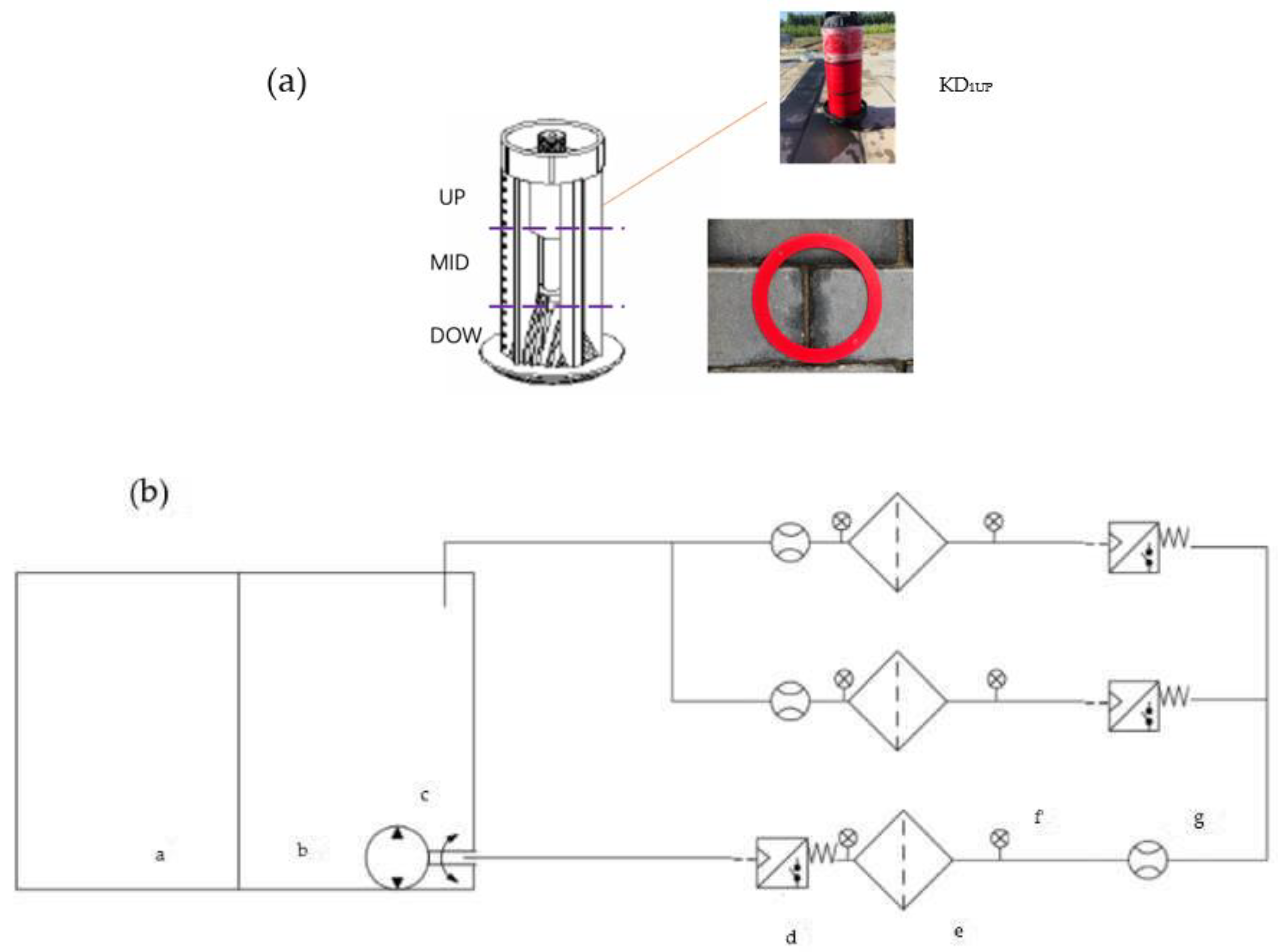
2.1. Working Setup
2.2. Experimental Design
2.3. Model Setting
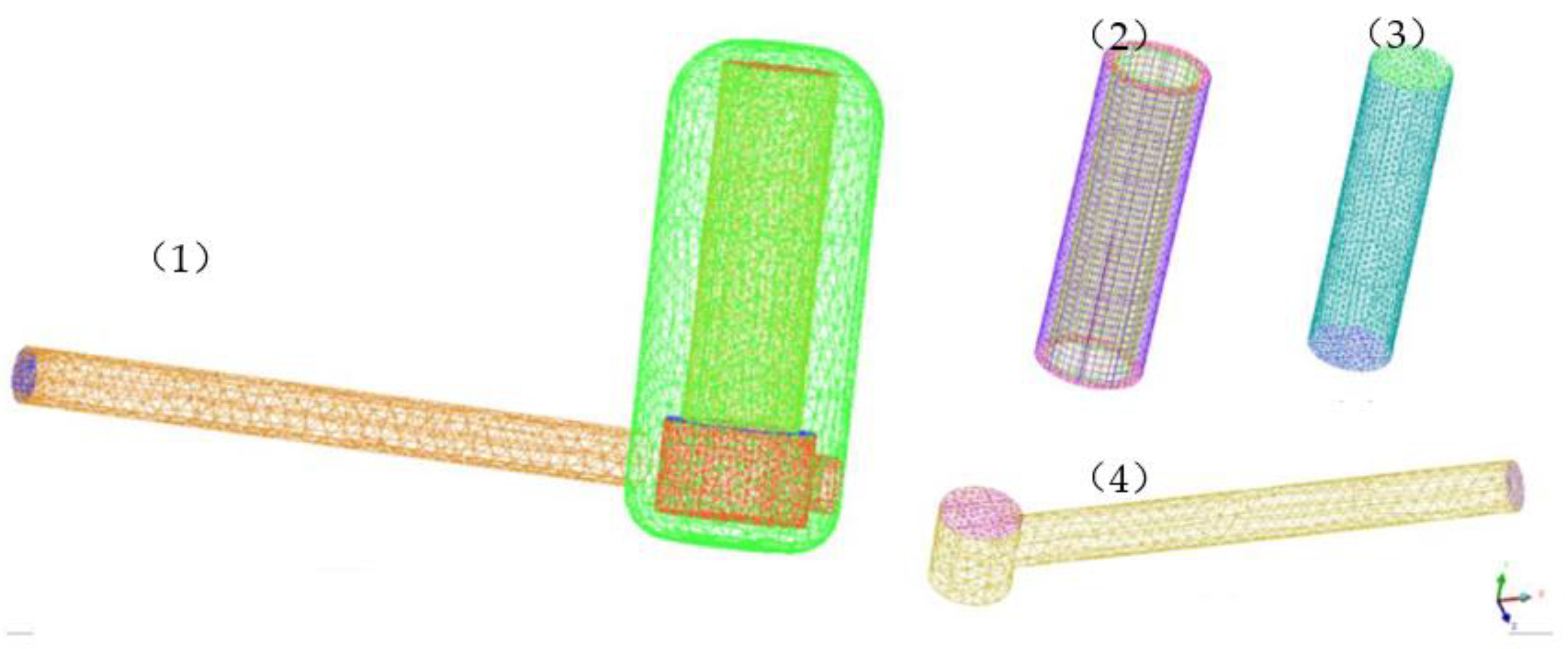
2.4. 3D Model Setting
2.4.1. The Mesh Setup
2.4.2. Calculation Model
2.4.3. Boundary Conditions and Solved Model
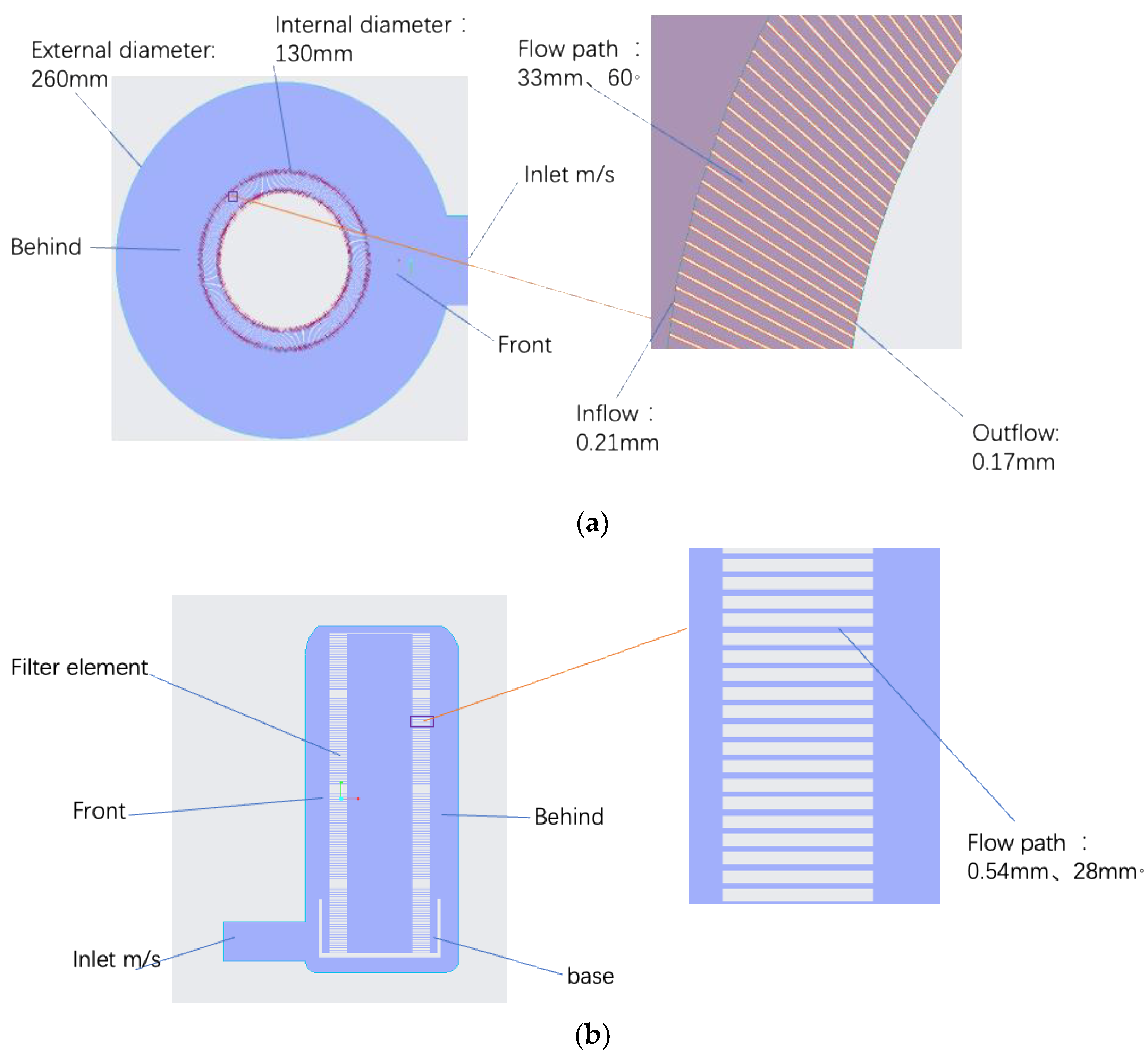
2.5. 2D Model Setting
2.6. Analysis Method
3. Results
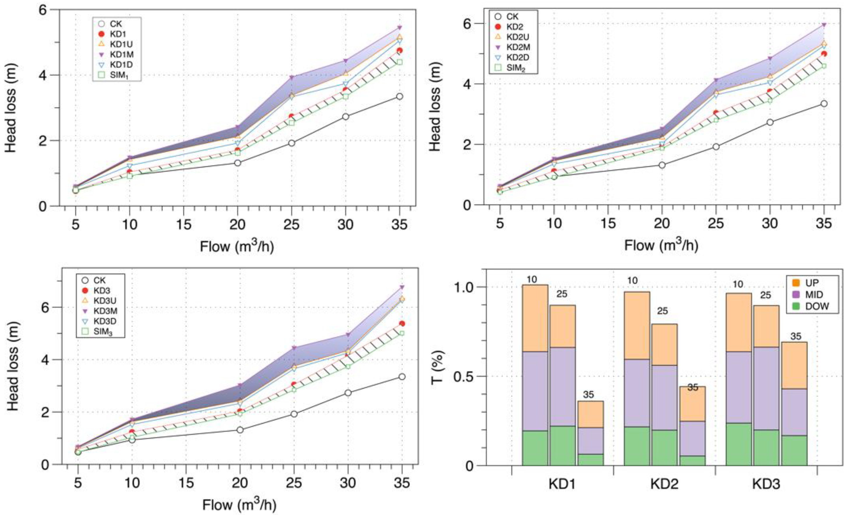
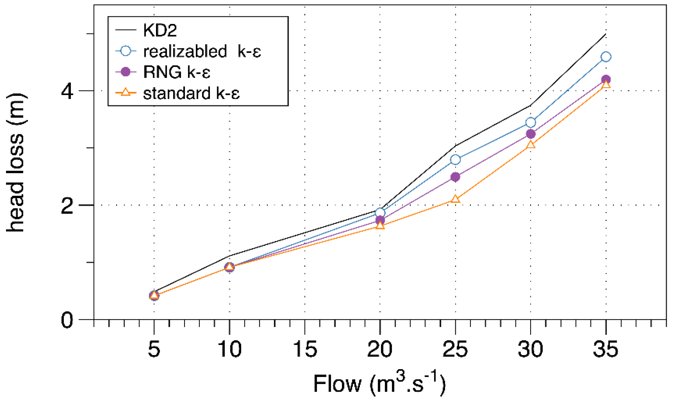
3.1. Filter Test
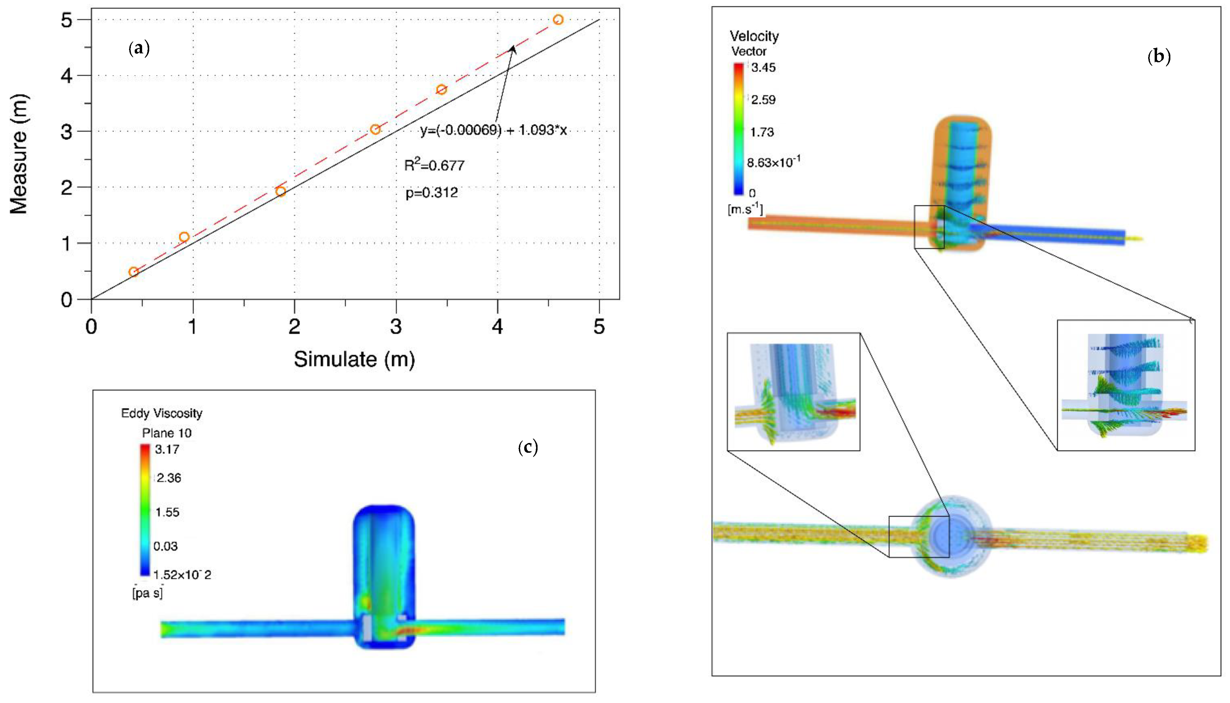
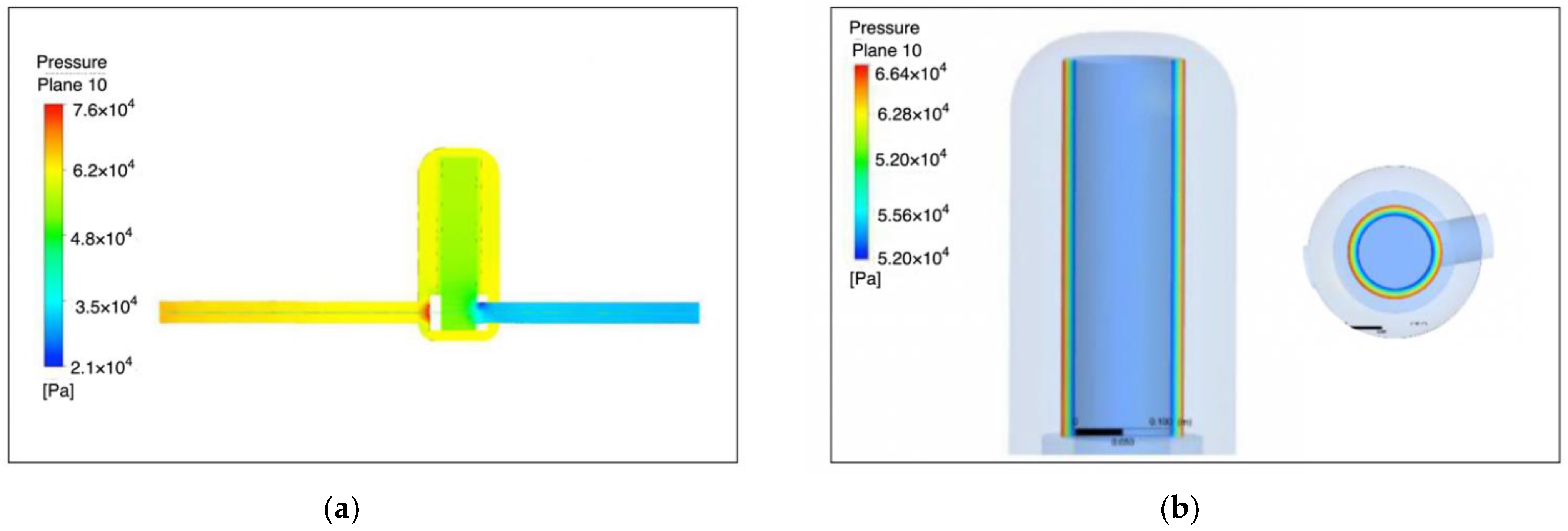
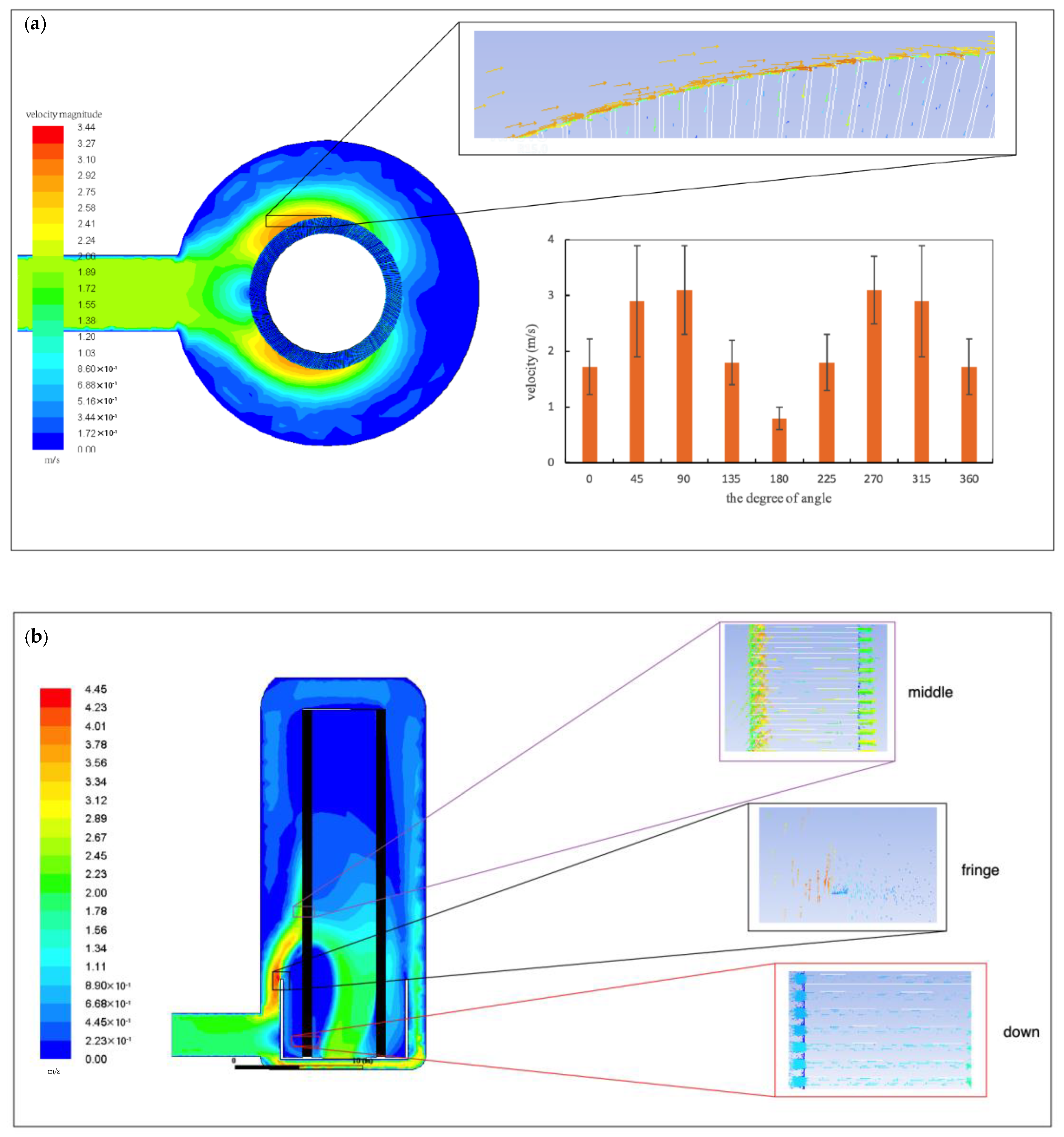
3.2. Macroscopic Simulation
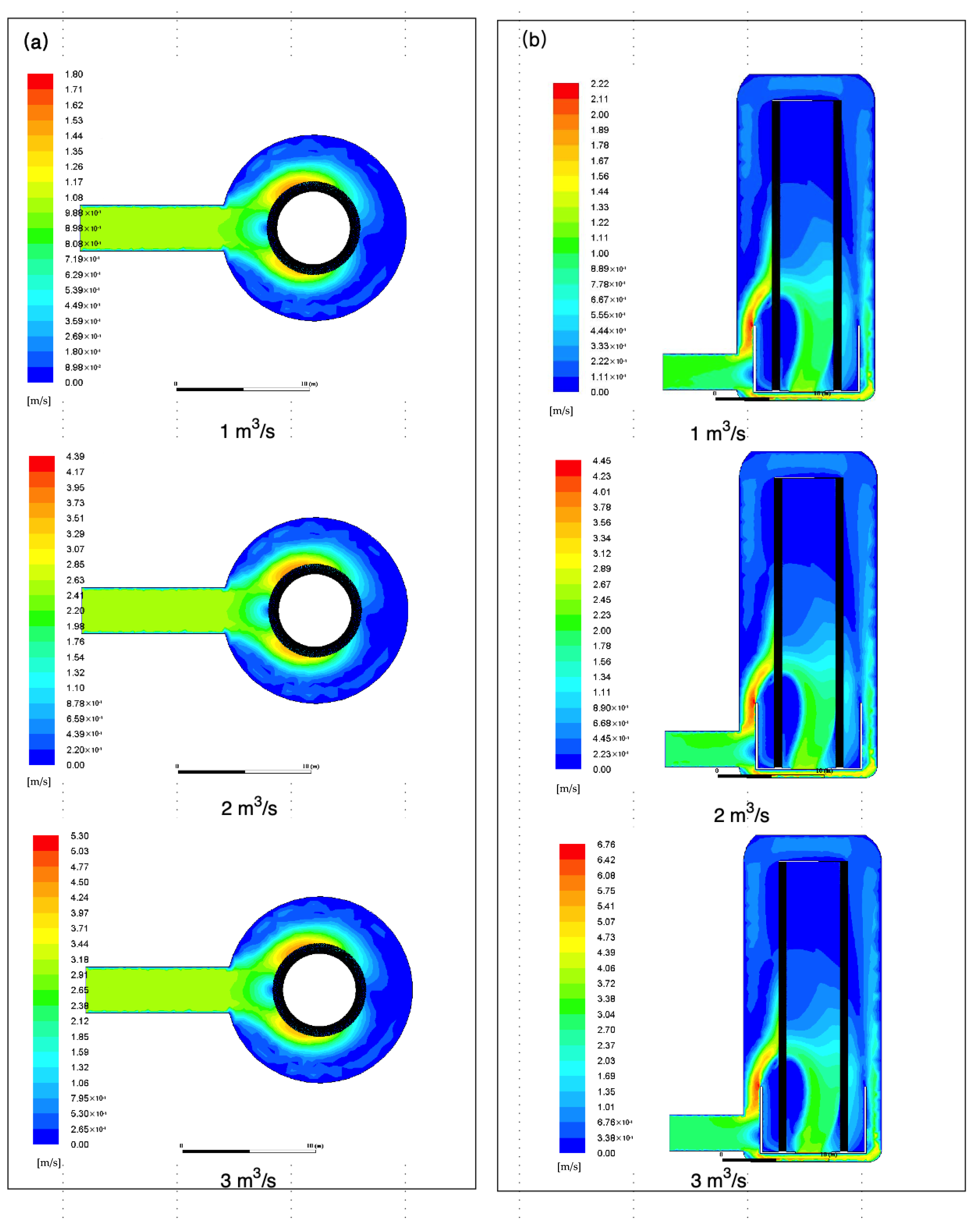
3.3. Horizontal Simple Simulation
3.4. Vertical Simple Simulation
4. Discussion
5. Conclusions
Author Contributions
Funding
Institutional Review Board Statement
Informed Consent Statement
Data Availability Statement
Conflicts of Interest
Appendix A

| Program | Size/mm |
|---|---|
| Diameter of inlet | 63.00 |
| Length of inlet | 750.00 |
| Length of outlet | 510.00 |
| External diameter of filter element | 130.00 |
| Inner diameter of filter element | 102.00 |
| Diameter of DF shell | 240.00 |
| Total high of DF | 520.00 |
| High of filter element | 360.00 |
| High of base | 105.00 |


References
- Puig-Bargués, J.; Barragán, J.; Cartagena, F. Development of Equations for Calculating the Head Loss in Effluent Filtration in Microirrigation Systems Using Dimensional Analysis. Biosyst. Eng. 2005, 92, 383–390. [Google Scholar] [CrossRef]
- Zong, Q.; Zheng, T.; Liu, H.; Li, C. Development of Head Loss Equations for Self-Cleaning Screen Filters in Drip Irrigation Systems Using Dimensional Analysis. Biosyst. Eng. 2015, 133, 116–127. [Google Scholar] [CrossRef]
- Capra, A.; Scicolone, B. Emitter and Filter Tests for Wastewater Reuse by Drip Irrigation. Agric. Water Manag. 2007, 68, 135–149. [Google Scholar] [CrossRef]
- Duran-Ros, M.; Puig-Bargués, J.; Arbat, G.; Barragán, J.; Cartagena, F. Effect of Filter, Emitter and Location on Clogging When Using Effluents. Agric. Water Manag. 2009, 96, 67–79. [Google Scholar] [CrossRef]
- Wu, W.; Wei, C.; Liu, H.; Yin, S.; Zhe, B.; Yong, N. A Dimensional Analysis Model for the Calculation of Head LosscDue to Disc Filters in Drip Irrigation Systems. Irrig. Drain. 2014, 63, 349–358. [Google Scholar] [CrossRef]
- Gyasi-Agyei; Yeboah A Bayesian Approach for Identifying Drip Emitter Insertion Head Loss Coefficients. Biosyst. Eng. 2013, 116, 75–87. [CrossRef]
- Li, Y.; Yang, P.; Xu, T.; Ren, S.; Lin, X.; Wei, R.; Xu, H. CFD and Digital Particle Tracking to Assess Flow Characteristics in the Labyrinth Flow Path of a Drip Irrigation Emitter. Irrig. Sci. 2008, 26, 427–438. [Google Scholar] [CrossRef]
- Feng, J.; Li, Y.; Wang, W.; Xue, S. Effect of Optimization Forms of Flow Path on Emitter Hydraulic and Anti-Clogging Performance in Drip Irrigation System. Irrig. Sci. 2017, 36, 37–47. [Google Scholar] [CrossRef]
- Li, W.Y.; Zhang, X.Y.; Shuai, Z.J.; Jiang, C.X.; Li, F.C. CFD Numerical Simulation of the Complex Turbulent Flow Field in an Axial-Flow Water Pump. Adv. Mech. Eng. 2014, 6, 521706. [Google Scholar] [CrossRef]
- Zhang, J.; Xu, J.; Huang, X.; Li, J.; Han, Q.; Li, H. Research Status and Development Trend of Disc Filter in Micro-Irrigation. Water Sav. Irrig. 2015, 3, 59–65. [Google Scholar]
- Gilbert, R.G.; Nakayama, F.S.; Bucks, D.A.; French, O.F.; Adamson, K.C.; Johnson, R.M. Trickle Irrigation: Predominant Bacteria in Treated Colorado River Water and Biologically Clogged Emitters. Irrig. Sci. 1982, 3, 123–132. [Google Scholar] [CrossRef]
- Hou, J.X.; Zhang, Y.C. Study on Filtration Performance of Rotary Disc Filter with Different Filter Discs. Adv. Mater. Res. 2013, 610–613, 1265–1269. [Google Scholar] [CrossRef]
- Hanly, K.; Grimes, R.; Walsh, E.; Rodgers, B.; Punch, J. The Effect of Reynolds Number on the Aerodynamic Performance of Micro Radial Flow Fans. In Proceedings of the ASME 2005 Summer Heat Transfer Conference Collocated with the ASME 2005 Pacific Rim Technical Conference and Exhibition on Integration and Packaging of MEMS, NEMS, and Electronic Systems, San Francisco, CA, USA, 17–22 July 2005; pp. 549–552. [Google Scholar] [CrossRef]
- Li, H.; Li, H.; Huang, X.Q.; Han, Q.; Zhang, J.; Sun, H.; Li, W. Numerical Simulation and Optimization of Micro Irrigation Disc Filter. J. Irrig. Drain. 2016, 35, 1–5. [Google Scholar] [CrossRef]
- Wang, X.; Gao, S.; Xia, L.; Xu, P. Numerical Simulation and Structural Optimization of Screen Filter in Micro-Irrigation. J. Drain. Irrig. Mach. Eng. 2013, 31, 719–723. [Google Scholar] [CrossRef]
- Yadav, A.S. CFD Investigation of Effect of Relative Roughness Height on Nusselt Number and Friction Factor in an Artificially Roughened Solar Air Heater. J. Chin. Inst. Eng. 2015, 38, 494–502. [Google Scholar] [CrossRef]
- Yadav, A.S.; Sharma, S.K. Numerical Simulation of Ribbed Solar Air Heater. In Advances in Fluid and Thermal Engineering; Select Proceedings of FLAME 2020; Springer: Singapore, 2021; pp. 549–558. [Google Scholar]
- ANSYS Inc. ANSYS Fluent User Guide; ANSYS Inc.: Pittsburgh, PA, USA, 2001. [Google Scholar]


| Nov. | Test Items | Value |
|---|---|---|
| 1 | pH | 7.8 |
| 2 | Total suspended solid (TSS) mg/L | 7.7 |
| 3 | Total hardness mg/L | 983 |
| 4 | Chemical Oxygen Demand (COD) mg/L | 0.74 |
| 5 | Chloride mg/L | 167 |
| Nov | Filter Accuracy | Disc Number | Weight (g) | Rated Pressure (MPa) | Rated Discharge (m3/h) | Groove Number |
|---|---|---|---|---|---|---|
| KD1 | 80 | 229 | 4.02 | 0.1 | 30 | 590 |
| KD2 | 120 | 283 | 4.31 | 0.1 | 30 | 680 |
| KD3 | 150 | 365 | 3.29 | 0.1 | 30 | 710 |
Publisher’s Note: MDPI stays neutral with regard to jurisdictional claims in published maps and institutional affiliations. |
© 2021 by the authors. Licensee MDPI, Basel, Switzerland. This article is an open access article distributed under the terms and conditions of the Creative Commons Attribution (CC BY) license (https://creativecommons.org/licenses/by/4.0/).
Share and Cite
Chi, Y.; Yang, P.; Ma, Z.; Wang, H.; Liu, Y.; Jiang, B.; Hu, Z. The Study on Internal Flow Characteristics of Disc Filter under Different Working Condition. Appl. Sci. 2021, 11, 7715. https://doi.org/10.3390/app11167715
Chi Y, Yang P, Ma Z, Wang H, Liu Y, Jiang B, Hu Z. The Study on Internal Flow Characteristics of Disc Filter under Different Working Condition. Applied Sciences. 2021; 11(16):7715. https://doi.org/10.3390/app11167715
Chicago/Turabian StyleChi, Yanbing, Peiling Yang, Zixuan Ma, Haiying Wang, Yuxuan Liu, Bingbing Jiang, and Zongguang Hu. 2021. "The Study on Internal Flow Characteristics of Disc Filter under Different Working Condition" Applied Sciences 11, no. 16: 7715. https://doi.org/10.3390/app11167715