Lightweight Convolutional Neural Networks with Model-Switching Architecture for Multi-Scenario Road Semantic Segmentation

Abstract

A convolutional neural network (CNN) that was trained using datasets for multiple scenarios was proposed to facilitate real-time road semantic segmentation for various scenarios encountered in autonomous driving. However, the CNN inhibited the mutual suppression effect between weights; thus, it did not perform as well as a network that was trained using a single scenario. To address this limitation, we used a model-switching architecture in the network and maintained the optimal weights of each individual model which required considerable space and computation. We, subsequently, incorporated a lightweight process into the model to reduce the model size and computational load. The experimental results indicated that the proposed lightweight CNN with a model-switching architecture outperformed and was faster than the conventional methods across multiple scenarios in road semantic segmentation.

1. Introduction

Semantic segmentation is an important road detection application for autonomous driving. This application must be both accurate and able to operate in real-time to ensure passenger’s safety. Existing convolutional neural networks (CNNs) are effective for road semantic segmentation. However, variations in road conditions, weather, and the time of the day affect the detection stability and reduce the accuracy of the semantic segmentation.

To achieve a stable and accurate semantic segmentation under diverse road conditions, we propose a convolutional neural network (CNN) with a model-switching architecture (MSA) that was trained using data with variations in terms of road conditions, weather, and time of day. The proposed CNN optimizes multi-model deep learning by using diverse data, and the model-switching architecture enables it to select the most appropriate model for the context detection on the basis of CNN classifiers. Training using multiple models avoids the problem of reduced detection performance due to a mutual suppression between weights, which occurs when a single-model CNN is trained using the data of multiple contexts.

However, semantic segmentation using a multi-model CNN with classifiers for different contexts and model-switching results in a tremendous computation load. There-fore, we additionally propose a lightweight method to facilitate CNN-based semantic segmentation by using CNN classifiers and multiple models to achieve a specific level of performance, reduce the number of calculations, and increase the calculation speed. The article is organized as follows: Section 2 introduces different types of road semantic segmentation. Section 3 presents proposed methods. Section 4 is the experiment results. Section 5 is our conclusion.

The main contributions of this paper are:

• Mutual suppression between weights, which occurs in a single-model CNN, is addressed using a multi-model CNN with model-switching architecture for semantic segmentation given diverse road situations.
• Through the use of lightweight processes in the CNN, the model size and computational load were reduced to increase the execution speed.

2. Related Work

Deep learning has considerable performance in computer vision, especially the convolutional neural network, which is widely used in computer vision. Since 2012, AlexNet [1] had good performance in the ImageNet Image Recognition Challenge in 2012, various convolutional neural networks have been created to achieve better performance, such as the ResNet series [2,3,4] and NASNet series [5,6,7,8]. Additionally, the MobileNet series [9,10,11], ShuffleNet series [12,13], and EfficientNet series [14,15] which have outstanding performance while being lightweight. The field of image recognition is also the first field to use convolutional neural networks.

However, image recognition is not the most accurate method of recognition. In order to further mark the objects to be recognized on the pixels of the image, semantic segmentation was developed. Since FCN [16] performed well in the field of semantic segmentation in 2014, many methods have been created in the field of deep convolutional networks in semantic segmentation. Since SegNet [17] was proposed, which first used an encode–decode structure, the UNet series [18,19,20], which has outstanding performance in medical imaging and recent application in the field of image semantic segmentation, and 3D LiDAR semantic segmentation, transformers [21,22,23] all use the encode–decode structure.

In addition to the encode–decode structure, PSPNet [24], which is known for its pyramid pooling, also has had a profound impact on the development of semantic segmentation. DenseASPP [25], which has atrous convolution, is also a pyramid pooling structure, and the DeepLab series [26,27,28,29] have been inspired by the encode–decode structure and the pyramid pooling structure.

Road semantic segmentation is a crucial part in the field of autonomous driving. There are two main methods for road semantic segmentation. The first method is the pure image-based method [30,31,32,33,34,35,36] which is commonly used. In order to further improve the accuracy, the multi-sensor fusion method [37,38,39,40,41,42] is also a commonly used method for drivable space detection. SNE-RoadSeg+ [43] uses a combination of depth images and RGB images, adding more depth information to improve the detection effect. However, compared with LiDAR, LiDAR has a higher stability and better robustness to solve various situations. Therefore, LiDAR and image fusion methods, such as PLARD+ [44], are also commonly used methods for drivable detection. However, the algorithm of multi-sensor fusion is more complicated. Different sensors, different receiving ranges, different receiving speeds, and the amount of data that the computing unit can process at a time is also different, and the calibration is also more complicated. The equipment is also more expensive, and it needs to be able to process data from different sensors, which also makes an amount of calculations. In order to solve this problem, this paper proposes a simple but effective convolutional neural network named Light-Weight Fast VGG (LWF-VGG) that modified VGG16 [45] to detect the drivable space of autonomous driving vehicle. Additionally, in order to be able to cope with the effect of different time and climate on the road image, this paper proposes a model-switching architecture to solve various road conditions.

3. Proposed Lightweight CNN with an MSA

The proposed CNN is illustrated in Figure 1. It is based on a model-switching architecture that selects a model for semantic segmentation depending on the road conditions. This algorithm reduces misjudgments and increases segmentation accuracy. To allow a faster execution, lightweight processes are incorporated into the network to reduce the computational load. These two features of the proposed neural network are described in the following section.

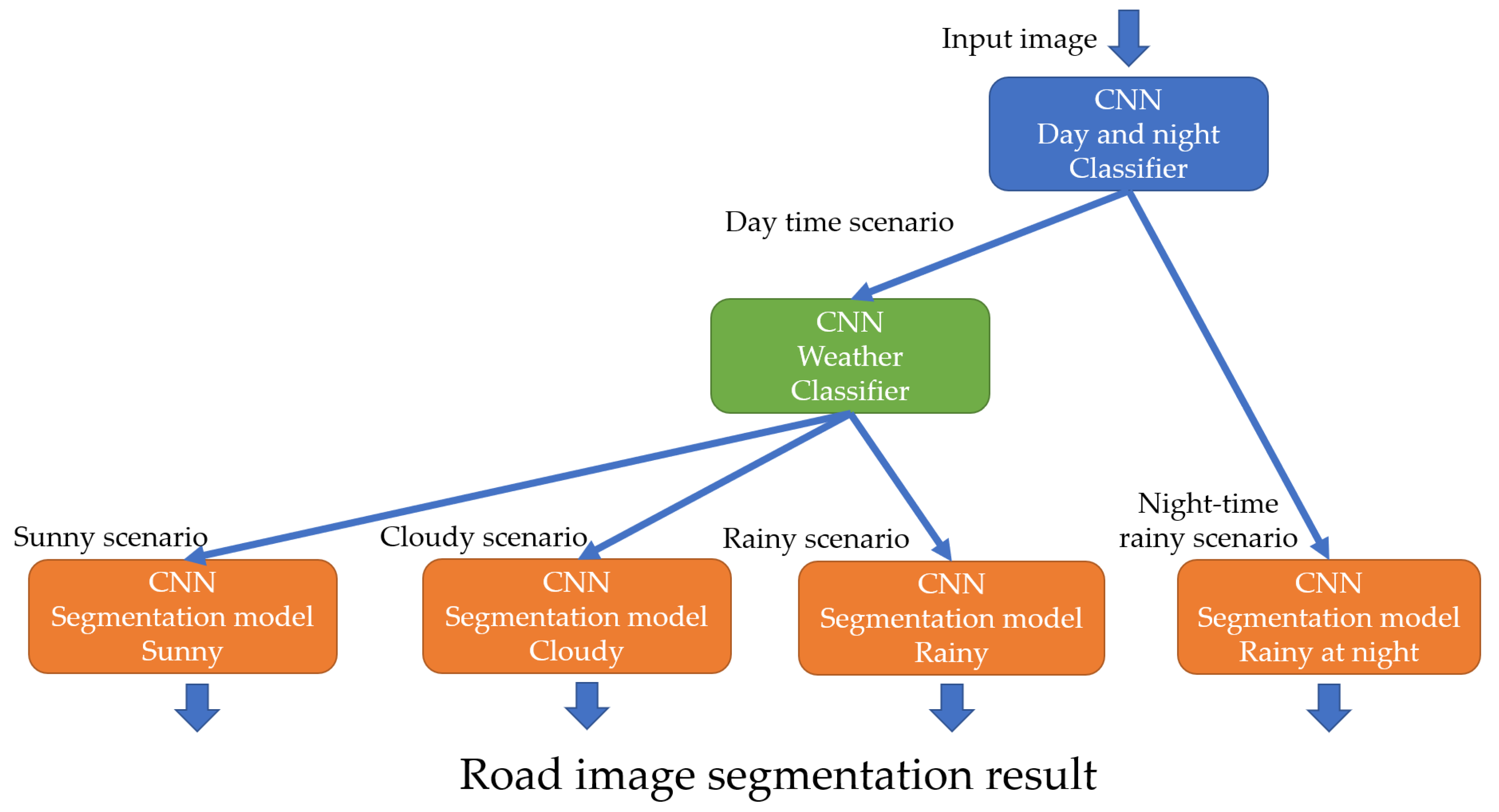
3.1. Model-Switching Architecture

Multi-model [46,47,48,49,50] is now a popular method in different applications. To accommodate multiple scenarios for road semantic segmentation, data from diverse situations must be used during model training. However, weights are affected by mutual suppression when a training model uses multiple scenarios, which reduces accuracy. Therefore, we used a model-switching architecture to eliminate the mutual suppression of weights.

Figure 2 presents an example of this architecture that uses a heuristic decision tree to switch between models for different scenarios. The gray nodes (D, E, F, and G) represent models in the neural network, and the orange (B and C) and blue (A) nodes represent the CNN classifiers that are used to select the model for segmentation.

3.2. Lightweight Processes

To increase the execution speed and maintain accuracy, lightweight processes, as de-tailed in this section, were used to reduce the computational load of the CNN.

3.2.1. Separable Convolution

We employed the concept of a separable convolution, which was first used in MobileNet [9]. To demonstrate the resulting reduction in computational load, we compared conventional convolution illustrated with separable convolution illustrated in Figure 3.

Conventional convolution computing consumption:

D_K·D_K·M·N·D_F·D_F

(1)

Separable convolution computing consumption:

D_K·D_K·M·D_F·D_F + M·N·D_F·D_F

(2)

D_K: Dimension of convolutional kernel. M: Number of input data channels. N: Number of output data channels. D_F: Dimension of output data feature.

The reduction in computation:

$$\frac{\mathrm{Separable} \mathrm{Convolution}}{\mathrm{Conventional} \mathrm{Convolution}} = \frac{{\mathrm{D}}_{\mathrm{K}}·{\mathrm{D}}_{\mathrm{K}}·\mathrm{M}·{\mathrm{D}}_{\mathrm{F}} ·{\mathrm{D}}_{\mathrm{F}}+\mathrm{M}·\mathrm{N}·{\mathrm{D}}_{\mathrm{F}} ·{\mathrm{D}}_{\mathrm{F}}}{{\mathrm{D}}_{\mathrm{K}}·{\mathrm{D}}_{\mathrm{K}}·\mathrm{M}·\mathrm{N}·{\mathrm{D}}_{\mathrm{F}} ·{\mathrm{D}}_{\mathrm{F}}} = \frac{1}{\mathrm{N}}+\frac{1}{{\mathrm{D}}_{\mathrm{K}}^2}$$

For the examples in Figure 3, the computation that is required for separable convolution is around 4.4% of that which is required for conventional convolution.

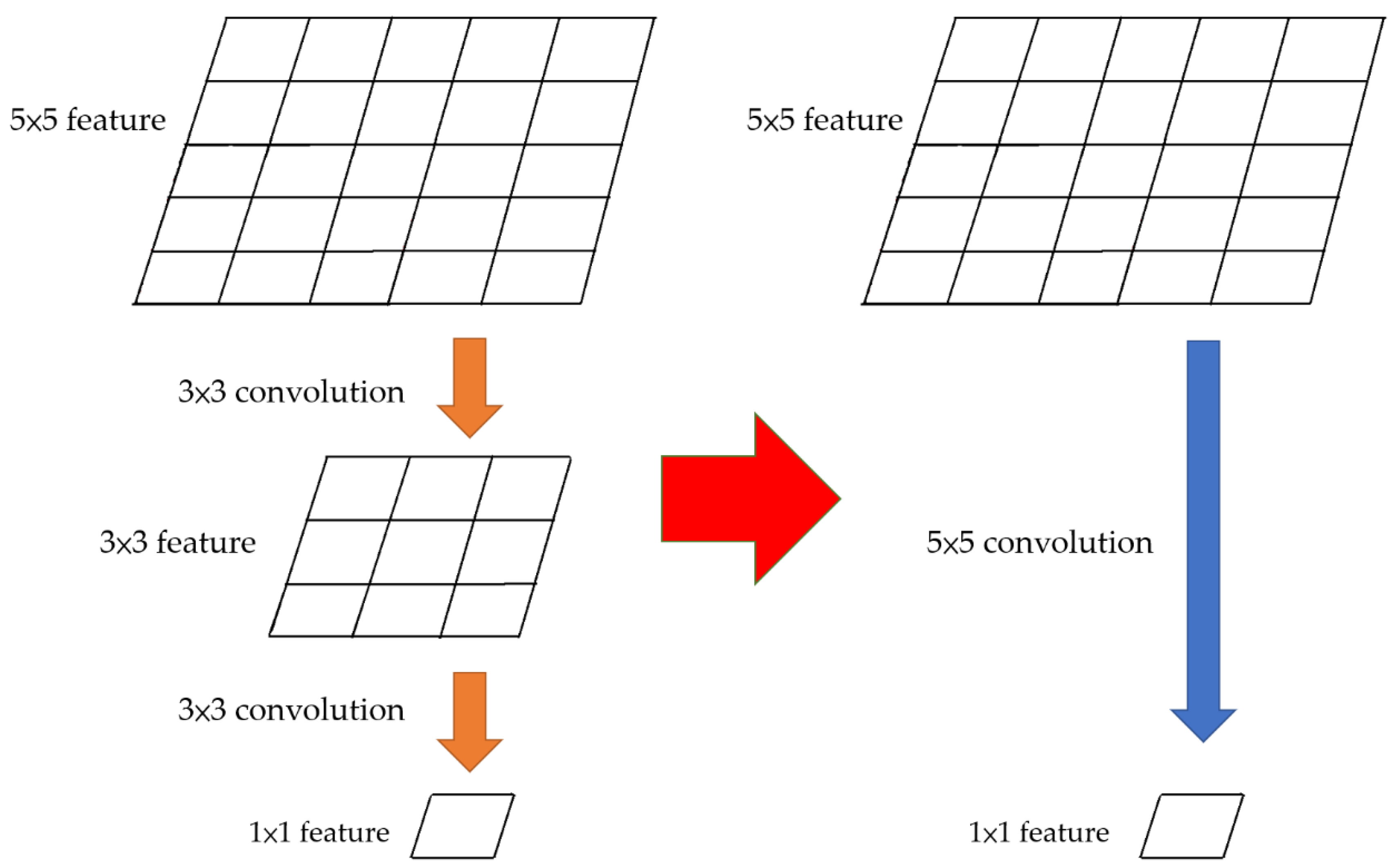
3.2.2. Reduction in Convolutional Layers

We employed the concept used in InceptionNet V3 [51] to reduce the number of layers in the original CNN to lower the weights and the amount of calculation, as well as to increase the execution speed of the CNN. The method for reducing the number of convolutional layers is depicted in Figure 4.

The number of 3 × 3 layers that is reduced into a single layer is calculated as:

((3·n) – (n – 1)) × ((3·n) – (n – 1))

(3)

n: Number of 3 × 3 layers.

The N × N convolution and M × M convolution that can be combined into a single layer is calculated as:

(N + M − 1) × (N + M − 1)

(4)

The computational loads for n-layered 3 × 3 convolution and single convolution by using Equations (1) and (2) are as follows:

n layered 3 × 3 conventional convolution:

$${{\displaystyle \sum }}_{\mathrm{i}=1}^{\mathrm{n}}{\mathrm{D}}_{\mathrm{Ki}}·{\mathrm{D}}_{\mathrm{Ki}}·{\mathrm{M}}_{\mathrm{i}}·{\mathrm{N}}_{\mathrm{i}}·{\mathrm{D}}_{\mathrm{Fi}}·{\mathrm{D}}_{\mathrm{Fi}}$$

One ((3·n) – (n – 1)) × ((3·n) – (n – 1)) conventional convolution:

D_KR·D_KR·M·N·D_FR·D_FR

One ((3·n) – (n – 1)) × ((3·n) – (n – 1)) separable convolution:

(D_KR·D_KR·M·D_FR·D_FR) + (M·N·D_FR·D_FR)

D_KR: ((3·N) – (N – 1)). D_FR: The feature dimension after kernel convolution. M: Number of input data channels. N: Number of output data channels. n: Number of 3 × 3 layers.

According to Equation (3), the two layered 3 × 3 convolution with 64 channels can be substituted by a single 5 × 5 convolution, which could reduce the computational cost by 87.7%, and by replacing two conventional convolutions with a separable convolution we could reduce the computational cost by 99.3%.

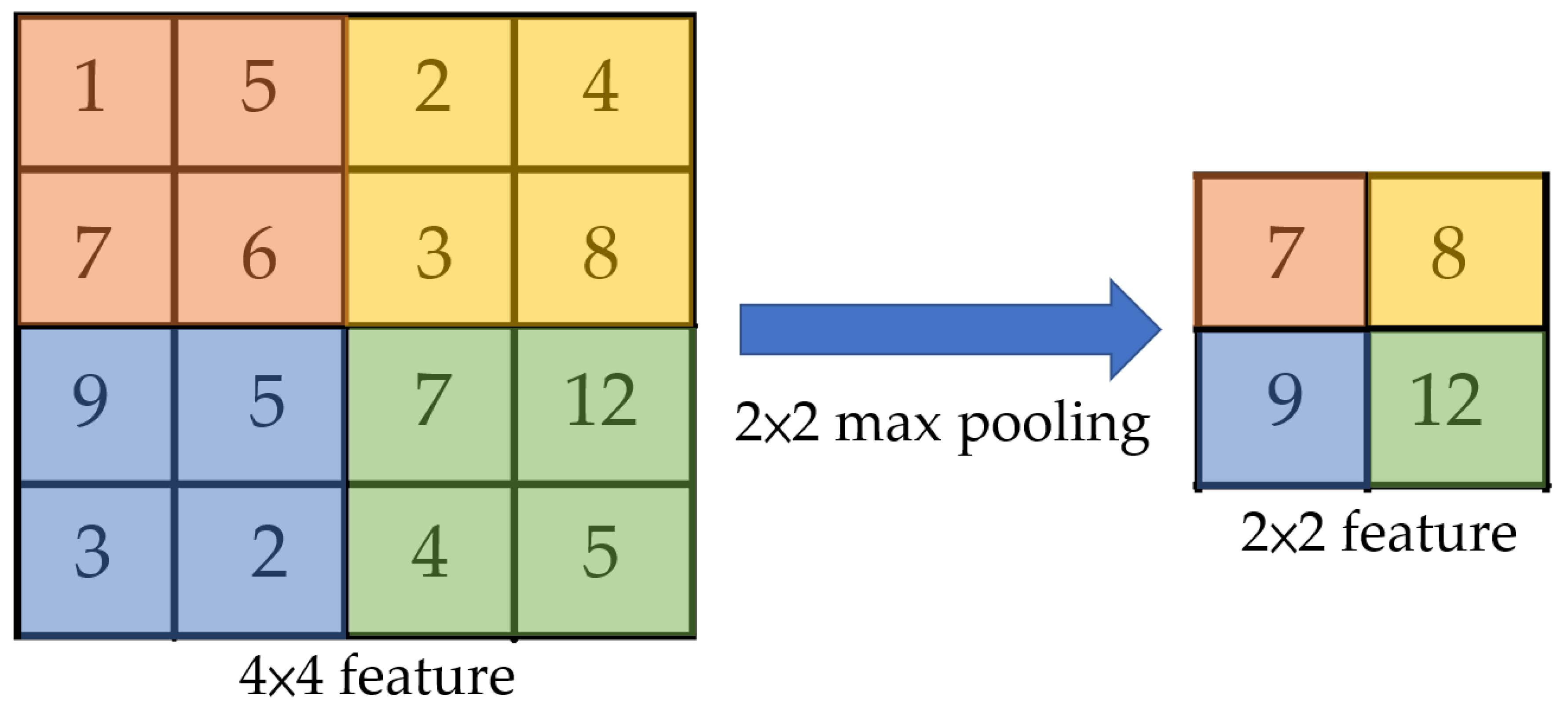
3.2.3. Remove Max Pooling and Maintain Output Size

To retain the detailed features of an image for increasing the accuracy of semantic segmentation and to reduce the computational cost for increasing the execution speed of the CNN, we eliminated the max pooling layers and changed the number of convolutional strides to maintain the output size after max pooling. The 2 × 2 max pooling operation is depicted in Figure 5. Max pooling selects the largest value in the mask; thus, sharper features in an image are retained, but the information that is not sharp is lost. The feature map after max pooling was half the size of the original feature map (Figure 6). The number of strides in the convolution was adjusted accordingly to reduce the computation cost and increase the execution speed.

4. Experiment

Experiments were conducted to validate the proposed model. A model with the proposed model-switching architecture was constructed. We used VGG as the CNN classifier for model selection and the FCN for semantic segmentation.

4.1. Hardware and Software Platform

For this study, our computer configuration was as show in

Table 1. Experiment computer configuration.

Configuration
GPU	RTX2080TI
CPU	Intel Xeon E5-2620
Motherboard	X79
Memory	DDR3 64 GB 1333 Hz
Operation system	Ubuntu 18.04
Programing language	Python 3.6
Machine learning library	TensorFlow 1.14

.

4.2. Model-Switching Architecture with Classifiers

In the experiment, we used four driving scenarios: rainy, sunny, cloudy, and rainy at night. Figure 7 illustrates the topology of the architecture. Two classifiers, namely, the day-and-night classifier and the weather classifier, were used to select the CNN model for performing semantic segmentation in various scenarios. The model-switching architecture used in this study is depicted in Figure 7. It used VGG16 as the day-and-night classifier (blue) and the weather classifier (green) to select a suitable CNN for semantic segmentation.

Identifying weather conditions and determining whether it is day or night is challenging. For these reasons, we employed a CNN classifier to realize model switching. Figure 8 presents the operation of the CNN classifier in scenario detection. Figure 9 depicts the model selection mechanism. By using the day-and-night classifier, the network selected an appropriate model for the time of the day; subsequently, by using the weather classifier, the network selected an appropriate model for the given weather scenario to perform road semantic segmentation.

4.3. Lightweight Fully Convolutional Neural Network

Figure 10 illustrates the conventional VGG16 that was used in our experiments. VGG16 is portable, accurate, and easy to modify. However, it is excessively large and requires considerable calculations. Thus, the lightweight processes that were previously described were incorporated into VGG16 to obtain a lightweight fast VGG (LWF-VGG). We used the VGG16 classifier for classification, VGG16 FCN for semantic segmentation, and lightweight VGG16 to construct a lightweight classifier and FCN.

To reduce the CNN size and the computational load, we replaced the conventional convolutions in VGG16 with separable convolutions, as illustrated in Figure 11. This change decreased the size of VGG16 from 1.6 GB to 235MB, or by 86%.

Using Equation (3), the number of convolutional layers in VGG16 can be reduced as displayed in Figure 11. This reduction from the original 22 to 12 layers reduced the size of VGG16 to 226 MB.

To further reduce the computational load, we removed the max pooling layers (Figure 11). The number of strides of the remaining separable convolutional layers was changed to 2 to ensure the same output as that obtained with 2 × 2 max pooling layers but with a slightly higher accuracy and faster execution speed. To reduce the computational load and accelerate computation speed, we also used the theorem in Equation 4 to build LWF-VGG tiny.

4.4. Experimental Results

The proposed FCN with a model-switching architecture and LWF-VGG was used for road semantic segmentation for different scenarios.

4.4.1. Comparison of Various Methods in Semantic Segmentation

To test the performance, we used the KITTI road dataset which is widely used for road semantic segmentation research. It comprised 289 training images with a resolution of 1242 × 375. We also performed a NTUT sunny dataset, NTUT cloudy dataset, NTUT rainy dataset and NTUT night rainy dataset. Each of them comprised 250 training images with a resolution of 1920 × 1080. Figure 12 shows the road segmentation results for the datasets using LWF-VGG FCN.

Table 2. Performance of different neural networks using the KITTI road dataset. Max: maximum; Avg: average; PRE: precision; REC: recall.

Method	Input	Max F1-Score	Avg PRE	Max PRE	REC
VGG16 FCN	Image	0.9243	0.9810	1.0000	0.8779
StixelNet II	Image	0.9488	0.8775	0.9297	0.9687
MultiNet	Image	0.9488	0.9371	0.9484	0.9491
RBNet	Image	0.9497	0.9149	0.9494	0.9501
LidCamNet	Image + LiDAR	0.9603	0.9393	0.9623	0.9583
NF2CNN	Image + LiDAR	0.9670	0.8993	0.9537	0.9807
PSPNet	Image	0.9629	0.9371	0.9622	0.9635
PLARD+	Image + LiDAR	0.9703	0.9403	0.9719	0.9688
SNE-RoadSeg+	RGB-D	0.9740	0.9401	0.9801	0.9749
LWF-VGG FCN tiny	Image	0.9741	0.973	0.978	0.9751
LWF-VGG FCN	Image	0.9745	0.9655	1.0000	0.9845

shows the performance of the various approaches in the KITTI dataset. Image-based, image + RGB-D based, and image + LiDAR-based approaches had a comparable performance. However, image-based approaches incur a lower equipment cost and the techniques can be more easily realized. To solve different driving scenarios in Taiwan and show the performance of our approach, we used four different datasets for testing.

Table 3. Performance of different approaches using the various road datasets. Avg: average; IOU: intersection over union; REC: recall; PRE: precision; FPS: frame per second.

NTUT Sunny	Size	Avg IOU	Avg REC	Avg PRE	Avg F1-Score	FPS
MultiNet	1.2 GB	0.971	0.962	0.975	0.979	0.91
VGG16-FCN	1.6 GB	0.987	0.980	0.980	0.980	0.87
BiSeNet	207 MB	0.908	0.894	0.921	0.907	2.89
BiSeNet V2	45.9 MB	0.956	0.942	0.925	0.955	3.09
LWF-VGG FCN tiny	29 MB	0.985	0.979	0.981	0.977	2.87
LWF-VGG-FCN	226 MB	0.987	0.980	0.980	0.981	1.77
NTUT cloudy
MultiNet	1.2 GB	0.959	0.948	0.961	0.964	0.91
VGG16-FCN	1.6 GB	0.967	0.976	0.976	0.976	0.87
BiSeNet	207 MB	0.890	0.906	0.904	0.912	2.89
BiSeNet V2	45.9 MB	0.937	0.954	0.952	0.961	3.09
LWF-VGG FCN tiny	29 MB	0.970	0.974	0.977	0.975	2.87
LWF-VGG-FCN	226 MB	0.972	0.978	0.981	0.980	1.77
NTUT rainy
MultiNet	1.2 GB	0.795	0.778	0.802	0.811	0.91
VGG16-FCN	1.6 GB	0.850	0.780	0.913	0.831	0.87
BiSeNet	207 MB	0.774	0.792	0.806	0.809	2.89
BiSeNet V2	45.9 MB	0.815	0.804	0.811	0.852	3.09
LWF-VGG FCN tiny	29 MB	0.942	0.944	0.940	0.936	2.87
LWF-VGG-FCN	226 MB	0.945	0.945	0.941	0.939	1.77
NTUT night rainy
MultiNet	1.2 GB	0.933	0.912	0.934	0.941	0.91
VGG16-FCN	1.6 GB	0.940	0.959	0.959	0.965	0.87
BiSeNet	207 MB	0.904	0.914	0.907	0.913	2.89
BiSeNet V2	45.9 MB	0.952	0.963	0.955	0.962	3.09
LWF-VGG FCN tiny	29 MB	0.970	0.974	0.980	0.976	2.87
LWF-VGG-FCN	226 MB	0.977	0.986	0.989	0.987	1.77

shows the performance in different scenarios and a comparison of different approaches.

Figure 12 shows the road semantic segmentation results of LWF-VGG FCN for the sunny scenario in the KITTI dataset and NTUT Sunny dataset. The performance in the KITTI dataset of LWF-VGG FCN and LWF-VGG FCN tiny were very close to the modern state of the arts. For the maximum F -score and maximum precision, LWF-VGG FCN had better performance compared to the others. For recall, LWF-VGG FCN tiny had better performance compared to the others. The KITTI dataset is a widely used dataset in the field of road semantic segmentation. However, it’s not suitable for Taiwanese road scenarios with various climates. To validate its applicability to road semantic segmentation in Taiwan, the proposed FCNs were tested using a dataset for road conditions in Taipei City, which was collected by the National Taiwan University of Technology (NTUT). The NTUT dataset comprised four sets of images for different weather conditions and times of day: sunny, cloudy, rainy, and night rainy. According to the scenarios named the NTUT sunny dataset, NTUT cloudy dataset, NTUT rainy dataset, and night rainy dataset, respectively, to show the performance of LWF-VGG tiny, we used the state of the art methods called MultiNet [34], BiSeNet [52], and BiSeNet v2 [53] to obtain a comparison.

Table 3 shows the performance of LWF-VGG FCN and LWF-VGG FCN tiny compared with different approaches. The NTUT rainy dataset was the most challenging dataset of our driving scenario. Due to the reflection and refraction on the surface, the feature of the road image became complicated. To retain the complicated features of the rainy road image, LWF-VGG FCN and LWF-VGG FCN tiny used the theorem from Section 3.2.3 which removed the max pooling and changed the convolution strides to maintain the output size. This method could solve the complicated feature in rainy day. It also reduced the computational load and accelerating computation speed. LWF-VGG FCN tiny had approaching inference speed compared to the state of the arts.

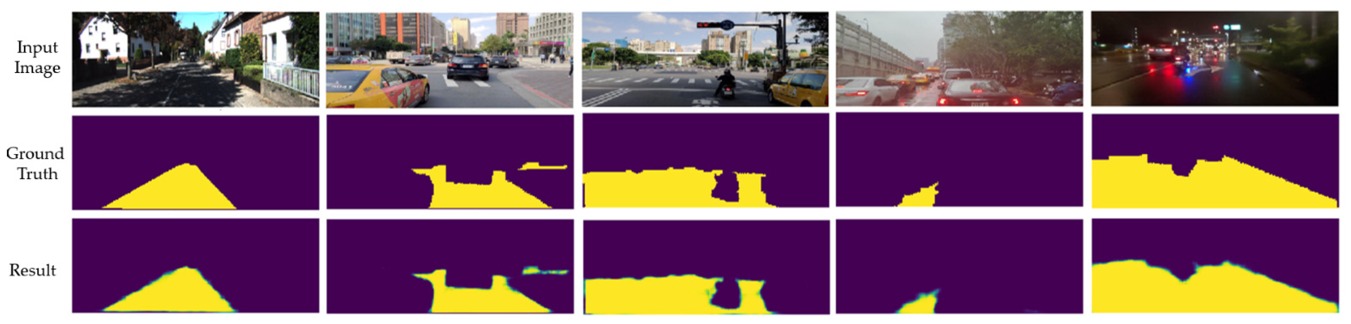
4.4.2. Multi-Scenario Road Semantic Segmentation with Model-Switching Architecture

In real-world applications, road conditions change constantly. To determine whether the proposed FCN with the model-switching architecture adapts to changing conditions, we combined the four sets of images into a mixed dataset of 1000 images with a resolution of 1920 × 1080 and called it the NTUT mixed dataset. The test results obtained for the NTUT mixed dataset are depicted in Figure 13. To switch the proper model for road image segmentation, we needed to train the classifiers. Collecting training data and labeling is hard work that requires a significant amount of time and human work. To reduce the human work and time consumption, the few-shot image classification is important research now. The day–night dataset consisted of 207 day-time images and 86 night-time images. The weather dataset used for weather classification consisted of 190 cloudy scenario images, 173 rainy scenario images, and 240 sunny scenario images. In

Table 4. Accuracy of VGG16, LWF-VGG, and LWF-VGG tiny as classifiers. Avg: average.

Day and Night	Day	Night		Avg	Model Size
VGG16	0.9992	0.9980		0.9986	1.6 GB
LWF-VGG-tiny	0.9976	0.9792		0.9884	32 MB
LWF-VGG	0.9989	0.9984		0.9986	230 MB
Weather	Sunny	Cloudy	Rainy
VGG16	0.9955	0.9981	0.969	0.9875	1.6 GB
LWF-VGG-tiny	0.9940	0.9912	0.974	0.9864	32 MB
LWF-VGG	0.9954	0.9951	0.980	0.9902	230 MB

, the model size and recognition accuracy of VGG16 and LWF-VGG as classifiers were compared at different times of day and under distinct weather conditions. The image recognition accuracy was comparable for different scenarios, but the model size of LWF-VGG was considerably smaller at only approximately 14% of the model size of VGG16.

The left side of Figure 13 shows the semantic segmentation results obtained using the LWF-VGG FCN after training with the NTUT mixed dataset. The right side of Figure 13 shows the results obtained using multiple LWF-VGG FCNs that were trained using various datasets in different contexts and then switched to a suitable model for semantic segmentation by using the model-switching architecture. To demonstrate the effectiveness of the model-switching architecture, we trained one LWF-VGG FCN by using the NTUT mixed dataset and trained four LWF-VGG FCNs by using the NTUT sunny dataset, the NTUT cloudy dataset, the NTUT rainy dataset, and the NTUT night rainy dataset, respectively, and used the model-switching architecture to switch to a suitable model for semantic segmentation. A comparison of the results obtained using a single VGG16 FCN, multiple VGG16 FCNs with the model-switching architecture, a single LWF-VGG FCN, and multiple LWF-VGG FCNs with the model-switching architecture is presented in

Table 5. Multi-model and single-model testing using the NTUT mixed dataset. Avg: average; IOU: intersection over union; REC: recall; PRE: precision; FPS: frame per second.

Multi-Model/Single-Model	Avg IOU	Avg REC	Avg PRE	Avg F1-Score	FPS
Single-model VGG16 FCN	0.853	0.844	0.862	0.861	0.89
Single-model LWF-VGG FCN tiny	0.883	0.878	0.903	0.897	2.96
Single-model LWF-VGG FCN	0.891	0.884	0.902	0.903	1.80
Multi-model VGG16 FCNs	0.908	0.898	0.928	0.910	0.75
Multi-model LWF-VGG FCNs tiny	0.937	0.953	0.947	0.947	2.51
Multi-model LWF-VGG FCNs	0.949	0.952	0.951	0.952	1.53

.

Table 5 presents a comparison of multiple CNNs with their own weights and model-switching architectures with that of a single CNN with multiple weights. Both the multiple VGG16 FCNs and multiple LWF-VGG FCNs outperformed the single VGG16 FCN and single LWF-VGG FCN, and the multiple LWF-VGG FCNs with the model-switching architecture were faster than the single VGG16 FCN. LWF-VGG FCNs tiny were even faster.

5. Conclusions

The proposed model-switching architecture prevents mutual suppression between weights in a single CNN model. This architecture uses multiple CNN models to store the weights of various states individually and uses one or more CNN classifiers to identify the current state and switch to a suitable model for semantic segmentation.

However, the model-switching architecture and semantic segmentation require considerable computation, resulting in time delays. Therefore, we proposed a simple but effective light-weight CNN method to increase the calculation speed. The execution speed was limited by the memory bandwidth in this experiment. Nevertheless, it was approximately two times faster than that of the original method. The proposed method was particularly effective for VGG-like CNNs.

This paper used FCN for semantic segmentation which is the pioneer in field of semantic segmentation. However, the architecture was limited to the aspect ratio of the input images. Additionally, we plan to conduct bilateral network research on semantic segmentation deep learning in the future.

References

1. Alex, K.; Ilya, S.; Geoffrey, E.H. ImageNet Classification with Deep Convolutional Neural Networks. Adv. Neural Inf. Process. Syst. 2012, 25, 1097–1105. [Google Scholar]
2. He, K.; Zhang, X.; Ren, S.; Sun, J. Deep Residual Learning for Image Recognition. arXiv 2015, arXiv:1512.03385. [Google Scholar]
3. Xie, S.; Girshick, R.; Dollár, P.; Tu, Z.; He, K. Aggregated Residual Transformations for Deep Neural Networks. arXiv 2017, arXiv:1611.05431v2. [Google Scholar]
4. Gao, S.; Cheng, M.; Zhao, K.; Zhang, X.; Yang, M.; Philip, T. Res2Net: A New Multi-scale Backbone Architecture. arXiv 2019, arXiv:1904.01169v3. [Google Scholar] [CrossRef] [Green Version]
5. Zoph, B.; Le, Q.V. Neural Architecture Search with Reinforcement Learning. arXiv 2016, arXiv:1611.01578v2. [Google Scholar]
6. Zoph, B.; Vasudevan, V.; Shlens, J.; Le, Q.V. Learning Transferable Architectures for Scalable Image Recognition. arXiv 2018, arXiv:1707.07012v4. [Google Scholar]
7. Liu, C.; Zoph, B.; Neumann, M.; Shlens, J.; Hua, W.; Li, L.J.; Li, F.F.; Yuille, A.; Huang, J.; Murphy, K. Progressive Neural Architecture Search. arXiv 2018, arXiv:1712.00559v3. [Google Scholar]
8. Tan, M.; Chen, B.; Pang, R.; Vasudevan, V.; Sandler, M.; Howard, A.; Le, Q.V. MnasNet: Platform-Aware Neural Architecture Search for Mobile. arXiv 2019, arXiv:1807.11626v3. [Google Scholar]
9. Howard, A.G.; Zhu, M.; Chen, B.; Kalenichenko, D.; Wang, W.; Weyand, T.; Andreetto, M.; Adam, H. MobileNets: Efficient Convolutional Neural Networks for Mobile Vision Applications. arXiv 2017, arXiv:1704.04861v1. [Google Scholar]
10. Mark, S.; Andrew, H.; Zhu, M.; Andrey, Z.; Chen, L.C. MobileNetV2: Inverted Residuals and Linear Bottlenecks. arXiv 2018, arXiv:1801.04381v4. [Google Scholar]
11. Howard, A.; Sandler, M.; Chu, G.; Chen, L.C.; Chen, B.; Tan, M.; Wang, W.; Zhu, Y.; Pang, R.; Vasudevan, V.; et al. Searching for MobileNetV3. arXiv 2019, arXiv:1905.02244v5. [Google Scholar]
12. Zhang, X.; Zhou, X.; Lin, M.; Sun, J. ShuffleNet: An Extremely Efficient Convolutional Neural Network for Mobile Devices. arXiv 2017, arXiv:1707.01083v2. [Google Scholar]
13. Ma, N.; Zhang, X.; Zheng, H.T.; Sun, J. ShuffleNet V2: Practical Guidelines for Efficient CNN Architecture Design. arXiv 2018, arXiv:1807.11164v1. [Google Scholar]
14. Tan, M.; Le, Q.V. EfficientNet: Rethinking Model Scaling for Convolutional Neural Networks. arXiv 2019, arXiv:1905.11946v3. [Google Scholar]
15. Tan, M.; Le, Q.V. EfficientNetV2: Smaller Models and Faster Training. arXiv 2021, arXiv:2104.00298v3. [Google Scholar]
16. Long, J.; Shelhamer, E.; Darrell, T. Fully Convolutional Networks for Semantic Segmentation, Computing. arXiv 2015, arXiv:1411.4038v2. [Google Scholar]
17. Vijay, B.; Alex, K.; Roberto, C. SegNet: A Deep Convolutional Encoder-Decoder Architecture for Image Segmentation. arXiv 2015, arXiv:1511.00561v3. [Google Scholar]
18. Ronneberger, O.; Fischer, P.; Brox, T. U-Net: Convolutional Networks for Biomedical Image Segmentation. arXiv 2015, arXiv:1505.04597v1. [Google Scholar]
19. Fausto, M.; Nassir, N.; Ahmadi, S. V-Net: Fully Convolutional Neural Networks for Volumetric Medical Image Segmentation. arXiv 2016, arXiv:1606.04797v1. [Google Scholar]
20. Zhou, Z.; Siddiquee, M.; Tajbakhsh, N.; Liang, J. UNet++: Redesigning Skip Connections to Exploit Multiscale Features in Image Segmentation. IEEE Trans. Med. Imaging 2020, 39, 1856–1867. [Google Scholar] [CrossRef] [PubMed] [Green Version]
21. Zhao, H.; Jiang, L.; Jia, J.; Philip, T.; Vladlen, K. Point Transformer. arXiv 2020, arXiv:2012.09164v1. [Google Scholar]
22. Guo, M.; Cai, J.; Liu, Z.; Mu, T.; Ralph, R.M.; Hu, S. PCT: Point cloud transformer. arXiv 2021, arXiv:2012.09688v4. [Google Scholar]
23. Liu, Z.; Lin, Y.; Cao, Y.; Hu, H.; Wei, Y.; Zhang, Z.; Lin, S.; Guo, B. Swin Transformer: Hierarchical Vision Transformer using Shifted Windows. arXiv 2021, arXiv:2103.14030v1. [Google Scholar]
24. Zhao, H.; Shi, J.; Qi, X.; Wang, X.; Jia, J. Pyramid Scene Parsing Network. arXiv 2017, arXiv:1612.01105v2. [Google Scholar]
25. Yang, M.; Yu, K.; Zhang, C.; Li, Z.; Yang, K. DenseASPP for Semantic Segmentation in Street Scenes. In Proceedings of the IEEE Conference on Computer Vision and Pattern Recognition, Salt Lake City, UT, USA, 18–23 June 2018. [Google Scholar]
26. Chen, L.C.; Papandreou, G.; Kokkinos, I.; Murphy, K.; Yuille, A.L. Semantic Image Segmentation with Deep Convolutional Nets and Fully Connected CRFS. arXiv 2016, arXiv:1412.7062v4. [Google Scholar]
27. Chen, L.C.; Papandreou, G.; Kokkinos, I.; Murphy, K.; Yuille, A.L. DeepLab: Semantic Image Segmentation with Deep Convolutional Nets, Atrous Convolution, and Fully Connected CRFs. arXiv 2017, arXiv:1606.00915v2. [Google Scholar] [CrossRef]
28. Chen, L.C.; Papandreou, G.; Schroff, F.; Adam, H. Rethinking Atrous Convolution for Semantic Image Segmentation. arXiv 2017, arXiv:1706.05587v3. [Google Scholar]
29. Chen, L.C.; Zhu, Y.; Papandreou, G.; Schroff, F.; Adam, H. Encoder-Decoder with Atrous Separable Convolution for Semantic Image Segmentation. arXiv 2018, arXiv:1802.02611v3. [Google Scholar]
30. Caio, C.; Vincent, F.; Denis, F. Vision-Based Road Detection using Contextual Blocks. arXiv 2015, arXiv:1509.01122v1. [Google Scholar]
31. Rahul, M. Deep Deconvolutional Networks for Scene Parsing. arXiv 2014, arXiv:1411.4101v1. [Google Scholar]
32. Chen, Z.; Chen, Z. RBNet: A Deep Neural Network for Unified Road and Road Boundary Detection. In Proceedings of the 24th International Conference on Neural Information Processing, Guangzhou, China, 14–18 November 2017. [Google Scholar]
33. Caio, C.; Vincent, F.; Denis, F. Exploiting Fully Convolutional Neural Networks for Fast Road Detection. In Proceedings of the 2016 IEEE International Conference on Robotics and Automation, Stockholm, Sweden, 16–21 May 2016. [Google Scholar]
34. Marvin, T.; Michael, W.; Marius, Z.; Roberto, C.; Raquel, U. MultiNet: Real-time Joint Semantic Reasoning for Autonomous Driving. In Proceedings of the 2018 IEEE Intelligent Vehicles Symposium, Changshu, China, 26–30 June 2018. [Google Scholar]
35. Ha, Q.; Watanabe, K.; Karasawa, T.; Ushiku, Y.; Harada, T. MFNet: Towards Real-Time Semantic Segmentation for Autonomous Vehicles with Multi-Spectral Scenes. In Proceedings of the 2017 IEEE/RSJ International Conference on Intelligent Robots and Systems, Vancouver, BC, Canada, 24–28 September 2017. [Google Scholar]
36. Sun, J.Y.; Kim, S.W.; Lee, S.W.; Kim, Y.W.; Ko, S.J. Reverse and Boundary Attention Network for Road Segmentation. In Proceedings of the IEEE/CVF International Conference on Computer Vision Workshops, Seoul, Korea, 27–28 October 2019. [Google Scholar]
37. Shinzato, P.Y.; Denis, F.W.; Christoph, S. Road Terrain Detection: Avoiding Common Obstacle Detection Assumptions Using Sensor Fusion. In Proceedings of the IEEE Intelligent Vehicles Symposium, Dearborn, MI, USA, 8–11 June 2014. [Google Scholar]
38. Xiao, L.; Dai, B.; Liu, D.; Hu, T.; Wu, T. CRF based Road Detection with Multi-Sensor Fusion. In Proceedings of the 2015 IEEE Intelligent Vehicles Symposium, Seoul, Korea, 28 June–1 July 2015. [Google Scholar]
39. Gu, S.; Zhang, Y.; Tang, J.; Yang, J.; Kong, H. Road Detection through CRF based LiDAR-Camera Fusion. In Proceedings of the International Conference on Robotics and Automation, Montreal, QC, Canada, 20–24 May 2019. [Google Scholar]
40. Luca, C.; Mauro, B.; Lennart, S.; Mattias, W. LIDAR-Camera Fusion for Road Detection Using Fully Convolutional Neural Networks. arXiv 2018, arXiv:1809.07941v1. [Google Scholar]
41. Gu, S.; Zhang, Y.; Yang, J.; Jose, M.A.; Kong, H. Two-View Fusion based Convolutional Neural Network for Urban Road Detection. In Proceedings of the IEEE/RSJ International Conference on Intelligent Robots and Systems, The Venetian Macao, Macau, China, 4–8 November 2019. [Google Scholar]
42. Sun, Y.; Zuo, W.; Liu, M. RTFNet: RGB-Thermal Fusion Network for Semantic Segmentation of Urban Scenes. IEEE Robot. Autom. Lett. 2019, 4, 2576–2583. [Google Scholar] [CrossRef]
43. Fan, R.; Wang, H.; Cai, P.; Liu, M. SNE-RoadSeg: Incorporating Surface Normal Information into Semantic Segmentation for Accurate Freespace Detection. In European Conference on Computer Vision; Springer: Cham, Switzerland, 2020. [Google Scholar]
44. Chen, Z.; Zhang, J.; Tao, D. Progressive LiDAR Adaptation for Road Detection. J. Autom. Sin. 2019, 6, 693–702. [Google Scholar] [CrossRef] [Green Version]
45. Simonyan, K.; Zisserman, A. Very Deep Convolutional Networks for Large-Scale Image Recognition. arXiv 2015, arXiv:1409.1556v6. [Google Scholar]
46. Kowsari, K.; Heidarysafa, M.; Brown, D.E.; Meimandi, K.J.; Barnes, L.E. RMDL: Random Multimodel Deep Learning for Clas-sification. arXiv 2018, arXiv:1805.01890v2. [Google Scholar]
47. Tommasi, T.; Orabona, F.; Caputo, B. Learning Categories From Few Examples With Multi Model Knowledge Transfer. IEEE Trans. Pattern Anal. Mach. Intell. 2014, 36, 928–941. [Google Scholar] [CrossRef] [PubMed] [Green Version]
48. Yin, Q.; Zhang, R.; Shao, X. CNN and RNN mixed model for image classification. MATEC 2019, 277, 02001. [Google Scholar] [CrossRef]
49. Ding, C.; Tao, D. Robust Face Recognition via Multimodal Deep Face Representation. IEEE Trans. Multimed. 2015, 17, 2049–2058. [Google Scholar] [CrossRef]
50. Hong, D.; Gao, L.; Yokoya, N. More Diverse Means Better: Multimodal Deep Learning Meets Remote-Sensing Imagery Classi-fication. IEEE Trans. Geosci. Remote Sens. 2020, 59, 4340–4354. [Google Scholar] [CrossRef]
51. Szegedy, C.; Vanhoucke, V.; Ioffe, S.; Shlens, J.; Wojna, Z. Rethinking the Inception Architecture for Computer Vision. arXiv 2015, arXiv:1512.00567v3. [Google Scholar]
52. Yu, C.; Wang, J.; Peng, C.; Gao, C.; Yu, G.; Sang, N. BiSeNet: Bilateral Segmentation Network for Real-time Semantic Seg-mentation. In Proceedings of the European Conference on Computer Vision, Munich, Germany, 8–14 September 2018; pp. 325–341. [Google Scholar]
53. Yu, C.; Gao, C.; Wang, J.; Yu, G.; Shen, C. Sang, N. BiSeNet V2: Bilateral Network with Guided Aggregation for Real-time Semantic Segmentation. arXiv 2020, arXiv:2004.02147v1. [Google Scholar]
Figure 1. Proposed convolutional network with model-switching architecture and lightweight processes.
Applsci 11 07424 g001
Figure 2. An example of model-switching architecture.
Applsci 11 07424 g002
Figure 3. Conventional convolution and separable convolution.
Applsci 11 07424 g003
Figure 4. A 5 × 5 feature can be aggregated into 1 × 1 feature after two 3 × 3 convolutions or a 5 × 5 convolution.
Applsci 11 07424 g004
Figure 5. Operation of 2 × 2 max pooling on 4 × 4 feature.
Applsci 11 07424 g005
Figure 6. Convolution with a 2 × 2 kernel using convolutional stride 2 work on a 4 × 4 feature map.
Applsci 11 07424 g006
Figure 7. Topology of the model-switching architecture.
Applsci 11 07424 g007
Figure 8. Operation of the convolutional neural network classifier.
Applsci 11 07424 g008
Figure 9. Mechanism of model selection.
Applsci 11 07424 g009
Figure 10. (upper) VGG16 classifier (lower) VGG16 FCN.
Applsci 11 07424 g010
Figure 11. Light-weight process of VGG16.
Applsci 11 07424 g011
Figure 12. Road semantic segmentation results using LWF-VGG FCN.
Applsci 11 07424 g012
Figure 13. Road semantic segmentation result using model-switching architecture with the LWF-VGG FCNs and LWF-VGG FCN.
Applsci 11 07424 g013