
Integrating InSAR Observables and Multiple Geological Factors for Landslide Susceptibility Assessment


Abstract
:1. Introduction
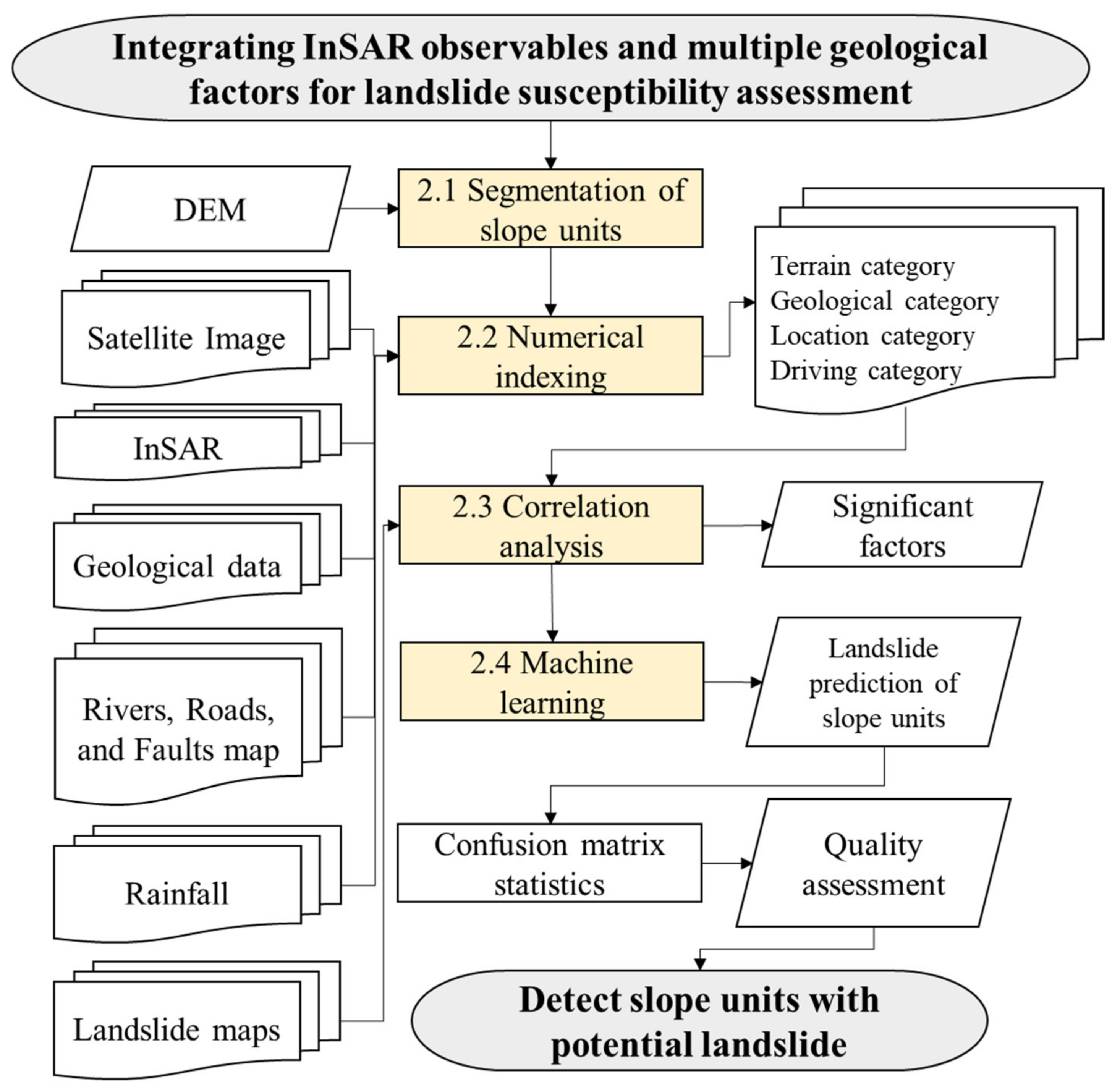
2. Methods
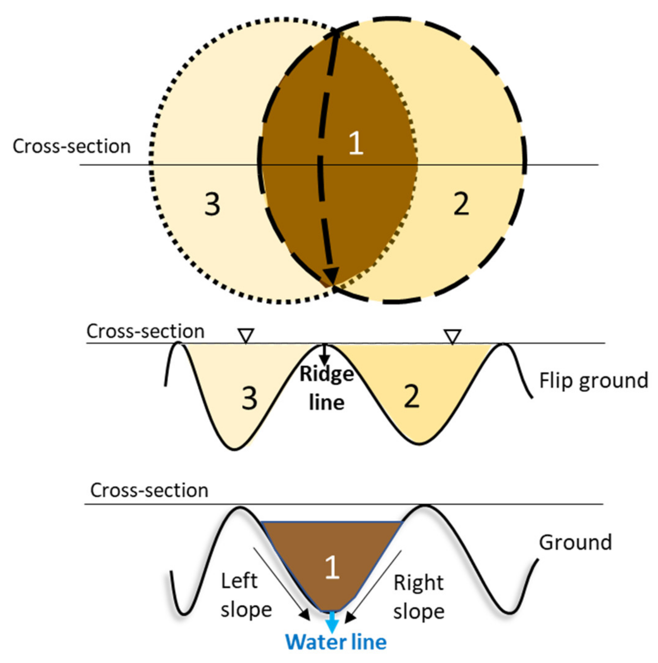
2.1. Segmentation of Slope Units
2.2. Numerical Indexing of Related Spatial Factors
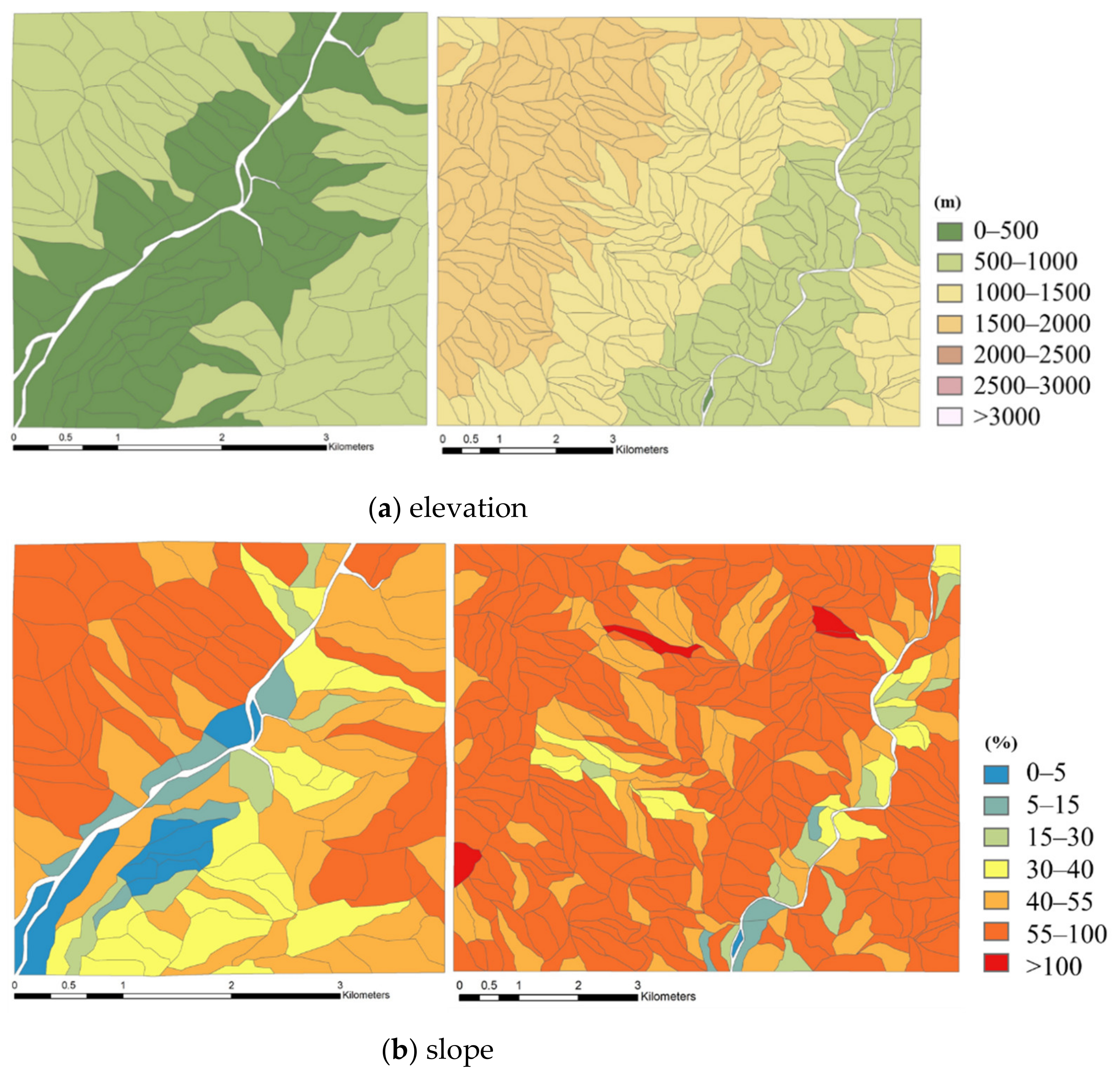
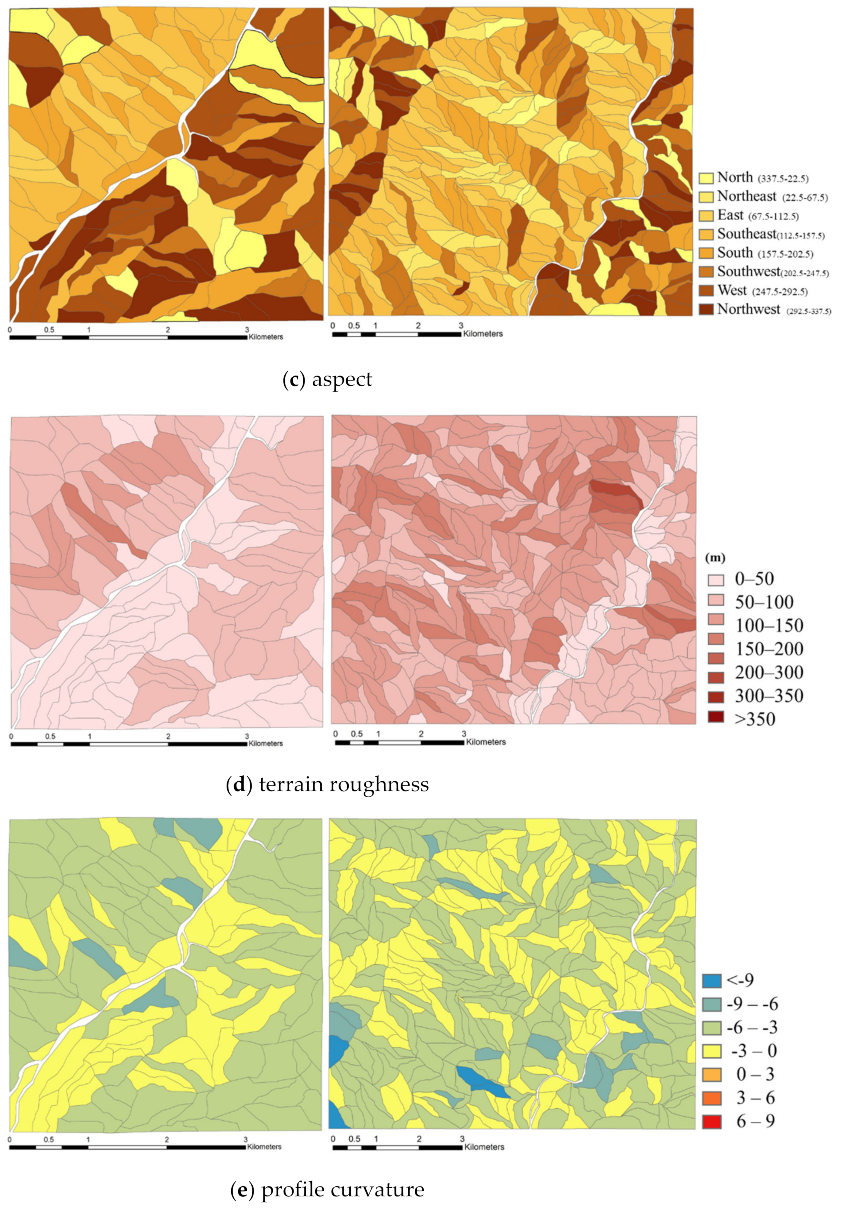
2.2.1. Terrain Category
- Elevation, slope, and aspect
- Terrain roughness
- Profile curvature
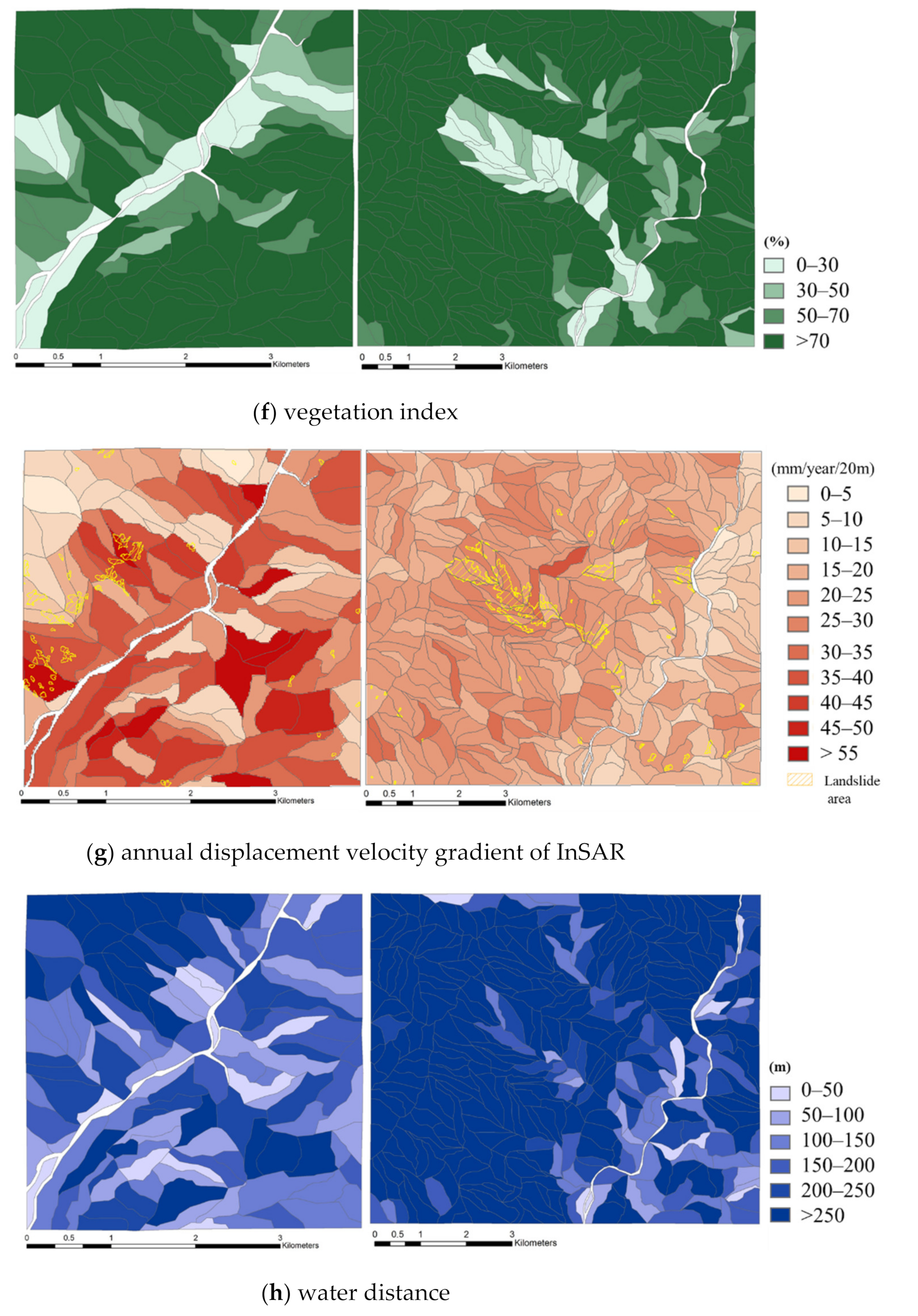
- Vegetation index
- Annual displacement velocity gradient of InSAR
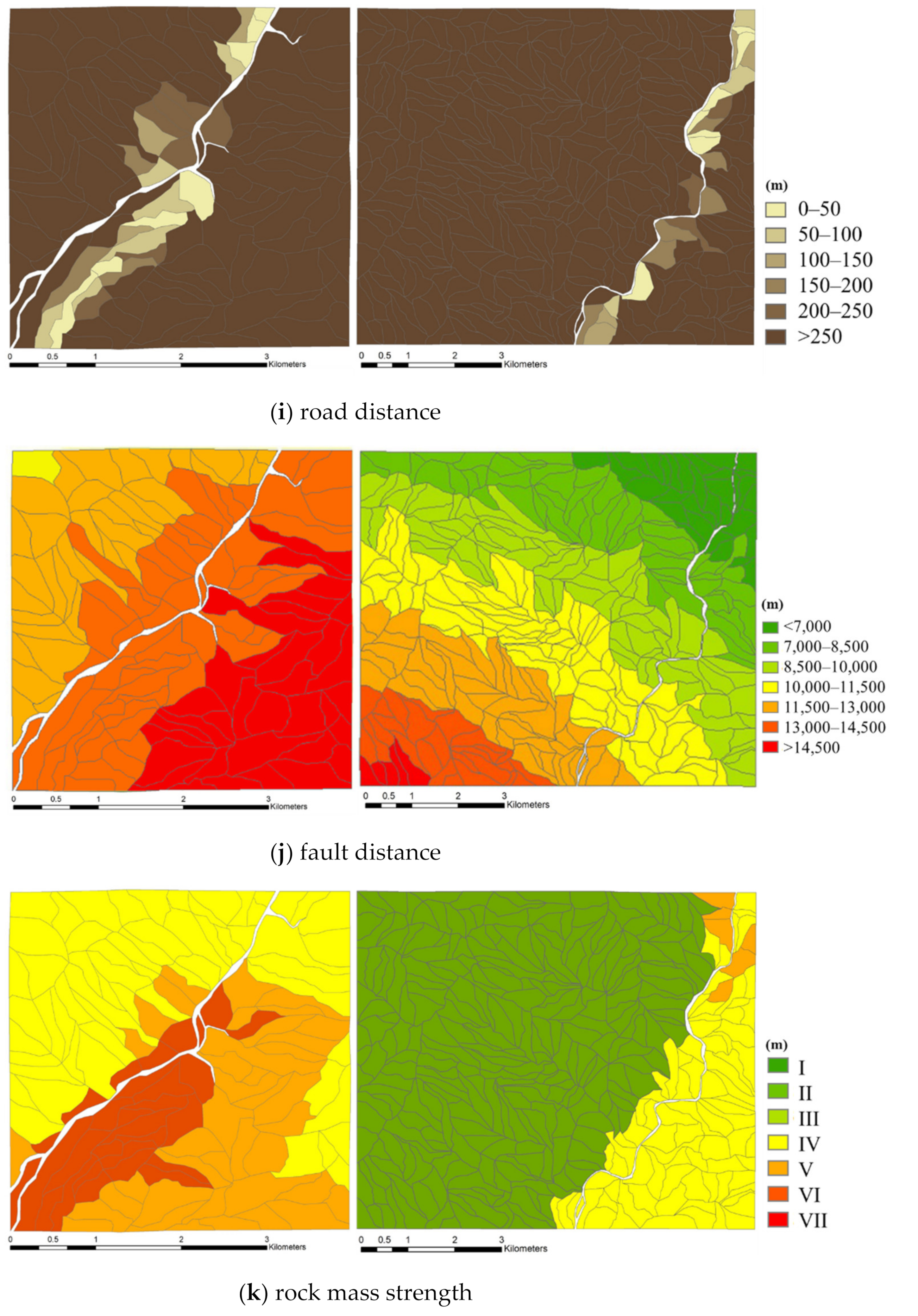
2.2.2. Location Category
2.2.3. Geological Category
- Rock Mass Strength
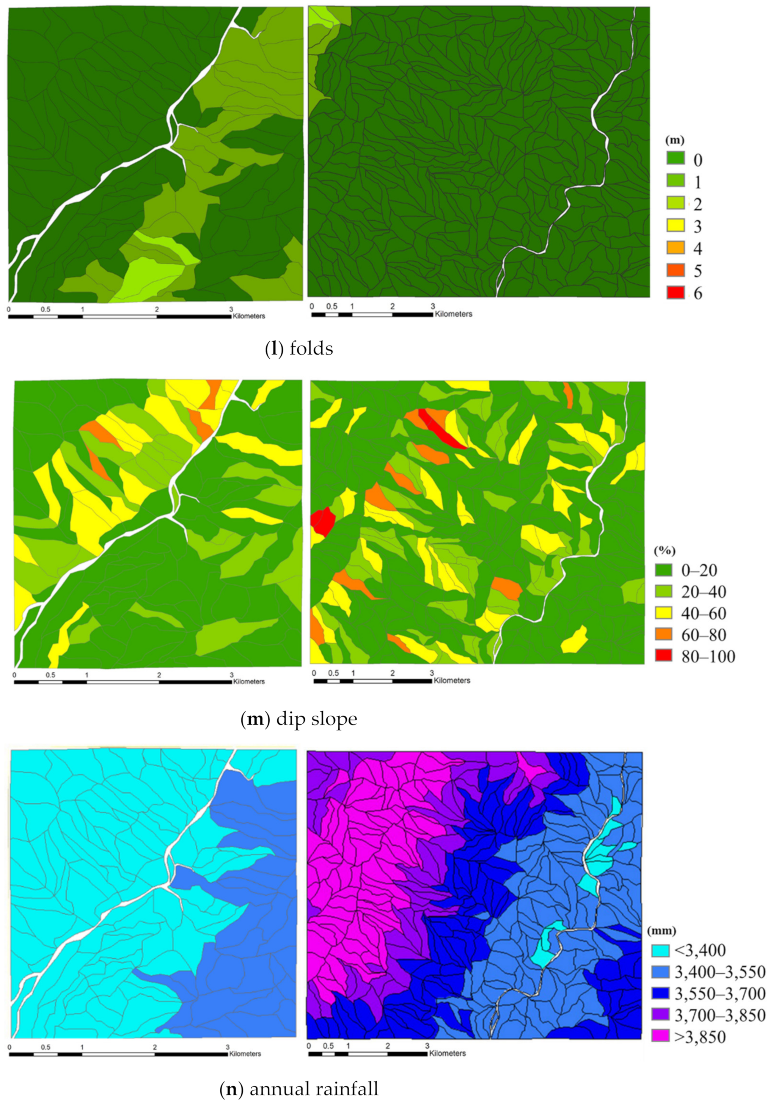
- Folds
- Dip Slopes
2.2.4. Driving Category (Rainfall)
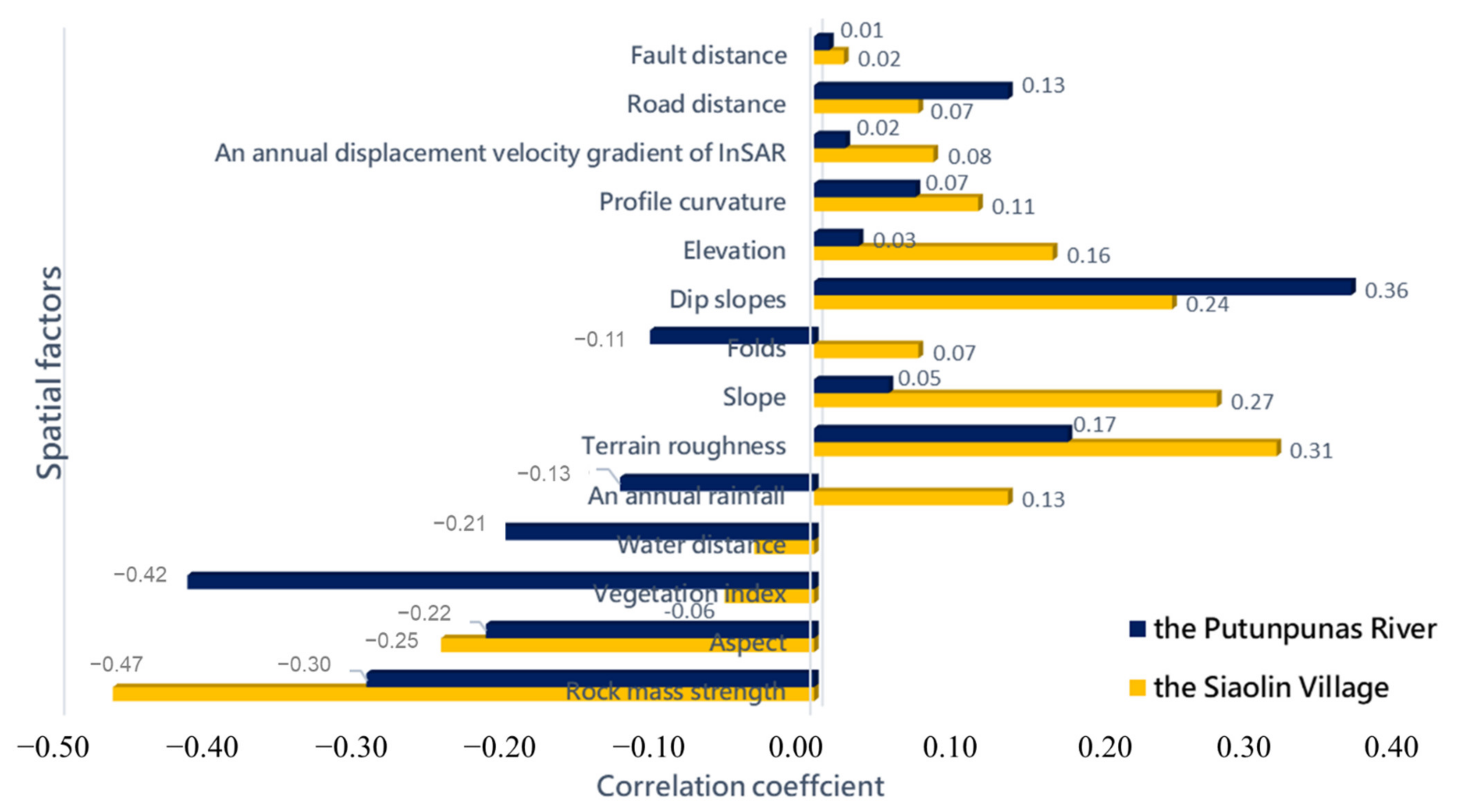
2.3. Correlation between Spatial Factors and Slope Landslides
2.4. Use of Machine Learning Methods
- Naive Bayes
- DT
- Random forest
- AdaBoost
- XGBoost
3. Results
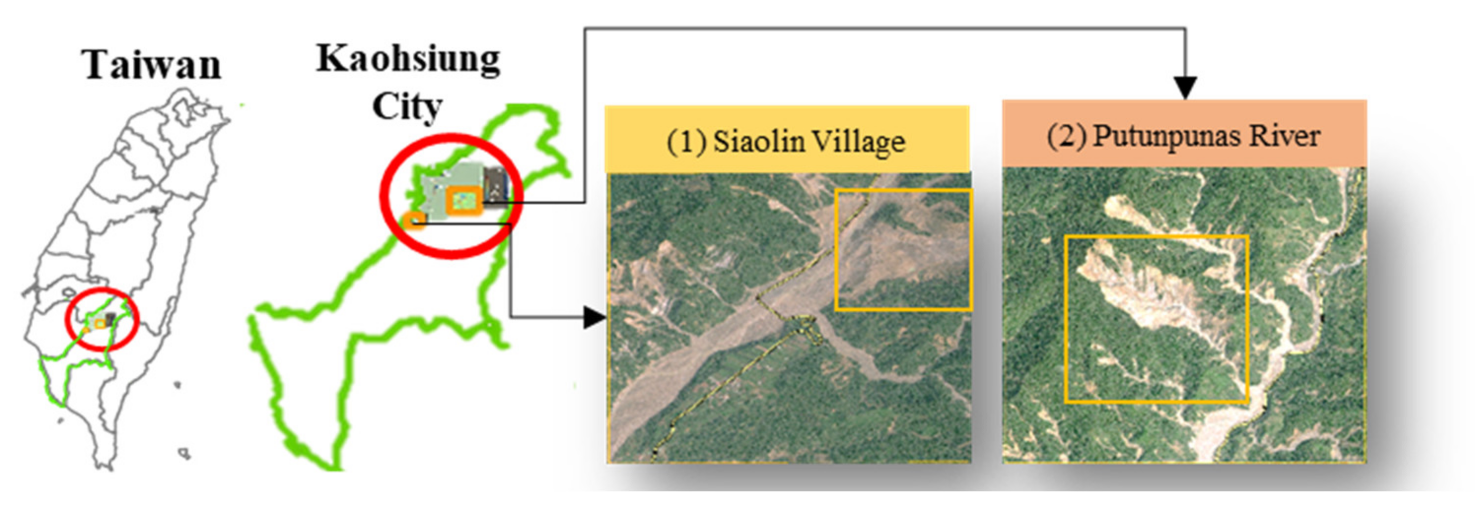
3.1. Study Areas
3.2. Significance Test of Spatial Factors
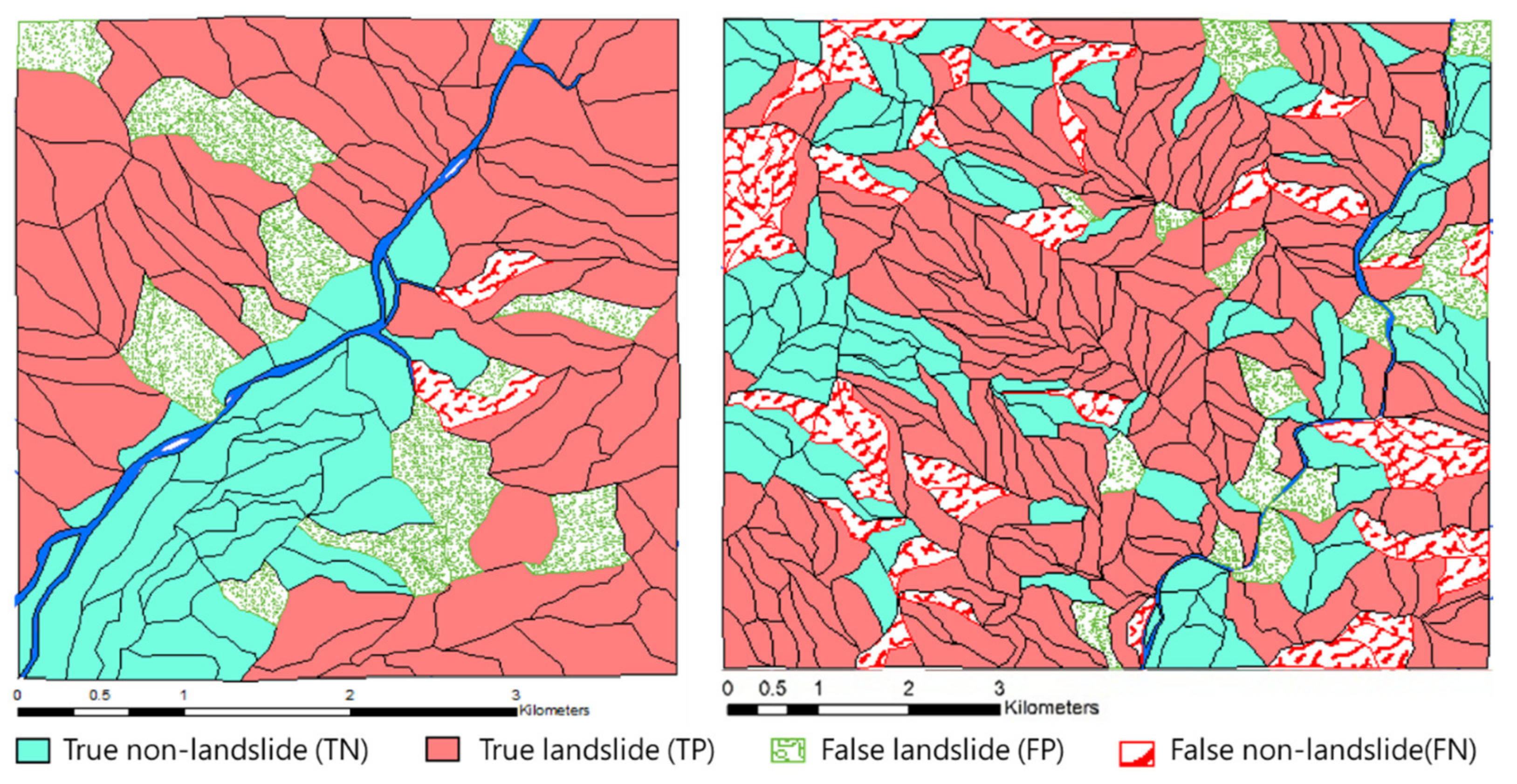
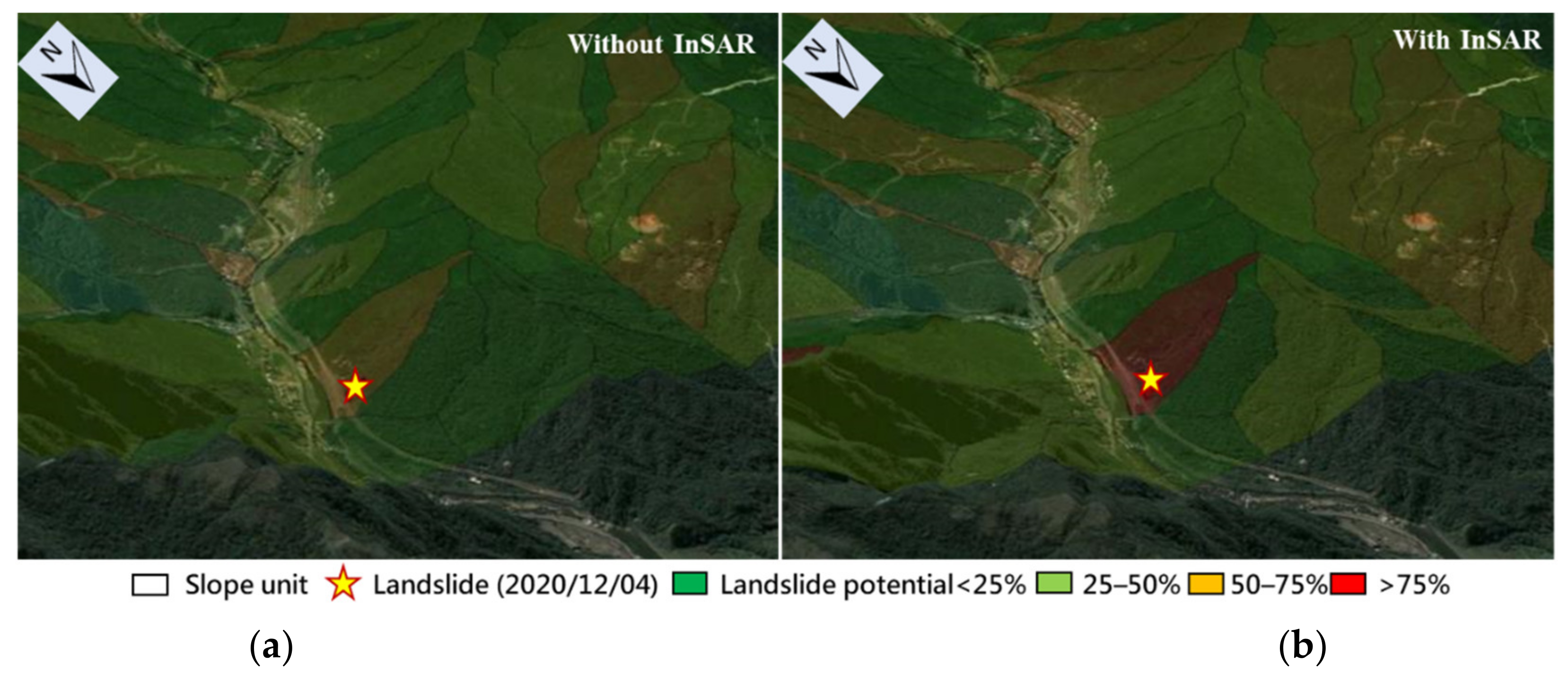
3.3. ML Prediction and Verification
4. Discussion
5. Conclusions
Author Contributions
Funding
Institutional Review Board Statement
Informed Consent Statement
Data Availability Statement
Acknowledgments
Conflicts of Interest
References
- Lin, S.C.; Ke, M.C.; Lo, C.M. Evolution of landslide hotspots in Taiwan. Landslides 2017, 14, 1491–1501. [Google Scholar] [CrossRef]
- Ma, Z.; Mei, G.; Piccialli, F. Machine learning for landslides prevention: A survey. Neural Comput. Appl. 2020, 1–27. [Google Scholar] [CrossRef]
- Benoit, L.; Briole, P.; Martin, O.; Thom, C.; Malet, J.P.; Ulrich, P. Monitoring landslide displacements with the Geocube wireless network of low-cost GPS. Eng. Geol. 2015, 195, 111–121. [Google Scholar] [CrossRef]
- Wang, G. GPS Landslide Monitoring: Single Base vs. Network Solutions—A case study based on the Puerto Rico and Virgin Islands Permanent GPS Network. J. Geod. Sci. 2011, 1, 191–203. [Google Scholar] [CrossRef] [Green Version]
- Ciuffi, P.; Bayer, B.; Berti, M.; Franceschini, S.; Simoni, A. Deformation Detection in Cyclic Landslides Prior to Their Reactivation Using Two-Pass Satellite Interferometry. Appl. Sci. 2021, 11, 3156. [Google Scholar] [CrossRef]
- Guzzetti, F.; Mondini, A.C.; Cardinali, M.; Fiorucci, F.; Santangelo, M.; Chang, K.T. Landslide inventory maps: New tools for an old problem. Earth-Sci. Rev. 2012, 112, 42–66. [Google Scholar] [CrossRef] [Green Version]
- Dabiri, Z.; Hölbling, D.; Abad, L.; Helgason, J.K.; Sæmundsson, Þ.; Tiede, D. Assessment of Landslide-Induced Geomorphological Changes in Hítardalur Valley, Iceland, Using Sentinel-1 and Sentinel-2 Data. Appl. Sci. 2020, 10, 5848. [Google Scholar] [CrossRef]
- Ramirez, R.; Lee, S.R.; Kwon, T.H. Long-Term Remote Monitoring of Ground Deformation Using Sentinel-1 Interferometric Synthetic Aperture Radar (InSAR): Applications and Insights into Geotechnical Engineering Practices. Appl. Sci. 2020, 10, 7447. [Google Scholar] [CrossRef]
- Ventisette, C.D.; Righini, G.; Moretti, S.; Casagli, N. Multitemporal landslides inventory map updating using spaceborne SAR analysis. Int. J. Appl. Earth Obs. Geoinf. 2014, 30, 238–246. [Google Scholar] [CrossRef] [Green Version]
- Shirani, K.; Pasandi, M. Detecting and monitoring of landslides using persistent scattering synthetic aperture radar interferometry. Environ. Earth Sci. 2019, 78, 42. [Google Scholar] [CrossRef]
- Carlà, T.; Intrieri, E.; Raspini, F.; Bardi, F.; Farina, P.; Ferretti, A.; Colombo, D.; Novali, F.; Casagli, N. Perspectives on the prediction of catastrophic slope failures from satellite InSAR. Sci. Rep. 2019, 9, 14137. [Google Scholar] [CrossRef] [Green Version]
- Utomo, D.; Chen, S.F.; Hsiung, P.A. Landslide Prediction with Model Switching. Appl. Sci. 2019, 9, 1839. [Google Scholar] [CrossRef] [Green Version]
- Chen, H.E.; Chiu, Y.Y.; Tsai, T.L.; Yang, J.C. Effect of Rainfall, Runoff and Infiltration Processes on the Stability of Footslopes. Water 2020, 12, 1229. [Google Scholar] [CrossRef]
- Bui, D.T.; Tuan, T.A.; Klempe, H.; Pradhan, B.; Revhaug, I. Spatial prediction models for shallow landslide hazards: A comparative assessment of the efficacy of support vector machines, artificial neural networks, kernel logistic regression, and logistic model tree. Landslides 2016, 13, 361–378. [Google Scholar]
- Al-Najjar, H.A.H.; Pradhan, B. Spatial landslide susceptibility assessment using machine learning techniques assisted by additional data created with generative adversarial networks. Geosci. Front. 2021, 12, 625–637. [Google Scholar] [CrossRef]
- Nsengiyumva, J.B.; Valentino, R. Predicting landslide susceptibility and risks using GIS-based machine learning simulations, case of upper Nyabarongo catchment. Geomat. Nat. Hazards Risk 2020, 11, 1250–1277. [Google Scholar] [CrossRef]
- Nhu, V.H.; Zandi, D.; Shahabi, H.; Chapi, K.; Shirzadi, A.; Al-Ansari, N.; Singh, S.K.; Dou, J.; Nguyen, H. Comparison of Support Vector Machine, Bayesian Logistic Regression, and Alternating Decision Tree Algorithms for Shallow Landslide Susceptibility Mapping along a Mountainous Road in the West of Iran. Appl. Sci. 2020, 10, 5047. [Google Scholar] [CrossRef]
- Shha, S.; Saha, A.; Hembram, T.K.; Pradhan, B.; Alamri, A.M. Evaluating the Performance of Individual and Novel Ensemble of Machine Learning and Statistical Models for Landslide Susceptibility Assessment at Rudraprayag District of Garhwal Himalaya. Appl. Sci. 2020, 10, 3772. [Google Scholar] [CrossRef]
- Lin, Y.T.; Yen, H.Y.; Chang, N.H.; Lin, H.M.; Han, J.Y.; Yang, K.H.; Chen, C.S.; Zheng, H.K.; Hsu, J.Y. Prediction of Landslides Using Machine Learning Techniques Based on Spatio-temporal Factors and InSAR Data. J. Chin. Inst. Civ. Hydraul. Eng. 2021, 33, 93–104. [Google Scholar]
- Yu, L.; Cao, Y.; Zhou, C.; Wang, Y.; Huo, Z. Landslide Susceptibility Mapping Combining Information Gain Ratio and Support Vector Machines: A Case Study fromWushan Segment in the Three Gorges Reservoir Area, China. Appl. Sci. 2019, 9, 4756. [Google Scholar] [CrossRef] [Green Version]
- Hu, X.; Zhang, H.; Mei, H.; Xiao, D.; Li, Y.; Li, M. Landslide Susceptibility Mapping Using the Stacking Ensemble Machine Learning Method in Lushui, Southwest China. Appl. Sci. 2020, 10, 4016. [Google Scholar] [CrossRef]
- Chen, W.; Shahabi, H.; Zhang, S.; Khosravi, K.; Shirzadi, A.; Chapi, K.; Pham, B.T.; Zhang, T.; Zhang, L.; Chai, H.; et al. Landslide Susceptibility Modeling Based on GIS and Novel Bagging-Based Kernel Logistic Regression. Appl. Sci. 2018, 8, 2540. [Google Scholar] [CrossRef] [Green Version]
- Chen, W.; Sun, Z.; Han, J. Landslide Susceptibility Modeling Using Integrated Ensemble Weights of Evidence with Logistic Regression and Random Forest Models. Appl. Sci. 2019, 9, 171. [Google Scholar] [CrossRef] [Green Version]
- Wang, H.; Zhang, L.; Yin, K.; Luo, H.; Li, J. Landslide identification using machine learning. Geosci. Front. 2021, 12, 351–364. [Google Scholar] [CrossRef]
- Truong, X.L.; Mitamura, M.; Kono, Y.; Raghavan, V.; Yonezawa, G.; Truong, X.Q.; Do, T.H.; Bui, D.T.; Lee, S. Enhancing Prediction Performance of Landslide Susceptibility Model Using Hybrid Machine Learning Approach of Bagging Ensemble and Logistic Model Tree. Appl. Sci. 2018, 8, 1046. [Google Scholar] [CrossRef] [Green Version]
- Pourghasemi, H.R.; Rahmati, O. Prediction of the landslide susceptibility: Which algorithm, which precision? Catena 2018, 162, 177–192. [Google Scholar] [CrossRef]
- Korup, O.; Stolle, A. Landslide prediction from machine learning. Geol. Today 2014, 30, 26–33. [Google Scholar] [CrossRef]
- Niu, X.; Ma, J.; Wang, Y.; Zhang, J.; Chen, H.; Tang, H. A Novel Decomposition-Ensemble Learning Model Based on Ensemble Empirical Mode Decomposition and Recurrent Neural Network for Landslide Displacement Prediction. Appl. Sci. 2021, 11, 4684. [Google Scholar] [CrossRef]
- Samia, J.; Temme, A.; Bregt, A.; Wallinga, J.; Guzzetti, F.; Ardizzone, F.; Rossi, M. Do landslides follow landslides? Insights in path dependency from a multi-temporal landslide inventory. Landslides 2017, 14, 547–558. [Google Scholar] [CrossRef] [Green Version]
- Wu, J.; Zeng, W.; Yan, F. Hierarchical Temporal Memory method for time-series-based anomaly detection. Neurocomputing 2018, 273, 535–546. [Google Scholar] [CrossRef]
- Xie, M.; Esaki, T.; Zhou, G. GIS-Based Probabilistic Mapping of Landslide Hazard Using a Three-Dimensional Deterministic Model. Nat. Hazards 2004, 33, 265–282. [Google Scholar] [CrossRef]
- Franklin, J.A. Safety and economy in tunneling. In Proceedings of the 10th Canadian Rock Mechanics Symposium, Kingston, ON, Canada, 2–4 September 1975; Volume 1, pp. 27–53. [Google Scholar]
- Rish, I. An empirical study of the naive Bayes classifier. In Proceedings of the IJCAI 2001 Workshop on Empirical Methods in Artificial Intelligence, Seattle, WA, USA, 4–6 August 2001; Volume 3, pp. 41–46. [Google Scholar]
- Safavian, S.R.; Landgrebe, D. A survey of decision tree classifier methodology. IEEE Trans. Syst. Man Cybern. 1991, 21, 660–674. [Google Scholar] [CrossRef] [Green Version]
- Ho, T.K. Random decision forests. In Proceedings of the 3rd International Conference on Document Analysis and Recognition, Montreal, QC, Canada, 14–16 August 1995; Volume 1, pp. 278–282. [Google Scholar]
- Freund, Y.; Schapire, R.E. A decision-theoretic generalization of on-line learning and an application to boosting. J. Comput. Syst. Sci. 1997, 55, 119–139. [Google Scholar] [CrossRef] [Green Version]
- Friedman, J.H. Stochastic gradient boosting. Comput. Stat. Data Anal. 2002, 38, 367–378. [Google Scholar] [CrossRef]


| Spatial Factor | Siaolin Village | Putunpunas River | ||
|---|---|---|---|---|
| Correlation Coefficient | p-Value | Correlation Coefficient | p-Value | |
| Rock mass strength | −0.47 | 1.00 | −0.30 | 1.00 |
| Aspect | −0.25 | 1.00 | −0.22 | 1.00 |
| Vegetation index | −0.06 | 0.49 | −0.42 | 1.00 |
| Water distance | −0.04 | 0.37 | −0.21 | 1.00 |
| Annual rainfall | 0.13 | 0.85 | −0.13 | 0.98 |
| Terrain roughness | 0.31 | 1.00 | 0.17 | 1.00 |
| Slope | 0.27 | 1.00 | 0.05 | 0.66 |
| Folds | 0.07 | 0.57 | −0.11 | 0.95 |
| Dip slopes | 0.24 | 0.99 | 0.36 | 1.00 |
| Elevation | 0.16 | 0.93 | 0.03 | 0.37 |
| Profile curvature | 0.11 | 0.81 | 0.07 | 0.78 |
| Annual displacement velocity gradient of InSAR | 0.08 | 0.62 | 0.02 | 0.29 |
| Road distance | 0.07 | 0.59 | 0.13 | 0.98 |
| Fault distance | 0.02 | 0.28 | 0.01 | 0.23 |
| ML | Parameters | Values |
|---|---|---|
| Naive Bayes | Smoothing | 10−9 |
| DT | Criterion | Gini |
| The maximum of depth | 20 | |
| The minimum of samples split | 10 | |
| The minimum of samples leaf | 5 | |
| Random Forest | Criterion | Gini |
| The maximum of depth | 20 | |
| The minimum of samples split | 2 | |
| The minimum of samples leaf | 5 | |
| The number of estimators | 100 | |
| AdaBoost | Criterion | Gini |
| The maximum of depth | 20 | |
| The minimum of samples split | 2 | |
| The minimum of samples leaf | 5 | |
| The number of estimators | 10 | |
| Algorithm | SAMME | |
| Learning rate | 0.1 | |
| XGBoost | The maximum of depth | 5 |
| The number of estimators | 1000 | |
| Learning rate | 0.1 | |
| The minimum of child weight | 1 | |
| Gamma number | 0 | |
| Subsample number | 0.8 | |
| Colsample bytree | 0.8 | |
| Objective binary | Logistic | |
| nthread | 4 |
| ML | Siaolin Village | Putunpunas River | ||
|---|---|---|---|---|
| With InSAR (%) | Without InSAR (%) | With InSAR (%) | Without InSAR (%) | |
| Naive Bayes | 70.93 | 70.85 | 68.19 | 68.19 |
| DT | 68.02 | 62.02 | 75.45 | 75.07 |
| Random Forest | 82.95 | 79.84 | 80.52 | 78.79 |
| AdaBoost | 78.49 | 77.52 | 75.64 | 75.64 |
| XGBoost | 79.31 | 75.97 | 78.80 | 75.80 |
| Predictied | Lanslide | Nonlanslide | Average | |
|---|---|---|---|---|
| Actual | ||||
| Lanslide | 74 (TP) | 2 (FN) | - | |
| Nonlanslide | 20 (FP) | 33 (TN) | - | |
| Correct rate (%) | 78.72 | 94.30 | 82.95 | |
| Predictied | Lanslide | Nonlanslide | Average | |
|---|---|---|---|---|
| Actual | ||||
| Lanslide | 191 (TP) | 46 (FN) | - | |
| Nonlanslide | 22 (FP) | 90 (TN) | - | |
| Correct rate (%) | 89.67 | 66.18 | 80.52 | |
Publisher’s Note: MDPI stays neutral with regard to jurisdictional claims in published maps and institutional affiliations. |
© 2021 by the authors. Licensee MDPI, Basel, Switzerland. This article is an open access article distributed under the terms and conditions of the Creative Commons Attribution (CC BY) license (https://creativecommons.org/licenses/by/4.0/).
Share and Cite
Lin, Y.-T.; Chen, Y.-K.; Yang, K.-H.; Chen, C.-S.; Han, J.-Y. Integrating InSAR Observables and Multiple Geological Factors for Landslide Susceptibility Assessment. Appl. Sci. 2021, 11, 7289. https://doi.org/10.3390/app11167289
Lin Y-T, Chen Y-K, Yang K-H, Chen C-S, Han J-Y. Integrating InSAR Observables and Multiple Geological Factors for Landslide Susceptibility Assessment. Applied Sciences. 2021; 11(16):7289. https://doi.org/10.3390/app11167289
Chicago/Turabian StyleLin, Yan-Ting, Yi-Keng Chen, Kuo-Hsin Yang, Chuin-Shan Chen, and Jen-Yu Han. 2021. "Integrating InSAR Observables and Multiple Geological Factors for Landslide Susceptibility Assessment" Applied Sciences 11, no. 16: 7289. https://doi.org/10.3390/app11167289