Article

Context-Based Structure Mining Methodology for Static Object Re-Identification in Broadcast Content

by
Krishna Kumar Thirukokaranam Chandrasekar
* and
Steven Verstockt
IDLab, Ghent University—imec, 9052 Ghent, Belgium
*
Author to whom correspondence should be addressed.
Appl. Sci. 2021, 11(16), 7266; https://doi.org/10.3390/app11167266
Submission received: 27 June 2021 / Revised: 3 August 2021 / Accepted: 4 August 2021 / Published: 6 August 2021
(This article belongs to the Special Issue Artificial Intelligence for Multimedia Signal Processing)

Abstract

:
Technological advancement, in addition to the pandemic, has given rise to an explosive increase in the consumption and creation of multimedia content worldwide. This has motivated people to enrich and publish their content in a way that enhances the experience of the user. In this paper, we propose a context-based structure mining pipeline that not only attempts to enrich the content, but also simultaneously splits it into shots and logical story units (LSU). Subsequently, this paper extends the structure mining pipeline to re-ID objects in broadcast videos such as SOAPs. We hypothesise the object re-ID problem of SOAP-type content to be equivalent to the identification of reoccurring contexts, since these contexts normally have a unique spatio-temporal similarity within the content structure. By implementing pre-trained models for object and place detection, the pipeline was evaluated using metrics for shot and scene detection on benchmark datasets, such as RAI. The object re-ID methodology was also evaluated on 20 randomly selected episodes from broadcast SOAP shows New Girl and Friends. We demonstrate, quantitatively, that the pipeline outperforms existing state-of-the-art methods for shot boundary detection, scene detection, and re-identification tasks.

1. Introduction

Due to advances in storage and digital media technology, videos have become the main source of visual information. The recording and accumulation of a large number of videos has also become very easy, and many popular websites, including YouTube, Yahoo Video, Facebook, Flickr, and Instagram, allow users to share and upload video content globally. Today, we have arrived at the point where the volume of video that arrives on the internet increases exponentially on a daily basis. Apart from this, there are very many broadcast channels with enormous amounts of video content—shot and stored every second. With such large collections of videos, it is very difficult to locate the appropriate video files and extract information from them effectively. Moreover, with such a vast quantity of data, even the suggestion list expands tremendously; thus, it is even more difficult to make an efficient and informed decision. Large file sizes, the temporal nature of the content, and the lack of proper indexing methods to leverage non-textual features, creates difficulty in cataloguing and retrieving videos efficiently [1]. To address these challenges, efforts are being made—in every direction—to bridge the gap between low-level binary video representations and high-level text-based video descriptions (e.g., video categories, types or genre) [2,3,4,5,6,7]. Due to the absence of structured intermediate representations, powerful video processing methodologies which can utilise scene, object, person, or event information do not yet exist. In this paper, we address this problem by proposing a framework involving an improved semantic content mining approach, which obtains frame-level location and object information across the video. The proposed architecture extracts semantic tags such as objects, actions and locations from the videos, using them not only to obtain scene/shot boundaries, but also to re-ID objects from the video.
Since this paper deals with several video features/aspects, it is important to clearly state the definitions for the various structures and components of a video as used in this paper. Any video can essentially be broken down into several units. First, a video is a collection of successive images; specific frames shown at a particular speed. Each frame is one of the many still images that make up the video. Next, a group of uninterrupted and coherent frames constitute a shot. Every frame belongs to a shot, which lasts for a minimum of 1 s and is based on the frame rate of the broadcast video (which can be anywhere between 20 to 60 frames per second). Enriching every frame of a video would be computationally expensive and practically inefficient. Thus, we find it logical to consider a shot as the fundamental unit of the video. Based upon these shots, the entire video can be iteratively enriched with data, such as scene types, actions and events.
Humans, on the other hand, tend to remember specific events or scenarios from a video that they view during a video-retrieval process. Such an event could be a dialogue, an action scene, or any series of shots unified by location or a dramatic incident [8]. Therefore, it is events themselves which should be treated as an elementary retrieval unit in future advanced video retrieval systems. Various terms denoting temporal video segments on a level above shots, but below sequences, appear in the literature [9]. These include scenes, logical units, logical story units, and topic units. The flow diagram on Figure 1 shows how this space could be well-defined [10]. A logical story unit (LSU) could thus be a scene or a topic unit, depending on the type of content. Our proposed pipeline can automatically segment videos into logical story units.
Researchers often address semantic mining and structure mining problems separately, because they were historically applied to different domains. However, during the last decade, image recognition algorithms have improved exponentially, and deep learning models, together with GPU/TPU computational hardware, allow very accurate real-time detectors to be trained and served. This has paved the way to complex pipelines that can be defined and reused across multiple domains. We have made use of these technological advancements in defining a versatile semantic extraction pipeline that proves to address multiple video analytic problems simultaneously. In summary, the main contributions of this paper can be listed as follows:
  • We propose a flexible pipeline that can derive high-level features from detection algorithms and semantically enrich a video by performing automatic video structure mining. This pipeline consolidates the frame-level place and object tags using time-efficient deep neural networks in such a way that it could be used for further enrichment tasks, such as re-ID.
  • Within the pipeline, we have implemented a novel boundary-detection algorithm to cluster the temporally coherent, semantically closer segments into shots and LSUs.
  • We also propose a novel multi-object re-ID algorithm-based on context similarity in SOAP and broadcast content to generate object timelines.
The remainder of this paper is organised as follows. Section 2 reviews related work. Subsequently, Section 3 presents our methodology, which explains, in detail, the algorithms used for semantic extraction, boundary prediction and object re-ID. The experimental set up and model selection are presented in Section 4. Section 5 discusses the results, while Section 6 concludes this paper and discusses the future work.

2. Related Work

This work elaborates the role of semantics in video analysis tasks such as video structure mining and re-ID. Spatial semantics includes the objects and persons in, as well as the location of, a frame. Temporal semantics includes actions, events, and their interactions across the video. For a system to understand a video, therefore, the system requires the ability to automatically comprehend such spatio-temporal relationships. In the following subsections, we discuss various approaches for semantic extraction, LSU/shot boundary detection and re-ID methodologies.

2.1. Semantic Extraction

2.1.1. Image Classification and Localization

Image classification and object recognition tasks have been investigated for a long time. Yet, for much of this period, there were no suitable general solutions available. This was mainly attributed to the quality of training data and accessible computational hardware. Moreover, the classification accuracy when using a smaller, rather than a larger, number of classes was observed to be greater [11]. However, performance in image-classification tasks has been exponentially improved in open competitions, such as the Large Scale Visual Recognition Challenge (ILSVRC) and MIT-Places-365. These competitions encouraged the development of region proposal network (RPN)-based deep neural networks, including AlexNet, GoogleNet and Vision Geometry Group (VGG). These networks have revolutionised image classification and have opened doors, in all directions, for classification and annotation. We use the VGG-16 network trained on MIT-Places-365 for obtaining the place/location of a frame, because it is very generalised and the architecture could be reused for further tasks, including the Dense Captioning of a frame that also has VGG-16 as its base architecture.
In addition to classification tasks, the success of the above-mentioned challenges has also fuelled research on localisation and detection tasks. Speed and accuracy have been the major areas of focus and, based on these, there are two major types of object detection models: (1) region-based convolution models, such as R-CNN and Faster RCNN, that split the image into a number of sub-images, and (2) convolution models, such as Single Shot Detector (SSD) and You Only Look Once (YOLO), that detect objects in a single run [12]. Even though the Faster RCNN have slightly higher accuracy, the latest version of YOLO (YOLOv3 [12]) detects objects up to 20 times faster while retaining similar/acceptable accuracy. Thus, our pipeline has a pre-trained YOLOv3 model that has been used for detecting objects and persons in a frame.

2.1.2. Video Annotation

There has also been research pertaining to video annotation. [13] proposed an event-based approach to create text annotations, which infers high-level textual descriptions of events. This method does not take into account the temporal flow or correlations between different events in the same video. Thus, the approach does not have the ability to interact or fuse multiple events into scenes or activities. As explained in the previous section, it is important to search for and retrieve continuous blocks of video, often referred to as scenes or story units.
Stanislav Protasov et al. [14] proposed a pipeline with keyframe-based annotation of scene descriptions, while [15] proposed a sentence-generation pipeline which provides descriptions for keyframes based on the semantic information. Even though the techniques produced acceptable results, the annotations still lacked information and faced information losses. Torralba et al. [16], on the other hand, proposed a solution for semantic video annotation that consists of per-frame annotations of scene tags. The per-frame annotations are computationally expensive and often redundant. Therefore, we incorporated a pipeline that takes into account the drawbacks of these previous methodologies. The pipeline obtains all possible spatial information, ranging from the location to objects and persons, in the form of textual descriptions for every nth frame of the video. This n depends on the frame rate of the video and is adjusted so that textual descriptions are obtained for a minimum of 4 frames per second.

2.2. Boundary Detection

Shot and scene detection is one of the long-studied problems in video structure mining. There have been a lot of different approaches based on the different features used and the different clustering methods available. In this subsection we discuss the latest approaches for shot and LSU detection.
In the existing works for shot boundary detection, there a prevailing and striking pattern of similarities. We have come to the conclusion that boundary detection is performed by calculating or learning the deviation of features over adjacent frames. Widely used features include RGB, HSV, or LUV colour histograms [17], background similarity [4], motion features [18], edge ratio change and SIFT [19], and spectral features. Ref. [17] uses a spectral clustering algorithm to cluster shots, while [18] proposes a new adaptive scene-segmentation algorithm that uses the adaptive weighting of colour and motion similarity to distinguish between two shots. They also propose an improved overlapping-links scheme to reduce shot grouping time. Recently, deep features, extracted using CNN, were employed to obtain significant state-of-the-art results [20]. This team used an end-to-end trainable CNN model that was trained using a cross entropy loss to detect shot transitions. In this work, we employ frame-level object-, person- and location-type semantic descriptions as features to estimate shot boundaries.
For scene detection, Stanislav Protasov et al. [14] proposed a pipeline that utilises scene descriptions for keyframes of shots, while [15] proposed a pipeline that generates sentences or captions based on objects in a keyframe. The former utilises a scene transition graph to cluster similar shots to scenes, while the latter proposes to use Jaccard-similarity for obtaining similarity between shots. As per survey [21], the LSU-detection task is understood as a three-stage problem. In the first step, frames are grouped into shots. In the second step, location, person and object descriptions are consolidated to obtain shot-level descriptions. In the third stage, shot-level descriptions are used to cluster the shots into story units, using a similarity metric and assumptions about the film structure. For shot boundary detection, we have proposed and utilised the shot-detection algorithm defined in our methodology.

3. Methodology

Based on the motivations explained in Section 1, we propose a pipeline that utilises semantic descriptions and their co-occurrences across a video to address the fundamental video processing challenges pertaining to structure mining and object re-ID tasks. The proposed pipeline is shown in Figure 2. We follow a step-wise approach to explain the implementation of the pipeline:
  • Semantic Extraction
  • Structure Mining
  • Similarity Estimation
  • Object Re-Identification

3.1. Semantic Extraction: Recognizing Objects, Places and Their Relations

In order to work with the high-level semantic features, it is important to have thorough information regarding the composition of each frame (e.g., objects, persons, and places in the frame). Since broadcast videos do not carry that much frame-level semantic information, it is necessary for our pipeline to have a good model that can predict, with high accuracy, the objects and places in a frame. As seen in Figure 2, frame-level semantic extraction is a common step for all the tasks dealt with in the paper—from shot/LSU boundary prediction to object timeline generation.

Feature Extraction

We make use of low-level and mid-level visual information for predicting the high-level features that are necessary to determine the semantic composition of a logical story unit. In our approach we use object, person and location tags as high-level features for detecting the LSU boundaries. To obtain the object and person annotations, the latest version of the YOLO object detector [12], pre-trained on the COCO dataset [22], is used. COCO stands for Common Objects in Context. The dataset comprises of 1.5 million object instances covering 80 object classes. Along with the object detector, the place or the location of the scenes are predicted using the ResNet-50 CNN architecture, pretrained on the places-365 dataset [11]. This dataset contains more than 10 million images in total, comprising 400+ unique scene categories [23].

3.2. Structure Mining: Shot Boundary Detection

Once we extract the visual features of the video frames, we utilise them to estimate the similarity between frames. This, in turn, is used to predict the overall structure of the video as shown in Figure 3. Broadcast videos generally have a frame rate of 24 fps. We process every sixth frame of our video for computational advantage (4 frames/s). Furthermore, we cluster temporally similar frames to form shot and story units.
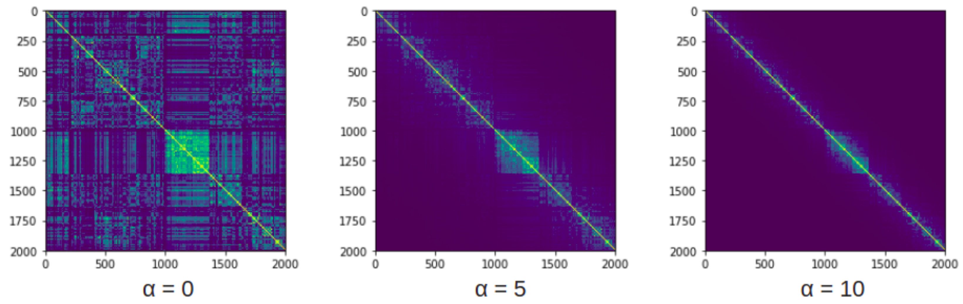
  • Spatio-Temporal Visual Similarity Modelling
In contrast to other approaches that use clustering for boundary detection, we construct a similarity matrix that jointly describes spatial similarity and temporal proximity. The generic element S i j defines the similarity between frames i and j, as shown in Equation (1).
S i j = e x p d 1 2 ( ψ ( x i ) , ψ ( x j ) ) + α · d 2 2 ( x i , x j ) 2 σ 2
where, ψ ( x i ) and ψ ( x j ) are the list of visual tags for the ith and jth frame, respectively. d 1 2 is the cosine distance between frame x i and x j , while d 2 2 is the normalised temporal distance between frame x i and frame x j . The parameter α tunes the relative importance of semantic similarity and temporal distance. The effect of alpha on the similarity matrix is shown in Figure 4.
As shown in Figure 4, the effect of applying increasing values of α to the similarity matrix is to raise the similarities of adjacent frames, thereby boosting the temporal correlations of frames in the neighbourhood. At the same time, too high values of α would lead to the boosting of the temporal correlation of very close neighbouring frames, thereby failing to capture gradual shot changes. The final boundaries are created between frames that do not belong to the same cluster. An experiment was conducted with the videos of the RAI dataset, where values from 1 to 10 were provided for α , and its effect was studied. We found that an α value of 5 performed well on average, for both gradual and sharp shot changes. Therefore, we use an α value of 5 for our shot boundary detection experiments, since it provides the right amount of local temporal similarity for the prediction of boundaries.
As seen in Equation (1), semantic composition-based frame-similarity estimation is composed of the following two sub parts:
  • Semantic similarity scoring scheme
  • Temporal model analysis

3.2.1. Semantic Similarity Scoring Scheme

We use the cosine similarity principle to measure inter-frame similarity; that is, we measure the cosine angle between the two frame vectors of interest. The cosine similarity between the ith and the jth frame is calculated by taking the normalised dot product as follows:
s i m ( x i , x j ) = | | ψ ( x i ) | | · | | ψ ( x j ) | |
where, ψ ( x i ) is the normalised vector based on the list of visual tags for frame x i . This results in a spatial similarity matrix. The similarity measure is converted into a distance measure based on the following Equation:
d 1 2 ( ψ ( x i ) , ψ ( x j ) ) = 1 s i m ( x i , x j )
An example of utilising the spatial similarity matrix to retrieve the top four similar frames from a video is shown in Figure 5.

3.2.2. Temporal Model Analysis

As per Equation (1) the temporal proximity is modelled using d 2 2 , which is the normalised temporal distance between frames x i and x j . The normalised temporal distance can be defined by Equation (4)
d 2 2 ( x i , x j ) = | f i f j | l
where f i and f j are the index of frame x i and x j , respectively, and l is the total number of frames in the video.

3.2.3. Boundary Prediction

Based on Equation (1), the lower the value of S i j , the more dissimilar frames x i and x j are. Thus, we calculate the shot boundary by thresholding S i j . In our experiments, 0.4 was used as the threshold value. The entire shot boundary detection algorithm is shown in Algorithm 1.
Algorithm 1: Shot boundary detection
Applsci 11 07266 i001

3.3. Similarity Estimation: Context Based Logical Story Unit Detection

Based on our experiments, we have deduced that normal broadcast content, such as a SOAP episode or the news, often make use of multiple angles pertaining to the same story unit.In more than 90% of the cases, these angles recur multiple times throughout the video. Therefore, as shown in Figure 6, the context-based similarity estimation begins with shot detection. Progressing from these estimated shot boundaries, frame-level semantic descriptions are merged as follows:
L i j = w 1 ( p l a c e _ s i m ) + w 2 ( o b j _ s i m ) w 1 + w 2
where w 1 and w 2 are the weights for place and object descriptions. In our experiments, we have given more importance to place descriptions than to object descriptions, mainly because the state-of-the-art object detection models do not have the ability to predict all the objects in a frame. Moreover, the pre-trained place-detection model has the ability to capture the overall context of the shot location, and therefore has been deemed more important. Thus we have maintained w 1 and w 2 as 2 and 1, respectively, in all our experiments.
The shot-level similarity measure is calculated based on the joint similarity estimated using Equation (5). An example of the similarity matrix of a video from RAI is shown in Figure 7. The final similarity matrix is used along with the re-identification algorithm to generate object timelines.

3.4. Object Re-Identification

We propose an algorithm that formulates unique object IDs using LSUs and frame-level object detections, such that re-occurring objects are provided with the same ID. The algorithm we propose is based on the following hypothesis:
Hypothesis 1.
If two shots S a and S b are similar, then the objects present in S a and S b are also similar.

3.4.1. Explanation

Multimedia broadcast content, such as SOAP, news, or talk shows, often reuse locations that conserve the objects that they contain. Then, based on the above hypothesis, the objects are the same if they are present in the same location. For example, in Figure 8, Image 1 is frame 26070 of the video and image 2 is frame 27604. Although they are approximately 1500 frames apart, they both pertain to the same location, and thus the objects in them are the same. An important point to note is that the hypothesis holds only for stationary/static objects; if there are dynamic objects present in the shots (e.g., persons) the hypothesis will fail. Our approach focuses only on static object re-identification—thus, the current paper will only address problems of this kind.
Based on the number of occurrences of a same class object in the same frame, the re-ID algorithm is composed of two sub-parts:
  • Single instance
  • Multiple instance

3.4.2. Single Instance

If there is just a single occurrence of the object in every frame it appears in throughout the video, then by Hypothesis 1, the i d for object O at frame n is given by Equation (6) as follows:
O i d n = i d = 1 , n = 0 O i d a , S a n > t h r e s h o l d , i d + 1 , S a n < t h r e s h o l d , where   ( a = 1 : n 1 )
where in O i d n is the object i d at frame n, and S a n is the context-similarity measure between the frame a and n as calculated in Equation (5).

3.4.3. Multiple Instance

If there are multiple occurrences of the object, we propose a graph-based approach to correctly localise the object in the frame. An example of this problem is shown in Figure 8. In such cases, where multiple objects of the same class exist, it is not only important to know whether shot/LSU of the frames are similar, but also to know the spatial position/location of the object in the frame, so that the object can be re-IDed correctly.
Therefore, based on the bounding box co-ordinates of the detected objects, a location graph is estimated using spatial distances between the objects, as shown in Figure 9. The idea here is to generate and compare the graphs such that the IDs of the objects can be matched.
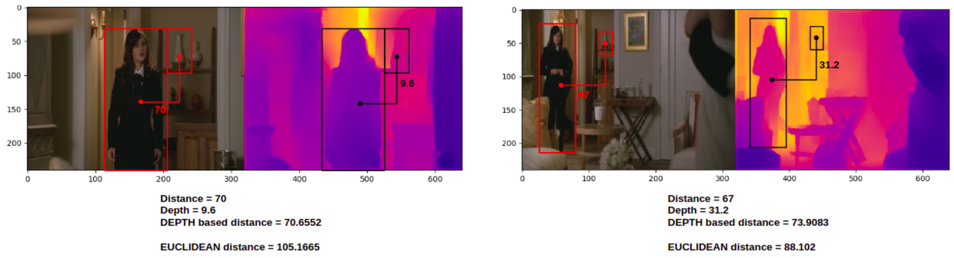
  • Spatial Distance Estimation
Although, the 2-D Euclidean distance measure works well between frames with similar angles across similar LSUs, there are cases where the angle and zoom changes across similar LSUs. The topological information contained within the frame is also lost, making it impossible to obtain a realistic distance estimation. To compensate for the topological information, we propose to use depth maps, in combination with the location graph, to estimate a more realistic spatial distance between the objects in a frame. To obtain depth information, we use Dense Depth [24], pre-trained on NYU Depth V2 dataset [25]. The estimated depth is used as a third dimension, and thereby the Euclidean measure is re-calculated as shown in Figure 10.
Let x and y be the centre points of the objects O x and O y , respectively, in a frame. Then the distance between them is given by:
d i s t a n c e = | x y |
The estimated depth has a range of values that are clipped between 10 and 1000, where 10 is the closest and 1000 is the farthest. If the depth values at points x and y can be represented as δ ( x ) and δ ( y ) , the depth between the objects can be estimated by:
d e p t h = | δ ( x ) δ ( y ) |
Finally, from Equations (7) and (8), the actual distance between the objects can be calculated as follows:
D x y = ( d i s t a n c e ) 2 + ( d e p t h ) 2
  • Spatial Location Graph
For every frame with multiple instance objects, the spatial location graph is estimated based upon the pairwise distance between the objects in the frame, using Equation (9). Let G i ( O , D ) and G j ( O , D ) be the graphs with objects as nodes and their distances as edges for two similar frames i and j. The objects in frame j are matched with the objects in i, based on comparing the distances between the objects in j and i such that the difference between the distances is always minimal. For instance, if frame i has 4 objects, O i 1 , O i 2 , O i 3 , O i 4 , of which O i 1 and O i 2 belong to the same class, and D i 12 , D i 13 denotes the distance between objects, then to re-identify objects O 1 in frame j, the sub-graph distances of G i [ O 1 ] and G i [ O 2 ] are compared with G i [ O 1 ] . O j 1 is deduced to be the same as the object in i for which the difference between distances is minimal. The overall object re-ID algorithm is shown in Algorithm 2 while the complete re-ID pipeline is shown in Figure 11.
Algorithm 2: Multi–object re–ID.
Applsci 11 07266 i002

4. Experiments

To provide a comprehensive overview of the strengths of the pipeline, it was separately evaluated on benchmark task-specific datasets. All the experiments were performed on a Linux Intel(R) Core(TM) i5-7440HQ CPU system with a RAM capacity of GB; the GPU was an NVidia GeForce 980 with 4 GB memory; and the operating system was Ubuntu version 16.04. The entire pipeline was implemented in Python 3.6 with the Pytorch deep learning library. The datasets and evaluation metrics used for evaluating our pipeline are explained in the following sections.

4.1. Dataset

In this work, a thorough, objective, and accurate performance evaluation has been carried out to evaluate the pipeline for shot boundary detection, LSU boundary detection and object re-ID.
To evaluate the proposed approach for shot and LSU boundary detection, we tested the pipeline on the benchmark RAI dataset. This dataset is a collection of ten challenging broadcasting videos from the Rai Scuola video archive, ranging from documentaries to talk shows constituted by both simple and complex transitions.
We evaluate our approach for object re-ID on randomly selected SOAP episodes. For fair evaluation, we chose to validate our approach on two different sets of SOAP broadcast content; namely, New Girl and Friends. We selected 10 episodes from Season 4 of New Girl and 10 episodes from Season 3 of Friends as our final dataset for object re-ID.

4.2. Evaluation Metrics

We evaluated the pipeline based on three tasks: (1) accuracy of the shot boundary detection; (2) accuracy of the LSU boundary detection; and (3) accuracy of the object re-ID algorithm.
For all the experiments, we use the precision, recall, and f1-score for the evaluation of our results. Precision, recall, and f1-score are computed based on the matched shots/LSU with the ground truth. Furthermore, the results were graphically visualised and analysed to promote insight.
The precision measure refers to the fraction of rightly predicted boundaries from total predictions, whereas recall measure denotes the fraction of boundaries rightly retrieved. If g r o u n d t r u t h refers to the list of ground-truth values and p r e d i c t i o n refers to the list of automatically predicted values, then precision and recall can be expressed as in Equation (10).
p r e c i s i o n = | g r o u n d t r u t h p r e d i c t i o n | | p r e d i c t i o n | r e c a l l = | g r o u n d t r u t h p r e d i c t i o n | | g r o u n d t r u t h |
F-score, on the other hand, combines precision and recall measures; it is the harmonic mean of the two. Traditional F s h o t can be defined as follows:
F s h o t = 2 · p r e c i s i o n · r e c a l l p r e c i s i o n + r e c a l l
As mentioned in earlier sections, the precision, recall, and f1 measure would not suffice to validate the accuracy of the LSU boundary detection algorithm. The reason for this is that humans and algorithms employ different ways of perceiving story units. Humans can relate changes in time and location to discontinuities in meaning, whereas an algorithm solely depends on visual dissimilarity to identify discontinuities. This semantic gap makes it impossible for algorithms to achieve fully correct detection results. Therefore, as suggested in [9], we use coverage and overflow metrics to measure how well our LSU boundary detection algorithm performs with respect to human labelled LSUs, using visual features. That is, in addition to the precision, recall, and f1 measures, we propose to use c o v e r a g e and o v e r f l o w measures to evaluate the number of frames that were correctly clustered together.
Coverage C measures the quantity of frames belonging to the same scene correctly grouped together, while Overflow O evaluates to what extent frames not belonging to the same scene are erroneously grouped together. Formally, given the set of automatically detected scenes s = [ s 1 , s 2 , , s m ], and the ground truth g = [ s 1 , s 2 , , s n ], where each element of s and g is a set of shot indexes, the coverage of scene s is proportional to the longest overlap between s i and g t :
c o v e r a g e = m a x i = 1 n # ( s i g t ) # ( g t )
o v e r f l o w = i = 1 m # ( s i / g t ) · m i n ( 1 , ( s i g t ) ) # ( g t 1 ) + # ( g t + 1 )
F s c e n e combines the coverage and overflow measures and is the harmonic mean of the two. For coverage, values closer to 1 indicate better performance, and for overflow, values closer to 0 indicate better; thus we use 1 o v e r f l o w for calculating F s c e n e :
F s c e n e = 2 · c o v e r a g e × ( 1 o v e r f l o w ) c o v e r a g e + ( 1 o v e r f l o w )
For the experiments pertaining to object re-ID, we make use of A c c u r a c y metrics. Accuracy is the most intuitive performance measure; it is simply the ratio of correctly predicted observations to total observations. In our scenario, the predicted observations are labelled as T r u e if they are correctly predicted, and F a l s e otherwise. Therefore, if the total number T r u e samples is denoted by T r u e , and total number of F a l s e samples is denoted by F a l s e , then Accuracy can be calculated as follows:
A c c u r a c y = T r u e T r u e + F a l s e

5. Results and Discussion

5.1. Quantitative Results

5.1.1. Shot Boundary Detection

In this study, to evaluate shot boundary detection, we have compared our framework with state-of-the-art CNN-based fast shot boundary detection [20]. We have used 10 random Internet Archive videos from the RAI dataset. Table 1 compares the precision, recall, and F-score of our pipeline with this state-of-the-art algorithm. These experimental results show that the state-of-the-art model performs extremely well on normal transitions, while performing comparatively poorly on complex transitions. Our approach, on the other hand, has obtained similar precision values for both complex and normal transitions. On average, our approach has outperformed the state-of-the-art with an f1 measure of 0.92.

5.1.2. LSU Boundary Detection

In this study, we also evaluated LSU boundary detection by comparing the results against two different algorithms for scene detection: [26], which uses a variety of visual and audio features that are integrated in a Shot Transition Graph (STG); and [27], which uses a spectral clustering algorithm and Deep Siamese network-based model to detect scenes. We used the same 10 videos from the RAI dataset for validation. Table 2 tabulates the coverage and overflow measures calculated based on the above methods. Our experimental results indicate that the model in [26] has the highest coverage value of 0.8—but it also has a very high overflow measure. Ref. [27] provides a comparatively better overflow result and overall performance than [26]. Although our approach achieved a lower coverage measure, it has obtained a very good overflow measure, which has resulted in a higher F s c o r e . Our approach, with an average F s c o r e of 0.74, outperformed the other methods by more than 10%.

5.1.3. Object re-ID

In this study, to evaluate object re-ID, we have applied the algorithm on 10 random episodes from Season 4 of New Girl and 10 random episodes from Season 3 of Friends TV shows. The dataset does not possess ground truth labels. Thus, the approach was manually validated—if the object was re-IDed correctly it was marked T r u e ; else it was marked F a l s e . The T r u e and F a l s e values were consolidated per object class for all episodes of New Girl and Friends separately, and the object classes that had a minimum of 20 occurrences in all the episodes of SOAP put together were chosen to estimate the accuracy. The accuracy was then calculated for each SOAP separately. Table 3 shows the accuracy results for the object re-ID applied on the two SOAP series. These experimental results show that our object re-ID algorithm performs at an average accuracy of 0.87.

5.2. Ablation Study

In order to evaluate the importance of depth information in spatial distance estimation, tests were conducted by selecting random frames of different angles from similar LSUs, and distance was estimated with and without depth information. For example, as shown Figure 12, distance and depth were measured for two different frames. Depth-based distance using Equation (9) and normal Euclidean distance between the person object and the vase object were estimated. On comparing the depth-based distance and Euclidean distance between the two frames, it was seen that the error of the depth-based distance metric is much less than the error of the Euclidean distance metric. The experiment was repeated for 10 different scenarios from 10 different episodes; depth-based distance error was estimated to be at least six times smaller than the Euclidean distance error, on average.

6. Conclusions and Future Work

We have proposed and presented a flexible pipeline for the annotation, structure mining, and re-ID of objects in broadcast videos by exploring the semantic composition of this pipeline. The high-level features extracted from low- and mid-level visual features provided useful information about various aspects of the analysed videos. A video-mining approach was used to infer high-level semantic concepts from the low-level features extracted from the videos. The results of this video data mining were further improved by exploiting temporal correlations within the video and constructing new features from them. Boundary prediction algorithms were proposed, which clustered and segmented each video based on its structure. Furthermore, object re-ID was explored and adapted to re-ID static objects in the videos. This helped us to create object timelines, which could be interesting for a variety of applications. Our experiments show that our approach is general enough for all broadcast videos, including different genres and languages. Upon inspecting the failure cases, it was found that the selection of similarity threshold played a vital role in the overall accuracy of the pipeline. Therefore, for future work, we would look into adapting the similarity threshold automatically, which would further improve the efficiency of the pipeline. Moreover, multi-modal features and effective methods to fuse multi-modal information will be investigated. In addition, we would also further optimise the spatial location graph to include dynamic/moving objects. Finally, the framework must be evaluated on a large scale and the models should be improved accordingly.

Author Contributions

Conceptualization, methodology, software, validation, formal analysis, investigation, resources, data curation and writing—original draft preparation: K.K.T.C.; writing—review and editing, visualization, supervision, project administration, and funding acquisition: S.V. Both authors have read and agreed to the published version of the manuscript.

Funding

The research activities as described in this paper were funded by Ghent University, IMEC, and the Flanders Innovation & Entrepreneurship (VLAIO) agency.

Data Availability Statement

Conflicts of Interest

The authors declare no conflict of interest.

References

  1. Bagdanov, A.D.; Bertini, M.; Bimbo, A.D.; Serra, G.; Torniai, C. Semantic annotation and retrieval of video events using multimedia ontologies. In Proceedings of the International Conference on Semantic Computing (ICSC 2007), Irvine, CA, USA, 17–19 September 2007; pp. 713–720. [Google Scholar] [CrossRef]
  2. Lu, Z.; Grauman, K. Story-driven summarization for egocentric video. In Proceedings of the IEEE Computer Society Conference on Computer Vision and Pattern Recognition, Portland, OR, USA, 23–28 June 2013; pp. 2714–2721. [Google Scholar] [CrossRef] [Green Version]
  3. Mahasseni, B.; Lam, M.; Todorovic, S. Unsupervised Video Summarization with Adversarial LSTM Networks. In Proceedings of the 2017 IEEE Conference on Computer Vision and Pattern Recognition (CVPR), Honolulu, HI, USA, 21–26 July 2017; pp. 2982–2991. [Google Scholar] [CrossRef]
  4. Goyal, P.; Hu, Z.; Liang, X.; Wang, C.; Xing, E.P. Nonparametric Variational Auto-encoders for Hierarchical Representation Learning. arXiv 2017, arXiv:1703.07027. [Google Scholar]
  5. Han, J.; Yang, L.; Zhang, D.; Chang, X.; Liang, X. Reinforcement Cutting-Agent Learning for Video Object Segmentation. In Proceedings of the IEEE Conference on Computer Vision and Pattern Recognition (CVPR), Salt Lake City, UT, USA, 18–23 June 2018. [Google Scholar]
  6. Meng, J.; Wang, H.; Yuan, J.; Tan, Y. From Keyframes to Key Objects: Video Summarization by Representative Object Proposal Selection. In Proceedings of the 2016 IEEE Conference on Computer Vision and Pattern Recognition (CVPR), Las Vegas, NV, USA, 27–30 June 2016; pp. 1039–1048. [Google Scholar] [CrossRef]
  7. Plummer, B.A.; Brown, M.; Lazebnik, S. Enhancing Video Summarization via Vision-Language Embedding. In Proceedings of the 2017 IEEE Conference on Computer Vision and Pattern Recognition (CVPR), Honolulu, HI, USA, 21–26 July 2017; pp. 1052–1060. [Google Scholar] [CrossRef]
  8. Minerva, M.; Yeung, B.L.Y. Video content characterization and compaction for digital library applications. In Storage and Retrieval for Image and Video Databases V; International Society for Optics and Photonics: San Jose, CA, USA, 1997; Volume 3022, pp. 45–58. [Google Scholar] [CrossRef]
  9. Vendrig, J.; Worring, M. Systematic evaluation of logical story unit segmentation. IEEE Trans. Multimed. 2002, 4, 492–499. [Google Scholar] [CrossRef]
  10. Petersohn, C. Temporal Video Segmentation; Jörg Vogt Verlag: Dresden, Germany, 2010. [Google Scholar]
  11. Zhou, B.; Khosla, A.; Lapedriza, A.; Oliva, A.; Torralba, A. Learning Deep Features for Discriminative Localization. In Proceedings of the IEEE Conference on Computer Vision and Pattern Recognition, Las Vegas, NV, USA, 27–30 June 2016. [Google Scholar]
  12. Redmon, J.; Farhadi, A. YOLOv3: An Incremental Improvement. arXiv 2018, arXiv:1804.02767. [Google Scholar]
  13. Altadmri, A.; Ahmed, A. Automatic semantic video annotation in wide domain videos based on similarity and commonsense knowledgebases. In Proceedings of the 2009 IEEE International Conference on Signal and Image Processing Applications, Kuala Lumpur, Malaysia, 18–19 November 2009; pp. 74–79. [Google Scholar] [CrossRef] [Green Version]
  14. Protasov, S.; Khan, A.M.; Sozykin, K.; Ahmad, M. Using deep features for video scene detection and annotation. Signal Image Video Process. 2018, 12, 991–999. [Google Scholar] [CrossRef]
  15. Ji, H.; Hooshyar, D.; Kim, K.; Lim, H. A semantic-based video scene segmentation using a deep neural network. J. Inf. Sci. 2019, 45, 833–844. [Google Scholar] [CrossRef]
  16. Torralba, A.; Murphy, K.P.; Freeman, W.T.; Rubin, M.A. Context-based Vision System for Place and Object Recognition. In Proceedings of the Ninth IEEE International Conference on Computer Vision, Nice, France, 13–16 October 2003; Volume 2, p. 273. [Google Scholar]
  17. Odobez, J.M.; Gatica-Perez, D.; Guillemot, M. Spectral structuring of home videos. In International Conference on Image and Video Retrieval; Springer: Berlin/Heidelberg, Germany, 2003; pp. 310–320. [Google Scholar]
  18. Kwon, Y.M.; Song, C.J.; Kim, I.J. A new approach for high level video structuring. In Proceedings of the 2000 IEEE International Conference on Multimedia and Expo. ICME2000 Proceedings, Latest Advances in the Fast Changing World of Multimedia (Cat. No.00TH8532), New York, NY, USA, 30 July–2 August 2000; Volume 2, pp. 773–776. [Google Scholar]
  19. Mitrović, D.; Hartlieb, S.; Zeppelzauer, M.; Zaharieva, M. Scene segmentation in artistic archive documentaries. In Symposium of the Austrian HCI and Usability Engineering Group; Springer: Berlin/Heidelberg, Germany, 2010; pp. 400–410. [Google Scholar]
  20. Gygli, M. Ridiculously Fast Shot Boundary Detection with Fully Convolutional Neural Networks. arXiv 2017, arXiv:1705.08214. [Google Scholar]
  21. Del Fabro, M.; Böszörmenyi, L. State-of-the-art and future challenges in video scene detection: A survey. Multimed. Syst. 2013, 19, 427–454. [Google Scholar] [CrossRef]
  22. Lin, T.; Maire, M.; Belongie, S.J.; Bourdev, L.D.; Girshick, R.B.; Hays, J.; Perona, P.; Ramanan, D.; Dollár, P.; Zitnick, C.L. Microsoft COCO: Common Objects in Context. arXiv 2014, arXiv:1405.0312. [Google Scholar]
  23. Zhou, B.; Lapedriza, A.; Khosla, A.; Oliva, A.; Torralba, A. Places: A 10 million Image Database for Scene Recognition. IEEE Trans. Pattern Anal. Mach. Intell. 2017, 40, 1452–1464. [Google Scholar] [CrossRef] [PubMed] [Green Version]
  24. Alhashim, I.; Wonka, P. High Quality Monocular Depth Estimation via Transfer Learning. arXiv 2019, arXiv:1812.11941. [Google Scholar]
  25. Silberman, N.; Hoiem, D.; Kohli, P.; Fergus, R. Indoor Segmentation and Support Inference from RGBD Images. In European Conference on Computer Vision; Springer: Berlin/Heidelberg, Germany, 2012. [Google Scholar]
  26. Sidiropoulos, P.; Mezaris, V.; Kompatsiaris, I.; Meinedo, H.; Bugalho, M.; Trancoso, I. Temporal Video Segmentation to Scenes Using High-Level Audiovisual Features. IEEE Trans. Circuits Syst. Video Technol. 2011, 21, 1163–1177. [Google Scholar] [CrossRef]
  27. Baraldi, L.; Grana, C.; Cucchiara, R. A Deep Siamese Network for Scene Detection in Broadcast Videos. arXiv 2015, arXiv:1510.08893. [Google Scholar]
Figure 1. Pictorial representation of the structure of video, detailing the position and definition of a logical story unit (LSU). As shown in the flow diagram, an LSU can either be a scene or a topic unit. This paper predominately focuses on normal scene- and topic-unit-type videos.
Applsci 11 07266 g001
Figure 2. Overview of the proposed pipeline. Given the input video, the framework extracts visual features to obtain frame-level semantics. The enriched semantic information can then be used for search and retrieval of video segments, predict shot and scene boundaries, and also to create object timelines.
Applsci 11 07266 g002
Figure 3. Overview of the framework for Shot Detection. Shot is defined as a group of continuous frames without a cut. To predict shot boundaries, the framework utilises only frame-level visual features from the given input video.
Applsci 11 07266 g003
Figure 4. Effect of α (from left to right 0, 5, and 10) on similarity matrix S i j . Higher values of α enforce temporal connections between nearby frames and increase the quality of the detected shots.
Applsci 11 07266 g004
Figure 5. An example of utilising the spatial similarity matrix to retrieve top four similar frames from a video. The video used is Season 5 Episode 21 of FRIENDS show.
Applsci 11 07266 g005
Figure 6. Overview of the LSU-detection module. Given the input video, the framework extracts audio–visual features to predict logical story unit boundaries based on semantic similarity between temporally coherent s h o t s . The final decision boundary is based on thresholding the distance between consecutive s h o t s .
Applsci 11 07266 g006
Figure 7. Estimated shot similarity for RAI video 23353. The figure also shows key frames of a selected LSU (red box).
Applsci 11 07266 g007
Figure 8. Example of multiple instance object class. This example is taken from the Season 4 Episode 16 of New Girl TV SOAP show. In the left side image (frame 26070) there are three different objects of the class ( v a s e ) detected, while in the right image (frame 27604), there are two objects of this class detected.
Applsci 11 07266 g008
Figure 9. Spatial location graph generated for a frame using the centre of the bounding box co-ordinates and Euclidean distance between them.
Applsci 11 07266 g009
Figure 10. Comparison of frame 26070 with its estimated depth. Using the depth and distance measures, the actual distance between the two objects can be estimated.
Applsci 11 07266 g010
Figure 11. Proposed pipeline for multi-object re-ID. Given the input video, we estimate LSU and objects per frame for the video. Based on the number of occurrences of the object in a frame, the objects are categorised as single- and multi-instance objects. Subsequently using the inter-frame similarity and graph-based algorithms, object IDs are created and visualised.
Applsci 11 07266 g011
Figure 12. An example of ablation experiment to study the effect of depth in spatial distance estimation. Depth-based distance is found to be more comparable and less erroneous.
Applsci 11 07266 g012
Table 1. Performance comparison for shot detection using boundary-level metrics.
Gygli et al. [20]Our Approach
VideoPrecisionRecallFshotPrecisionRecallFshot
233530.950.990.960.8770.990.945
233570.910.970.9390.8740.990.940
233580.920.990.9540.7750.990.873
250080.940.940.940.8490.990.918
250090.970.960.9650.7260.980.841
250100.930.940.9350.9550.990.977
250110.620.90.7340.8630.990.927
250120.660.890.7580.8900.8900.89
Average0.8530.9480.8990.8610.9860.912
Table 2. Performance comparison for LSU detection using frame-level metrics.
Lorenzo et al. [27]Sidiropoulos et al. [26]Our Approach
VideoCoverageOverflowFsceneCoverageOverflowFsceneCoverageOverflowFscene
235530.820.400.690.630.200.700.660.00830.79
235570.770.240.760.730.470.610.650.20160.72
235580.770.370.690.890.640.510.730.13460.80
250080.420.060.580.720.240.740.410.01000.58
250090.950.760.390.690.530.560.670.1240.76
250100.660.400.630.890.920.150.660.0120.79
250110.700.140.770.940.920.150.610.0480.74
250120.530.150.650.930.940.110.630.04000.76
Average0.700.300.660.80.630.430.630.0740.74
Table 3. Performance evaluation of object re-ID.
New Girl (10 episodes)Friends (10 episodes)
ClassTrueFalseTrueFalse
bed2901520
bottle6041535114
refrigerator230560
sofa76030613
dining table202118712
vase43814345
bowl5907839
tv--510
cup--6920
car7413--
handbag610--
potted plant200--
Count1212187993143
Accuracy0.8660.874
Publisher’s Note: MDPI stays neutral with regard to jurisdictional claims in published maps and institutional affiliations.

