Actuator-Integrated Fault Estimation and Fault Tolerant Control for Electric Power Steering System of Forklift

Abstract

For the problem of actuator-integrated fault estimation (FE) and fault tolerant control (FTC) for the electric power steering (EPS) system of a forklift, firstly, a dynamic model of a forklift EPS system with actuator faults was established; then, an integrated FE and FTC design was proposed. The nonlinear unknown input observer (NUIO) was proposed to estimate the system states and actuator faults, and an adaptive sliding mode FTC system was constructed based on it. The gain of the observer and controller is obtained by $H_{\infty }$ optimization and one-step linear matrix inequality (LMI) formula operation in order to realize the overall optimal design of an FTC system. Finally, the experimental results show that when actuator failure occurs, the proposed integrated FE and FTC were more accurate than the decentralized design to estimate the system states and the actuator faults. The proposed fault-tolerant controller can more effectively restore the power assist performance of the steering power motor in case of failure and effectively ensure the safety and reliability of the forklift EPS system.

1. Introduction

As a transport tool, the forklift plays a very important role in cargo moving in ports, workshops, logistics warehouses, airports, and other fields. The electric power steering system has become a common steering power system because of its energy saving features, environmental protection, compact structure, and many other advantages. The electric power steering system of electric forklift is mainly composed of a mechanical steering device, a power motor, sensors, controllers, and other main components [1,2]. Losing power steering of electric forklifts may lead to difficult steering and even collision, resulting in vehicle damage and injuries. Faults in the EPS systems of electric forklifts are mainly related to sensors and actuators. Due to the complexity of the work, the probability of actuator failure is higher than that of other parts. Actuator failure in the EPS system will reduce the mobility and handling performance of the vehicle, and even cause serious safety risks. Therefore, actuator faults in the EPS system of electric forklifts need to be accurately diagnosed, and the realization of the corresponding FTC is the key to improve the reliability of electric forklift EPS system [3].

In the last few years, various types of observers and controllers have been used for actuator fault estimation and fault tolerant control, such as an integrated FE and FTC design for Lipschitz nonlinear systems subject to uncertainty, disturbance, and actuator/sensor fault. A NUIO without rank requirement is proposed to estimate the system states and faults simultaneously. On this basis, the author constructed an adaptive sliding mode fault tolerant control (FTC) system [4,5]. FE is an advanced and important fault diagnosis technology, which is developed to determine the location, occurrence and sizes of the fault. As a result, the estimated fault signals can be directly used for FTC system design. Great achievements have been made in FE design [6], such as a fault detection and diagnosis (FDD) method of an EPS system based on the physical model of EPS system which is data driven. This method requires large-scale statistical analysis of experimental data, which increases the difficulty of the work. In addition, fault estimation cannot be carried out with low fault degrees [7]. An active FTC method is designed for the satellite attitude system with external disturbances and multiple actuator failures. Firstly, the model of a rigid satellite with multiple actuator faults is established. Secondly, the actuator fault diagnosis scheme is given, and its estimated value is obtained. Then, a fault-tolerant attitude controller based on the terminal sliding mode was designed by using backstepping control technology, which ensured the asymptotic stability of the rigid satellite attitude closed-loop system in the case of multiple actuator failures [8]. Yuan et al. proposed an FTC scheme based on SMC for actuator faults of a variable cycle engine (VCE). The basic idea of the design is to explore and utilize the functional redundancy brought by the multiple variable geometry in VCE. The FTC design of the actuator is divided into a fault reconstruction part and an FTC part [9]. An integrated robust active FTC design based on linear matrix inequality (LMI) is proposed for a class of nonlinear systems with actuator failures [10]. Alireza Navarbaf et al. proposed a new method to design a fault-tolerant controller with FE capability by using a generalized Takagi–Sugeno fuzzy model for nonlinear systems [11]. Yufeng Qin et al. put forward the unknown input observer gain calculation method when applied to fault estimation [12]. Alireza Mousavi et al. proposed a robust predictive control method with high computational efficiency for continuous time underactuated SISO systems with actuator saturation and state-dependent uncertainties. Based on model prediction and adaptive fuzzy sliding mode control, the parameters of the sliding mode surface are adjusted by predicting the expected effect of uncertainty [13]. An augmented state vector composed of current state, delay state and additive fault is constructed. The extended system is described in a singular form. Then, an UIO is obtained, which can decouple some disturbances and weaken the influence of the remaining uncoupled disturbances [14]. Aiming at the vehicle steer by the wire system with actuator failure and limited uncertainty, an FTC method is proposed. A fault observer is designed to evaluate the fault information and the fault SBW system. The minimax model predictive control is deployed in the delta domain to achieve tracking performance in actuator failures, disturbances and system uncertainties [15,16]. Mohand Arab Djeziri et al. also dealt with the embedded FDI/ FTC approach, and applied it to an over-actuated electric vehicle [17]. Based on the online learning ability of RBF neural networks, an adaptive fault estimation observer is designed. The adaptive algorithm of RBF networks is established by the Lyapunov theory, and the design of the observer is expressed as a set of LMIs, which can be easily solved by standard LMI tools [18]. Yan et al. studied the problem of the adaptive asymptotic tracking FTC for a class of uncertain nonlinear systems with actuator faults and event-triggered inputs. Firstly, the adaptive fault-tolerant controller based on an event-triggered strategy is designed, and the adaptive control law is constructed to compensate the unknown fault of the actuator effectively. Then, the Lyapunov function is used to ensure the uniform boundedness of the closed-loop signals [19]. Elham Tavasolipour et al. used Lipschitz nonlinearity to solve the problem of fault estimation for nonlinear systems. The estimation of system fault and state is discussed. In this method, the disturbance is regarded as a nonlinear function coupled with the system state, and the fault is regarded as an additive function. In order to diagnose faults and reduce disturbance by using dissipation theory, Luenberger and two UIOs are designed, respectively [20]. Sensor fault estimation and actuator fault detection and isolation (FDI) for a class of uncertain nonlinear systems are studied. A robust sliding mode observer estimates the states and sensor faults of the original system by attenuating unknown inputs and actuator faults [21]. Salman Ijaz et al. proposed a new adaptive integral sliding mode based on the FTC strategy for the actuator faults and failure compensation problem of a class of Lipschitz nonlinear systems. Firstly, a nominal state feedback virtual control law is designed to stabilize the Lipschitz nonlinear system and to achieve the ideal nominal performance. Then, the nonlinear adaptive integral SMC and control allocation scheme are introduced to compensate the unknown disturbance and uncertainty caused by actuator failure and fault estimation error [22]. Peter Fogh Odgaard et al. proposed a scheme for accommodating faults in the rotor and generator speed sensors in wind turbine. These measurements are very important for wind turbine control and wind turbine monitoring. The basis of this scheme is to detect and isolate these faults by using an observer with unknown inputs [23]. Witczak et al. studied the problem of robust predictive FTC for linear discrete-time systems. The key problem is to keep the state of the system in the robust invariant feasible set, which is a group of states to ensure the stability of the proposed control strategy [24]. A new LMI condition is proposed for the problem of the stabilization of a class of discrete-time Lipschitz nonlinear systems with parameter uncertainties. By combining the Lipschitz property with Young’s relation and a non-diagonal Lyapunov matrix, a less conservative LMIs is obtained [25].

In contrast to previous publications, in this paper, the FE and FTC of the actuator in the EPS system of the forklift were studied. An integrated FE and FTC system is proposed. Compared with the separate design of observer gain and controller gain, the integrated design fault estimation is more rapid and accurate, and the fault-tolerant control effect is better. The proposed method has solved the problem of the EPS system when the actuator occurs constant deviation and gain variation faults. The experimental results show that the observer can accurately obtain the fault estimation value, and the fault tolerant control algorithm can effectively restore the power assistance of EPS system.

The paper has the following structure: Section 2 and Section 3 presents the dynamics model of forklift EPS system and the actuator fault model of EPS system. In Section 4, integrated FE/FTC are presented. It consists of four subsections, namely, system description, FE design, adaptive sliding mode FTC design and integrated synthesis of FE/FTC. In Section 5, the experiment results are given. Finally, the discussion and conclusions are given.

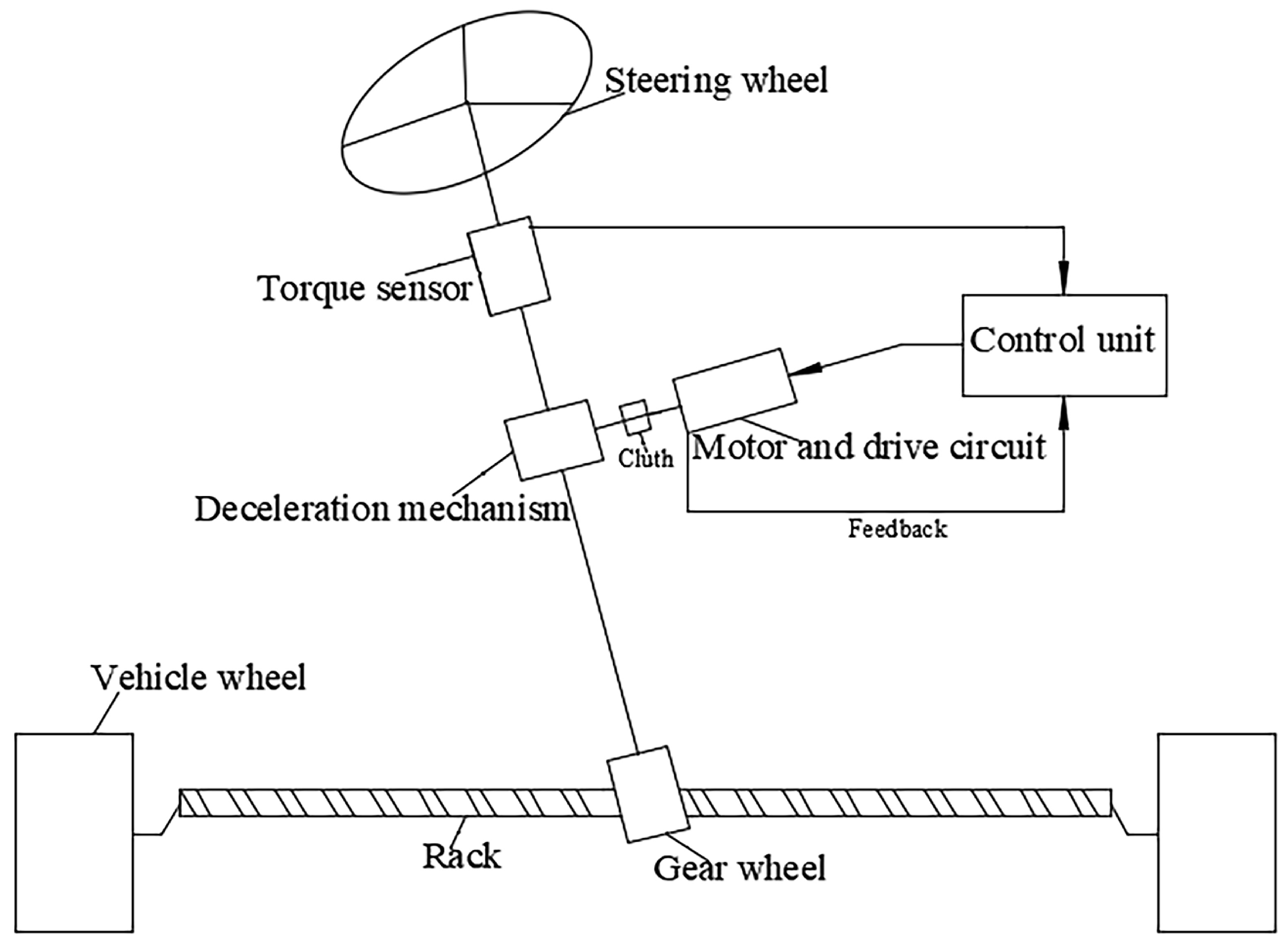
2. Dynamics Model of Forklift EPS System

According to the mechanical and electrical characteristics and parameters of the EPS system of the TFC35 forklift provided by Hefei Banyitong Science and Technology Development Co., Ltd., the EPS dynamic model and vehicle model are built to simulate and control the electric forklift 3-DOF model.

The dynamics model of EPS establishes the relationship between the steering mechanism, the electrodynamics of the motor and the tire/road contact force. A steering mechanism model equipped with a brush permanent magnet DC motor is shown in Figure 1.

According to Newton’s laws of motion, the equation of motion can be written as follows (Formulas (1)–(3) and

Table 1. The variables of Equations (1)–(3).

Symbol	Description	Values or Units
${\theta }_c$	Steering column angle	rad
${\theta }_m$	Motor angle	rad
$K_t$	DC motor torque constant	0.0506 (N∙m)/A
$K_m$	Back electromotive force constant	0.051 (V∙s/rad)
$M_r$	The mass of the steering rack	32 kg
$B_r$	The damping of the steering rack	3620 (N∙m)/rad
$K_r$	The stiffness of the steering rack	46,000 N/m
$J_c$	The rotational inertia of the steering column	0.089 kg
$B_c$	The damping of the steering column	0.361 (N∙m∙s)/rad
$K_c$	The stiffness of the steering column	115 (N∙m)/rad
$J_m$	The rotational inertia of the DC motor	0.00045 kg∙m2
$B_m$	The damping of the DC motor	0.0033 (N∙m∙s)/rad
$I_m$	The current of the DC motor	A
$R_m$	The resistance of the DC motor	0.345 Ω
$L_m$	The inductance of the DC motor	0.00023 H
$U_m$	DC motor voltage	V
$T_d$	Steering wheel torque	N∙m
$F_r$	Steering resistance moment	N∙m
$R_P$	The radius of steering gear wheel	0.4 m
$g_l$	The transmission ratio of deceleration mechanism	16.5

):

$$J_c{\ddot{\theta }}_c+B_c{\dot{\theta }}_c=T_d+K_c\frac{{\theta }_m}{g_l}-K_c{\theta }_c$$

(1)

$$\left(J_m+\frac{R_P^2}{g_l{}^2}{M}_r\right){\ddot{\theta }}_m+\left(B_m+\frac{R_p^2}{g_l{}^2}{B}_r\right){\dot{\theta }}_m=K_t{I}_m+K_c\frac{{\theta }_c}{g_l}-\left(\frac{K_c}{g_l{}^2}+\frac{K_r{R}_p^2}{g_l{}^2}{B}_r\right){\theta }_m-\frac{R_P}{g_l}{F}_r$$

(2)

$$U_m={\dot{I}}_m{L}_m+I_m{R}_m+K_m{\dot{\theta }}_m$$

(3)

Let ${\theta }_c,{\dot{\theta }}_c,{\theta }_m,{\dot{\theta }}_m,\mathrm{and}{I}_m$ represent the state variables in the motion process of the EPS system of the forklift, let $\epsilon \left(t\right)={\left[T_d{F}_r\right]}^T,\mathrm{and}u=\left[U_m\right],{\theta }_c,{\dot{\theta }}_c,T_c,{\dot{\theta }}_m,I_m$ represent the output of the EPS system of the forklift in the process of movement; the following is the form of state space of the EPS system of the forklift:

$$\{\begin{array}{l}\dot{x}\left(t\right)=Ax\left(t\right)+Bu\left(t\right)+M\epsilon \left(t\right)\\ y\left(t\right)=Cx\left(t\right)\end{array}$$

(4)

where

$$A=\left[\begin{array}{ccccc}0& 1& 0& 0& 0\\ -\frac{K_c}{J_c}& -\frac{B_c}{J_c}& \frac{K_c}{J_c{g}_l}& 0& 0\\ 0& 0& 0& 1& 0\\ \frac{g_l{K}_c}{g_l^2{J}_m+R_p^2{M}_r}& 0& -\frac{B_r{R}_p^2{K}_r+K_c}{g_l^2{J}_m+R_p^2{M}_r}& -\frac{R_p^2{B}_r+g_l^2{B}_m}{g_l^2{J}_m+R_p^2{M}_r}& \frac{g_l^2{K}_t}{g_l^2{J}_m+R_p^2{M}_r}\\ 0& 0& 0& -\frac{K_m}{L_m}& -\frac{R_m}{L_m}\end{array}\right]$$

$$B=\left[\begin{array}{c}0\\ 0\\ 0\\ 0\\ \frac{1}{L_m}\end{array}\right]$$

$$M=\left[\begin{array}{cc}0& 0\\ \frac{1}{J_c}& 0\\ 0& 0\\ 0& \frac{g_l{R}_P}{g_l^2{J}_m+R_p^2{M}_r}\\ 0& 0\end{array}\right]$$

$$C=\left[\begin{array}{ccccc}1& 0& 0& 0& 0\\ 0& 1& 0& 0& 0\\ K_c& 0& -\frac{K_c}{g_l}& 0& 0\\ 0& 0& 0& 1& 0\\ 0& 0& 0& 0& 1\end{array}\right]$$

3. Actuator Fault Model of EPS System

In this paper, the actuator fault is divided into power motor fault, deceleration mechanism, gear and rack actuator fault. Because the power motor drives the deceleration mechanism and the gear and rack movement, the power motor fault is defined as active actuator fault, and the deceleration mechanism and gear and rack faults are defined as passive actuator faults.

In this paper, actuator failure means that the actuator cannot complete the expected action. When the actuator fails, the EPS system cannot complete the ideal power steering. Common actuator faults are mainly divided into three categories: gain variation faults (multiplicative faults), constant deviation faults (additive faults) and stuck faults (constant output of the actuator). Stuck faults include two kinds of failure: complete failure and out of control. Complete failure refers to the motor voltage being constant zero, or the motor voltage is not zero, but it and the deceleration mechanism or the deceleration mechanism and gear rack is stuck, unable to move the failure state. Out of control refers to the motor suddenly running at a constant non-zero speed. At present, only the redundant hardware can achieve the purpose of fault tolerance, which will not be considered in this paper. In this paper, gain variation faults and constant deviation faults, namely, partial faults, are considered. Partial faults refer to the motor being in a controlled state, but the voltage loss or friction increase efficiency becomes low, or the deceleration mechanism and gear and rack wear lead to efficiency loss, that is, the actual steering power cannot reach the ideal steering power.

The main factors leading to motor fault and what kinds of fault types it will produce are:

• if the motor temperature is too high, it may lead to partial faults or stuck faults;
• if the air is damp, dusty and polluted, it may lead to partial faults or stuck faults;
• if there is no plug, the motor is broken, the motor is locked, it will lead to stuck faults;
• if the connection shorts between the wire harness end line and the ground, it will lead to stuck faults;
• if the converter is short circuited or open circuited, it will lead to stuck faults;

The main factors that lead to the failure of the deceleration mechanism, the gear and rack and what kinds of fault types it will produce are:

• if the clearance of the turbine worm is too large, it will lead to partial faults;
• if the tooth surface of the turbine worm is worn and the gear and rack are worn, it will lead to partial faults.

The following mathematical formula of actuator fault type corresponds to the list above. According to the fault estimation, we can judge what kind of fault has occurred. In practical engineering, because different factors can lead to the same type of fault, even if we know the fault type, we need to find out what factors caused it one by one.

The output of different types of fault actuators is uniformly described as follows:

$$u_q=\beta u\left(t\right)+u_0$$

(5)

where $\beta$ represents the gain variation coefficient of the actuator, $u_0$ represents the value of constant deviation fault or stuck fault of the actuator, and $u\left(t\right)$ represents the output of the normal actuator.

• when$\beta =1 \mathrm{and} u_0=0$, it is in a normal state and the actuator has no failure;
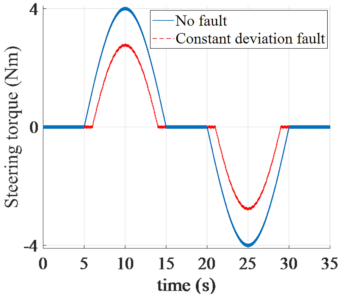
• when$\beta =1 \mathrm{and}{u}_0\ne 0$, it is a constant deviation fault and belongs to partial failure;
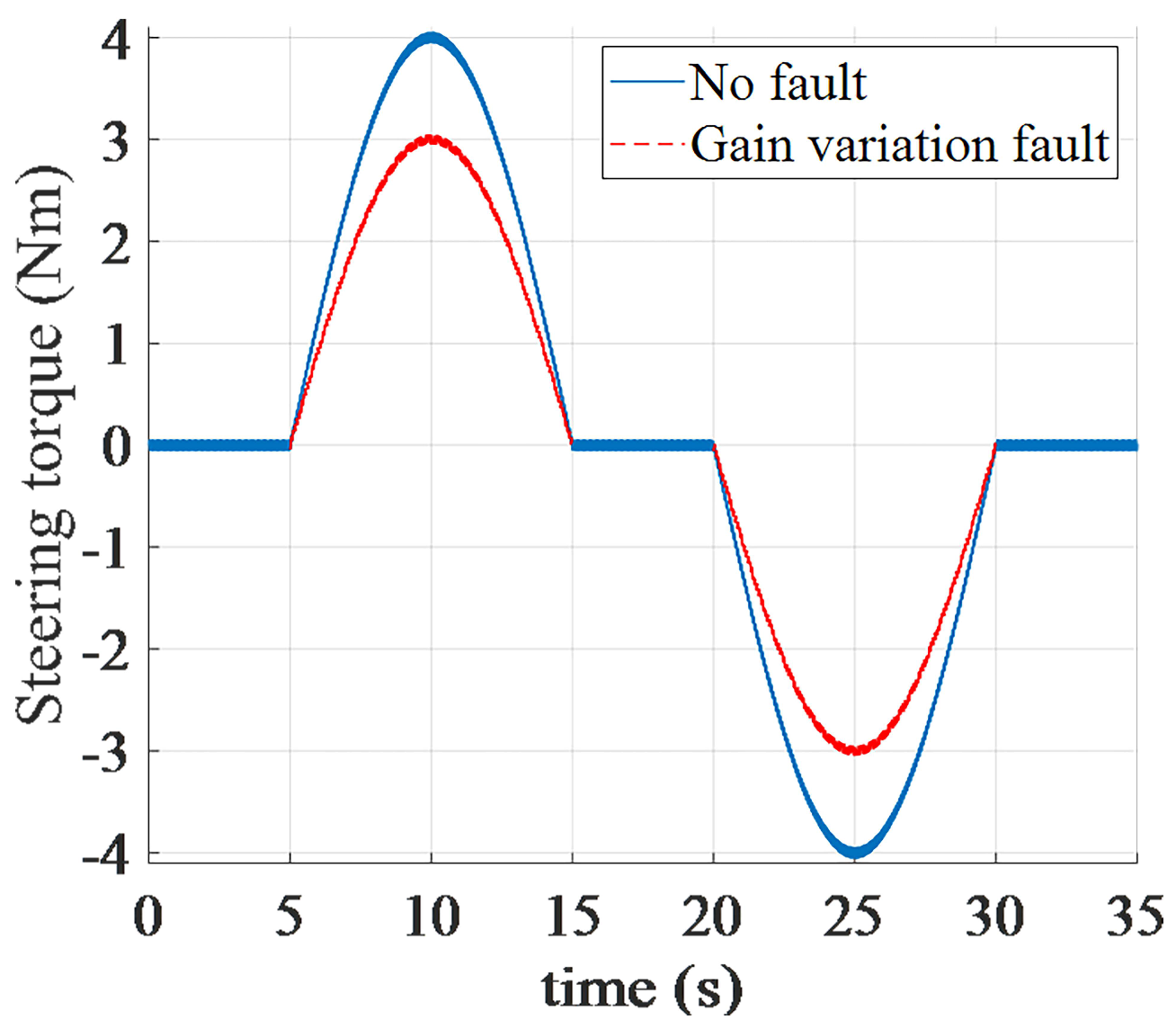
• when$0<\beta <1 \mathrm{and} u_0=0$, in this case, it is a gain variation fault and belongs to a partial failure;
• when $0<\beta <1 \mathrm{and}{u}_0\ne 0$, in this case, it is a mixed fault with constant deviation and gain variation and belonging to partial failure;
• when$\beta =0 \mathrm{and}{u}_0=0$, then the actuator has no output and is in a complete failure;
• when$\beta =0 \mathrm{and}{u}_0\ne 0$, the output of the actuator is a constant.

To isolate the fault items, the output of the fault actuator can be transformed as follows:

$$u_q=u\left(t\right)+\left[\left(\beta -1\right)u\left(t\right)+u_0\right]=u\left(t\right)+f_a\left(t\right)$$

(6)

then, we can obtain the actuator failure:

$$f_a\left(t\right)=\left(\beta -1\right)u\left(t\right)+u_0$$

(7)

Since the DC motor voltage $U_m$ is used as the control input $u\left(t\right)$ in this paper, the expression form of actuator fault $f_a\left(t\right)$ also needs to be converted into the voltage form. The fault type, time and law can be obtained through FDI unit, and the fault information of the power motor, deceleration mechanism and gear and rack can be collected and converted into the form of voltage. Moreover, if all states of the system are available, FTC design only needs to carry out FE. In practical engineering, the actuator of EPS system will become worse with the increase in service time, as shown in $u_q<u\left(t\right)$. In this paper, the most frequent actuator partial failure fault is considered, which is manifested as the actual steering power cannot reach the ideal steering power, the power motor loses voltage, leading to the steering power becoming smaller and cannot reach the ideal steering power; the actuator partial failure fault can be converted into the power motor voltage loss.

4. Integrated FE/FTC

4.1. System Description

Considering actuator faults and system interference, the fault model of EPS system is expressed as follows:

$$\{\begin{array}{l}\dot{x}\left(t\right)=Ax\left(t\right)+Bu\left(t\right)+F{f}_a\left(t\right)+D\epsilon \left(t\right)\\ y\left(t\right)=Cx\left(t\right)\end{array}$$

(8)

where $x\left(t\right)\in R^n$ is the system state vector; $u\left(t\right)\in R^m$ is input vector for the system; $y\left(t\right)\in R^p$ is the system measurable output; $\epsilon \left(t\right)\in R^l$ is the interference; $f_a\left(t\right)\in R^q$ is the actuator fault vector; $A\in R^{n\times n},B\in R^{n\times m},C\in R^{p\times n},D\in R^{n\times l},\mathrm{and}F\in R^{n\times q}$ are the known constant matrix. The following hypotheses on the system (8) are made.

Hypothesis 1 (H1).

($A,C$) is observable, ($A,B$) is controllable and $rank\left(B,F\right)=rank\left(B\right)=m$.

Hypothesis 2 (H2).

The $\epsilon \left(t\right)ϵ\left[0,\infty \right)$ and $f_a\left(t\right)ϵ\left[0,\infty \right)$, and $f_a\left(t\right)$ are continuously smooth with bounded first-time derivative.

Remark 1.

Hypotheses 1 and 2 are usually made for FE-based FTC systems with actuator faults. The condition $rank\left(B,F\right)=rank\left(B\right)=m$ ensures that the influence of the fault can be compensated by controlling the input.

The actuator fault is defined as an auxiliary state system, then System (8) is augmented into:

$$\{\begin{array}{l}\dot{\overline{x}}\left(t\right)=\overline{A}\overline{x}\left(t\right)+\overline{B}u\left(t\right)+\overline{D}\overline{\epsilon }\left(t\right)\\ y=\overline{C}\overline{x}\left(t\right)\end{array}$$

(9)

where $\overline{x}t=\left[\begin{array}{c}x\left(t\right)\\ f_a\left(t\right)\end{array}\right],\overline{A}=\left[\begin{array}{cc}A& F\\ 0& 0\end{array}\right],\overline{B}=\left[\begin{array}{c}B\\ 0\end{array}\right],\overline{C}=\left[\begin{array}{cc}C& 0\end{array}\right],\overline{D}=\left[\begin{array}{cc}D& 0\\ 0& I_q\end{array}\right],\overline{\epsilon }\left(t\right)=\left[\begin{array}{c}\epsilon \left(t\right)\\ {\dot{f}}_a\left(t\right)\end{array}\right]$.

Remark 2.

It can be verified below that the observability of Systems (8) and (9) is equivalent, since the matrix ($A,C$) is observable,

$$rank=\left[\begin{array}{c}s{I}_n-A\\ C\end{array}\right]=n,\forall s\in C,Re\left(s\right)\ge 0$$

which leads to

$$rank=\left[\begin{array}{c}s{I}_{n+q}-\overline{A}\\ \overline{C}\end{array}\right]=rank\left[\begin{array}{cc}s{I}_n-A& F\\ 0& s{I}_q\\ C& 0\end{array}\right]=n+q,\forall s\in C,Re\left(s\right)\ge 0$$

4.2. FE Design

The augmented state $\overline{x}\left(t\right)$ is estimated by a NUIO as follows:

$$\{\begin{array}{l}\dot{z}=Mz+Gu+Ly\\ \widehat{\overline{x}}=z+Hy\end{array}$$

(10)

where $z\in R^{n+q}$ is the observer system state and $\widehat{\overline{x}}\in R^{n+q}$ is the estimate of $\overline{x}$. The matrices $M\in R^{\left(n+q\right)\times \left(n+q\right)},G\in R^{\left(n+q\right)\times m},L\in R^{\left(n+q\right)\times p}, H\in R^{\left(n+q\right)\times q}$ are to be designed.

Defining the estimation error as $e=\overline{x}-\widehat{\overline{x}}$, the error dynamics as follows:

$$\dot{e}=\dot{\overline{x}}-\dot{\widehat{\overline{x}}}=\left(\Xi \overline{A}-L_1\overline{C}\right)e+\left(\Xi \overline{A}-L_1\overline{C}-M\right)z+\left(\Xi \overline{B}-G\right)u+\left[\left(\Xi \overline{A}-L_1\overline{C}\right)H-L_2\right]y+\Xi \overline{D}\overline{\epsilon }$$

(11)

where $\Xi =I_{n+q}-H\overline{C},L=L_1+L_2$, The matrices$M,G$,$\mathrm{and} L_2$ are defined as

$$M=\Xi \overline{A}-L_1\overline{C}, G=\Xi \overline{B}, L_2=\left(\Xi \overline{A}-L_1\overline{C}\right)H$$

(12)

With the definition given in Equation (12), the error dynamics (11) become

$$\dot{e}=\left(\Xi \overline{A}-L_1\overline{C}\right)e+\Xi \overline{D}\overline{\epsilon }$$

(13)

Theorem 1.

There exists a robust NUIO (10) if the error System (13) is robustly asymptotically stable.

Proof with Equation (12), the error System (13) is equivalent to the original error System (11). So, if Equation (13) is robustly and asymptotically stable, then Equation (11) is also robustly and asymptotically stable, indicating that $li{m}_{t\to \infty }e\left(t\right)=0$ in the presence of disturbance.

Note that the design matrices $M, G$ and $L$ can be derived after the matrices $L_1 \mathrm{and} H$ are obtained. Therefore, the main task of obtaining the NUIO (10) as described in the sequel is to design $L_1 \mathrm{and} H$ such that Equation (13) is robustly and asymptotically stable.

Remark 3.

Note from Equation (13) that the disturbance is completely decoupled from the state/FE if the following one condition holds: (Q) rank ($CD$) = rank ($D$) + $q$. The disturbance can be completely decoupled by designing $H$ such that $(I_{n+q}-H\overline{C})\overline{D}=0$ with $rank\left(\overline{C}\overline{D}\right)=rank\left(\overline{D}\right)$. Considering the case of partially decoupled disturbance, the method allows disturbance of the partial decoupling process in the observer design. An augmented state vector composed of current state, delay state and additive fault is constructed, and the augmented system is described inthe singular form. Then, an unknown input observer which can decouple some disturbances is obtained, and the uncoupled disturbances are reduced, but only one kind of integral measurement system is studied [14]. A robust NUIO (10) is proposed in this paper using $H_{\infty }$ optimization. This optimization method has no requirement of rank, so it is suitable for more practical engineering systems.

Remark 4.

It is worth noting that unlike traditional FDI, the traditional FDI includes fault detection and isolation processes based on residual generators, and the residual threshold is used to design the proposed NUIO to directly estimate the fault shape when faults occur. The observer can estimate the faults naturally and regard them as new states in an enhanced system.

In the proposed NUIO, the faults are assumed to be bounded and continuously smooth, and it is seen from Equation (13) that the FE performance is affected by the fault modelling error ${\dot{f}}_a$. The augmented perturbation $\overline{\epsilon }$ is not completely decoupled but attenuated by robust design. Thus, the robust FE performance depends on the robustness of the error System (11).

Remark 5.

Since the matrix $C$ in this paper is not the identity matrix, it can be assumed that

$$C=C_1+C_2=\left[\begin{array}{ccccc}1& 0& 0& 0& 0\\ 0& 1& 0& 0& 0\\ 0& 0& 1& 0& 0\\ 0& 0& 0& 1& 0\\ 0& 0& 0& 0& 1\end{array}\right]+\left[\begin{array}{ccccc}0& 0& 0& 0& 0\\ 0& 0& 0& 0& 0\\ K_c& 0& -1-\frac{K_c}{g_l}& 0& 0\\ 0& 0& 0& 0& 0\\ 0& 0& 0& 0& 0\end{array}\right].$$

It can be seen that the third row in $\widehat{\overline{x}}$ is $y_3=K_c \ast x_1-\frac{K_c}{g_l} \ast x_3$. Experimentation can be performed by comparing the value of the third row of $\widehat{\overline{x}}$ to the value of $K_c \ast x_1-\frac{k_c}{g_l} \ast x_3$; at the same time, the experimental results show that the fault estimation can estimate the system state well where $x={\left[x_1 x_2 x_3 x_4 x_5 \right]}^T$.

Remark 6.

Although the actuator fault is assumed to be continuously smooth with a bounded first-time derivative, it is not required to be differentiable everywhere. For any piecewise continuous fault $f_0\in R^{q_0}$ and a stable matrix $A_f\in R^{q_0\times q_0}$, there always exists an input vector $\omega \in R^{q_0}$ such that ${\dot{f}}_0=A_f{f}_0+\omega$. Therefore, following a similar design process, the proposed observer can also be used to estimate piecewise continuous faults.

4.3. Adaptive Sliding Mode FTC Design

A sliding surface for the System (8) is designed as follows:

$$s_1=N_1\widehat{x}$$

(14)

where $s_1\in R^m,\widehat{x}\in R^n$ is the estimate of system state $x$, and $N_1=B^{+}-Y_1\left(I_n-B{B}^{+}\right)$ with $B^{+}={\left(B^{T}B\right)}^{-1}{B}^T$ and an arbitrary matrix $Y_1\in R^{m\times n}$. Define the state estimation error as $e=x-\widehat{x}$. Differentiating $s_1$ with respect to time gives

$${\dot{s}}_1=N_{1}Ax+u+N_{1}F{f}_a+N_{1}D\epsilon -N_1{\dot{e}}_x$$

(15)

Design the control input as

$$u=u_l+u_n$$

(16)

where the linear feedback component is $u_l=-K\widehat{\overline{x}}$ with a design matrix. $K=\left[\begin{array}{cc}{K}_x& E_1\end{array}\right]$, $K_x\in R^{m\times n}$ is to be determined while $E_1=B^{+}F$. The nonlinear component is designed as follows:

$$u_n=\{\begin{array}{l}-{\rho }_{s_1}\left(t\right)\frac{s_1}{\Vert s_1\Vert } , s_1\ne 0\\ 0, s_1=0\end{array}$$

$\Vert ·\Vert$ represents the Euclidean norm of a vector and the induced norm of a matrix. With ${\rho }_{s_1}\left(t\right)={\widehat{\eta }}_{s_1}+{\phi }_{s_1}+{\delta }_{s1}$, ${\phi }_{s_1}>0,{\delta }_{s1}>0$ are design constants. The scalar ${\widehat{\eta }}_{s_1}$ is introduced to estimate ${\eta }_{s_1}$ which is defined as ${\eta }_{s_1}=\Vert N_{1}D\Vert {\epsilon }_0+\Vert E_1\Vert \left({\overline{f}}_a+\Vert {\widehat{f}}_a\Vert \right)+\Vert K_x\Vert e_{x_0}+N_1{\overline{e}}_{x_0}$, where $e_{x_0}$ and ${\overline{e}}_{x_0}$ are unknown scalars assumed to be upper bounds of $\Vert e_x\Vert$ and $\Vert {\overline{e}}_x\Vert$, respectively. The update law of ${\widehat{\eta }}_{s_1}$ is ${\dot{\widehat{\eta }}}_{S_1}={\sigma }_1\Vert s_1\Vert , {\widehat{\eta }}_{s_1}\left(0\right)>0$, with a learning rate ${\sigma }_1>0$ to be designed.

Define the estimation error of ${\eta }_{s_1}$ as ${\tilde{\eta }}_{s_1}={\eta }_{s_1}-{\widehat{\eta }}_{s_1}$ and consider a Lyapunov function

$$V_{s_1}=\frac{1}{2}\left(s_1^T{s}_1+\frac{1}{\sigma }{\tilde{\eta }}_{s_1}^2\right)$$

It follows from Equations (15) and (16) that

$${\dot{V}}_{s_1}=s_1^T{\dot{s}}_1-\frac{1}{{\sigma }_1}{\tilde{\eta }}_{s_1}{\dot{\widehat{\eta }}}_{s_1}\le \left({\omega }_{s_1}\Vert x\Vert +{\eta }_{s_1}-{\rho }_{s_1}\left(t\right)\right)\Vert s_1\Vert -{\tilde{\eta }}_{s_1}\Vert s_1\Vert \le ({\omega }_{s_1}\Vert x\Vert -{\phi }_{s_1}-{\delta }_{s1})\Vert s_1\Vert$$

where ${\omega }_{s_1}=\Vert N_{1}A-K_x\Vert +\Vert N_1{M}_0\Vert N_0$. By choosing ${\phi }_{s_1}>{\omega }_{s_1}{\varphi }_{s_1}$, with some scalar ${\varphi }_{s_1}>0$, it follows that the reaching and sliding conditions are satisfied, that is $s_1^T{\dot{s}}_1\le -{\delta }_{s1}\Vert s_1\Vert$ in the subset ${\Omega }_{s_1}=\left\{x:\Vert x\Vert \le {\varphi }_{s_1}\right\}$. Thus, the controller (16) ensures that if $x\left(0\right)\in {\Omega }_{s_1}$, then for all $t>\Vert s_1\left(0\right)\Vert /{\delta }_{s1},s_1={\dot{s}}_1=0$.

The stability analysis of the system corresponding to the sliding mode is considered. It is assumed that the system has been controlled to remain in the sliding mode (14). Substituting the equivalent control

$$u_{eq}=-\left(N_{1}Ax+N_{1}D\overline{\epsilon }\right)+u_l$$

(17)

into System (8) gives the closed-loop system

$$\dot{x}=\left(\Theta A-B{K}_x\right)x+B{K}_e+\Theta D\overline{\epsilon }$$

(18)

where $\Theta =I_n-B{N}_1$.

Therefore, by designing $K_x$ such that (18) is robustly stable, then the System (8) is maintained on the sliding mode with the equivalent control (17).

4.4. Integrated Synthesis of FE/FTC

The augmented closed-loop system composed of (13) and (18) is

$$\begin{gathered} \dot{x}=({\Theta }_{1}A-B{K}_x)x+B{K}_e+D_1\overline{\epsilon } \\ \dot{e}=\left(\Xi \overline{A}-L_1\overline{C}\right)e+\Xi \overline{D}\overline{\epsilon } \\ {z}_1=C_{x}x+C_e\mathrm{e} \end{gathered}$$

(19)

where $z_1ϵR^r$ is the measured output used to verify the closed-loop system performance with matrices $C_xϵR^{r\times n}, C_eϵR^{r\times \left(n+q\right)}, D_1=\left[\begin{array}{cc}\Theta D& 0\end{array}\right]$.

It can be seen from (19) that the system disturbance affects the state/FE, and the estimation error directly affects the control system. This shows that there is a bi-directional robustness interaction between the FE and FTC models, which breaks the so-called Separation Principle and produces an integrated FE/FTC design approach to achieve optimal and robustness overall performance of the FTC system. Now, the problem of integrated design can be expressed as follows: design the controller gain $K_x$ and the observer gains $H$ and $L_1$ to ensure the robust stability of the augmented closed-loop System (19).

This integrated design is essentially an observer-based robust control problem. To solve this problem, a one-step LMI formulation is proposed in Theorem 2. This one-step approach is modified from the method used in [23].

Theorem 2.

Given positive scalars ${\gamma }_1, {ϵ}_1, {ϵ}_2, {ϵ}_3, {\delta }_1 and {\delta }_2$, the closed-loop System (19) is stable with $H_{\infty }$ performance $\Vert G_{z_1\overline{d}}\Vert {}_{\infty }<{\gamma }_1$, if there exist three symmetric positive definite matrices $Z\in R^{n\times n},Q\in R^{n\times n},R\in R^{q\times q}$, and matrices $M_1\in R^{m\times n},M_2\in R^{n\times p},M_3\in R^{n\times p},M_4\in R^{q\times p},M_5\in R^{q\times p}$ such that

$$\left[\begin{array}{cc}{\Pi }_1& {\Pi }_2\\ \ast & {\mathsf{\Pi }}_3\end{array}\right]<0$$

(20)

with

$${\Pi }_1=\left[\begin{array}{cc}{\Xi }_{1,1}& {\Xi }_{1,2}\\ \ast & J_{2,2}\end{array}\right], {\Pi }_2=\left[\begin{array}{cccccccc}{\Xi }_{1,3}& {\Xi }_{1,4}& 0& {\Xi }_{1,6}& {\Xi }_{1,7}& 0& 0& {\Xi }_{1,10}\\ J_{2,3}& J_{2,4}& J_{2,5}& 0& 0& I& J_{2,9}& 0\end{array}\right]$$

$${\Pi }_3=-diag\left\{{\gamma }_1{}^{2}I,I,{ϵ}_{1}I,{\left({ϵ}_1+{ϵ}_2\right)}^{-1}I,{ϵ}_3{}^{-1}Z,{ϵ}_{3}Z,{\delta }_{1}I,{\left({\delta }_2{L}_f^2\right)}^{-1}I\right\}$$

$$J_{2,2}=\left[\begin{array}{cc}{\Xi }_{2,2}& {\Xi }_{2,3}\\ \ast & {\Xi }_{3,3}\end{array}\right], J_{2,3}=\left[\begin{array}{cc}QD-M_{2}CD& 0\\ -M_{4}CD& R\end{array}\right], J_{2,4}=\left[\begin{array}{c}{C}_{\mathrm{e}x}^{\top }\\ C_{\mathrm{e}fa}^{\top }\end{array}\right]$$

$$J_{2,5}=\left[\begin{array}{c}Q{M}_0-M_{2}C{M}_0\\ -M_{4}C{M}_0\end{array}\right], J_{2,9}=\left[\begin{array}{cc}Q-M_{2}C& 0\\ -M_{4}C& R\end{array}\right],$$

$$\begin{gathered} {\Xi }_{1,1}=He\left(\Theta AZ-B{M}_1\right)+{ϵ}_2{}^{-1}{M}_0{M}_0{}^{\top }+{\delta }_2{}^{-1}\Theta {\Theta }^{\top }, {\Xi }_{1,2}=\left[\begin{array}{cc}0& F\end{array}\right], \\ {\Xi }_{1,3}=\left[\begin{array}{cc}\Theta D& 0\end{array}\right], \end{gathered}$$

$${\Xi }_{1,4}=Z{C}_x^{\top }, {\Xi }_{1,6}=Z{N}_0^{\top }, {\Xi }_{1,7}=B{M}_1, {\Xi }_{1,10}=Z, {\Xi }_{2,2}=He\left(QA-M_{2}CA-M_{3}C\right)+{\delta }_1{L}_f^2{I}_n$$

$${\Xi }_{2,3}=QF-M_{2}CF-A^{\top }{C}^{\top }{M}_4^{\top }-C^{\top }{M}_5^{\top }, {\Xi }_{3,3}=He\left(-M_{4}CF\right).$$

where $He\left(W\right)=W+W^T,$ ‘$\ast$’ denotes the symmetric part of a matrix. Then the gains are given by

$$K_X=M_1{Z}^{-1},H_1=Q^{-1}{M}_2,H_2=R^{-1}{M}_4,L_{11}=Q^{-1}{M}_3,L_{12}=R^{-1}{M}_5$$

Proof Consider a Lyapunov function $V_e={\mathrm{e}}^{\top }{P}_1\mathrm{e}$ with a symmetric positive matrix $P_1$. The time derivative of $V_e$ along (13) is as follows:

$${\dot{V}}_e={\dot{e}}^{\top }{P}_{1}e+e^{\top }{P}_1\dot{e}=e^{\top }He\left[P_1\left(\Xi \overline{A}-L_1\overline{C}\right)\right]e+He\left(e^{\top }{P}_1\Xi \overline{D}\overline{\epsilon }\right)$$

(21)

Consider another Lyapunov function $V_x=x^{\top }{P}_{1}x.$ Then, the time derivative of $V_x$ along (18) is

$${\dot{V}}_x={\dot{x}}^{\top }{P}_{1}x+x^{\top }{P}_1\dot{x}=x^{\top }He\left[P\left(\Theta A-B{K}_x\right)\right]x+He\left(x^{\top }PBKe\right)+He\left(x^{\top }P{D}_1\overline{\epsilon }\right)$$

(22)

The $H_{\infty }$ performance $G_{z_1\overline{\epsilon }}<\gamma$ can be represented as

$$J={{\displaystyle \int }}_0^{\infty }\left(z_1^{\top }{z}_1-{\gamma }_1^2{\overline{\epsilon }}^{\top }\overline{\epsilon }\right)dt<0$$

(23)

Under zero initial conditions, it follows that

$$\begin{gathered} J={{\displaystyle \int }}_0^{\infty }\left(z_1^{\top }{z}_1-{\gamma }_1^2{\overline{\epsilon }}^{\top }\overline{\epsilon }+{\dot{V}}_x+{\dot{V}}_e\right)dt-{{\displaystyle \int }}_0^{\infty }\left({\dot{V}}_x+{\dot{V}}_e\right)dt \\ ={{\displaystyle \int }}_0^{\infty }\left(z_1^{\top }{z}_1-{\gamma }_1^2{\overline{\epsilon }}^{\top }\overline{\epsilon }+{\dot{V}}_x+{\dot{V}}_e\right)dt-\left(V_x(\infty )+V_e(\infty )\right)+\left(V_x\left(0\right)+V_e\left(0\right)\right) \\ \le {{\displaystyle \int }}_0^{\infty }\left(z_1^{\top }{z}_1-{\gamma }_1^2{\overline{\epsilon }}^{\top }\overline{\epsilon }+{\dot{V}}_x+{\dot{V}}_e\right)dt \end{gathered}$$

A sufficient condition for the satisfaction of (23) is

$$J_1=z_1^{\top }{z}_1-{\gamma }_1^2{\overline{\epsilon }}^{\top }\overline{\epsilon }+{\dot{V}}_x+{\dot{V}}_e<0$$

(24)

Substituting (21) and (22) into (24) yields

$$J_1={\left[\begin{array}{c}x\\ e\\ \overline{\epsilon }\end{array}\right]}^{\top }\left[\begin{array}{ccc}{J}_{11}& PBK& P{D}_1\\ \ast & J_{22}& P_1\Xi \overline{D}\\ \ast & \ast & -{\gamma }_1^{2}I\end{array}\right]\left[\begin{array}{c}x\\ e\\ \overline{\epsilon }\end{array}\right]<0$$

(25)

where $J_{11}=He\left(P\left(\Theta A-B{K}_x\right)\right)+{\delta }_2^{-1}P\Theta {\Theta }^{\top }P+{\delta }_2{L}_f^2{I}_{\mathrm{n}}+\left({ϵ}_1+{ϵ}_2\right)N_0^{\top }{N}_0+$${ϵ}_2{}^{-1}P{M}_0{M}_0^{\top }P+C_x^{\top }{C}_x, J_{22}=He\left(P_1\left(\Xi \overline{A}-L_1\overline{C}\right)\right)+{\delta }_1^{-1}{P}_1\Xi {\Xi }^{\top }{P}_1+{\delta }_1{L}_f^2{A}_0^{\top }{A}_0{I}_{n+q}+{ϵ}_1{}^{-1}{P}_1\Xi {\overline{M}}_0{\overline{M}}_0^{\top }{\Xi }^{\top }{P}_1$$++C_e^{\top }{C}_e$.

Define $Z=P^{-1}$. Pre-multiplying and post-multiplying both sides of (25) with diag($Z, I, I$) gives

$$\left[\begin{array}{ccc}{J}_{11}& BK& D_1\\ \ast & J_{22}& P_1\Xi \overline{D}\\ \ast & \ast & -{\gamma }_1^{2}I\end{array}\right]<0$$

(26)

where $J_{11}=He\left(\left(\Theta A-B{K}_x\right)Z\right)+{\delta }_2^{-1}\Theta {\Theta }^{\top }+{\delta }_2{L}_f^{2}ZZ+\left({ϵ}_1+{ϵ}_2\right)Z{N}_0^{\top }{N}_{0}Z+{ϵ}_2{}^{-1}{M}_0{M}_0^{\top }+Z{C}_x^{\top }{C}_{x}Z,$$J_{22}=He\left(P_1\left(\Xi \overline{A}-L_1\overline{C}\right)\right)+{\delta }_1^{-1}{P}_1\Xi {\Xi }^{\top }{P}_1+{\delta }_1{L}_f^2{A}_0^{\top }{A}_0{I}_{n+q}+{ϵ}_1{}^{-1}{P}_1\Xi {\overline{M}}_0{\overline{M}}_0^{\top }{\Xi }^{\top }{P}_1++C_e^{\top }{C}_e$.

It follows from the Young’s relation that for some positive scalar ${ϵ}_3$,

$$\mathrm{He}\left\{\left[\begin{array}{c}B{K}_x\\ 0\\ 0\end{array}\right]{\left[\begin{array}{c}0\\ I\\ 0\end{array}\right]}^{\top }\right\}\le {ϵ}_3\left[\begin{array}{c}B{K}_{x}Z\\ 0\\ 0\end{array}\right]Z^{-1}{\left[\begin{array}{c}B{K}_{x}Z\\ 0\\ 0\end{array}\right]}^{\top }+{ϵ}_3{}^{-1}\left[\begin{array}{c}0\\ I\\ 0\end{array}\right]Z^{-1}{\left[\begin{array}{c}0\\ I\\ 0\end{array}\right]}^{\top }$$

Further define

$$P_1=\left[\begin{array}{cc}{Q}_{n\times n}& 0\\ 0& R_{q\times q}\end{array}\right],L_1=\left[\begin{array}{c}{L}_{11}\\ L_{12}\end{array}\right],H=\left[\begin{array}{c}{H}_1\\ H_2\end{array}\right]$$

$$M_1=K_{x}Z,M_2=Q{H}_1,M_3=Q{L}_{11},M_4=R{H}_2,M_5=R{L}_{12}.$$

Using the Schur complement repeatedly, (26) can be finally reformulated into (20).

Remark 7.

The nonlinear term $PB{K}_x$ in (25) is linearized by introducing an equality constraint, and the integral FE/FTC problem is solved by using a one-step LMI formula. This equality constraint imposes some restriction on the systems (e.g., the matrix B has to be full column) and some requirements on the Lyapunov matrix $P$ [5]. Here, the requirement of equation constraint is removed by using the Young’s relation, which provides more flexibility for optimal design. However, it should also be pointed out that this LMI formulation has a more prescribed design scalar ${ϵ}_3$ for solving the LMI (20).

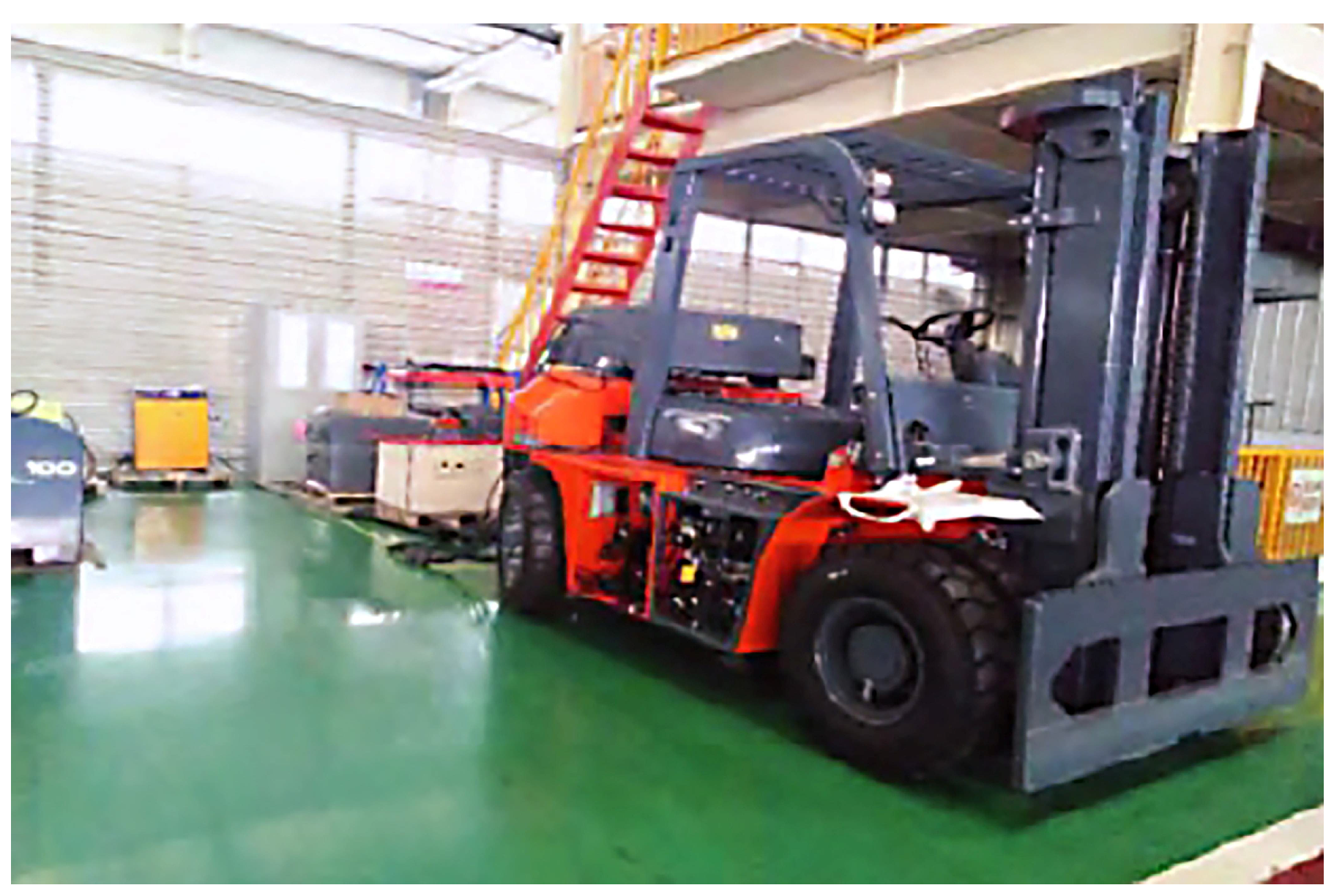
5. Experimental Verification

We used a TFC35 forklift provided by Hefei Banyitong Science and Technology Development Co., Ltd. (Hefei, China) as the research object, and the data of the power motor, deceleration mechanism, rack, gear and steering torque of EPS system are collected. The wheel speed sensor, the torque sensor and the current sensor were installed during the experiment. The experiment was carried out in a warehouse with an indoor relative humidity of 20%. The experimental platform is shown in Figure 2. The speed of the forklift is ${\mathrm{v}}_{\mathrm{u}}=15\mathrm{km}/\mathrm{h}$. The LMI toolbox in MATLAB is used to solve the observer gain matrix $L, G, H, M$ and the controller gain $K_x$. The experiment was conducted manually. In the process of the experiment, the calculated information is loaded into the controller chip dsPIC33EP, and the data acquisition card collects the actuator information. The controller receives the sensor signal and regulates the steering torque by power motor voltage which is calculated by the NUIO and adaptive sliding mode algorithm.

In order to verify the effectiveness of the proposed integrated FE and FTC method, FE/FTC is integrated for the most frequent actuator partial failure faults. For complete failure and out-of-control cases, the FTC can only be achieved through redundant hardware at present.

Figure 3, Figure 4 and Figure 5 show the collected steering torque information, including the no-fault condition and the fault condition. The fault value is added manually, such as reducing the motor voltage, increasing the gap between the deceleration mechanism, the rack and the gear and increasing the wear. If actuator failure occurs, the steering torque will change at this time. On the contrary, according to the collected power torque information, we can also judge what fault will occur at this time. Figure 3, Figure 4 and Figure 5 pave the way for the subsequent actuator failure. According to Equations (5) and (6), the output expressions of different types of fault actuators are:

$$u_q=\beta u\left(t\right)+u_0=u\left(t\right)+f_a\left(t\right)$$

when $\beta =1,u_0\ne 0$, it is constant deviation fault and belongs to partial failure fault; if the actuator has a constant deviation fault, the steering torque is shown in Figure 3.

When $0<\beta <1,u_0=0$, it is a gain variation fault and belongs to a partial failure fault; if the actuator has a gain variation fault, the steering torque is shown in Figure 4.

When $0<\beta <1,u_0\ne 0$, it is a constant deviation and gain variation mixed fault, belonging to partial failure fault; if the actuator has hybrid faults with constant deviation and gain variation, the steering torque is shown in Figure 5.

For the above three faults, suppose that the ideal power assist torque we need is: $T_d=4sin\left(0.4\pi t\right)$. Ideally, the power torque is proportional to the power motor voltage, that is $u\left(t\right)=4K\ast sin\left(0.4\pi t\right) \left(K\ne 0\right)$, just for the verification experiment, so $K$ is going to be 1. The system has the following actuator failure and distribution matrix. In order to satisfy hypothesis 1, and according to references [4,5,6], in order to ensure that the influence of fault can be well compensated by control input, it is assumed that matrix $F$ is equal to matrix $B$. The values of the actuator faults need be set manually according to Figure 3, Figure 4 and Figure 5. Additionally, according to the actuator failure, Equation (7):

$$f_a\left(t\right)=\left(\beta -1\right)u\left(t\right)+u_0$$

Failure case 1. When $\beta =1,u_0\ne 0$, we take $u_0=-1$, this corresponds to the situation in Figure 3, then the constant deviation fault is as follows:

$$f_a\left(t\right)=\{ \begin{array}{c}0 0\le t<5 \\ -1 5\le t<45\\ 0 45\le t<50\end{array}$$

Failure case 2. When $0<\beta <1,u_0=0$, we take $\beta =0.75, \beta =0.9$. This corresponds to the situation in Figure 4, then the gain variation fault is as follows:

$$f_a\left(t\right)=\{\begin{array}{c} 0 0\le t<5\\ (0.75-1)u\left(t\right)=-0.25u\left(t\right)=-\sin \left(0.4\pi t\right) 5\le t<25\\ (0.9-1)u\left(t\right)=-0.1u\left(t\right)=-0.4\sin \left(0.4\pi t\right) 25\le t<50\end{array}$$

Failure case 3. When $0<\beta <1,u_0\ne 0$, we take $\beta =0.75$, $u_0=-1$; this corresponds to the situation in Figure 5, then the hybrid faults with constant deviation and gain variation is as follows:

$$f_a\left(t\right)=\left(\beta -1\right)u\left(t\right)+u_0=\{\begin{array}{c} 0 0\le t<5\\ -sin\left(0.4\pi t\right)-1 5\le t<50\end{array}$$

It can be seen from Figure 6, Figure 7 and Figure 8 that in the process of the experiment, the fault estimation value of the actuator collected by the data acquisition card can track the fault setting curve accurately. We manually make the actuator produce some faults and collect the steering torque information, as shown in Figure 3, Figure 4 and Figure 5. The defined fault is generated again, and in the process of fault estimation, we use the data acquisition card to collect fault estimation information. The nonlinear unknown input observer proposed in this paper has good fault estimation results for actuator constant deviation faults, gain variation faults, and constant deviation and gain variation mixed faults, and the effect is better than that of the decentralized design. The fault estimation error of the integrated design actuator is smaller than that of the decentralized design. In this paper, the fault estimation can estimate the system states, and then take a look at some system states.

As can be seen from Figure 9, the integrated FE/FTC design has a faster response and better control effect to actuator faults than the decentralized design, ensuring the robust stability of the closed-loop system.

Assume that the speed of the forklift is $v_u=15\mathrm{km}/\mathrm{h}$, the input sinusoidal torque of the driver is $T_d=3sin\left(0.4\pi t\right)$ and the input torque period of the driver is 10 s, as shown in Figure 10. The integrated FTC test and decentralized FTC test were carried out when the actuator gain change fault occurred at 12.5 s in the EPS system. The integrated FTC test and decentralized FTC test were carried out when the EPS system was fault-free and the EPS system was fault-tolerant at the same time. As shown in the figure, when a fault occurs, the power torque of the EPS system fault is quickly restored to the power torque value of the EPS system without faults. At the same time, the integrated design is faster and better than the decentralized design, so as to reflect the improvement of the reliability of the integrated FTC on the EPS system. In the same way, real vehicle tests were carried out for the actuator constant deviation fault and the mixed fault of constant deviation and gain variation, and the results were consistent with the fault of gain variation.

6. Conclusions

For forklift EPS systems affected by bounded disturbance and actuator faults, a rank-free NUIO algorithm is proposed to estimate the system state and fault simultaneously, and an adaptive sliding mode FTC controller is constructed by using the obtained estimates. The integrated design is compared with the decentralized design. The integrated FE/FTC design problem is expressed as an observer-based robust control problem, which is solved by using $H_{\infty }$ optimization in the one-step LMI formula. By considering the two-way robust interaction between the FE model and the FTC model, the integrated design achieves good FE/FTC performance. The integrated design scheme and integrated design can accurately estimate the fault of the actuator and ensure the robust stability of the closed-loop system. The FTC system has realized well the power-assisted performance of the electric forklift actuator in the case of faults. Finally, the effectiveness of the proposed method is verified by the experimental results of a real vehicle.

References

1. Joubaneh Eshagh, F.; Oumar, B. A comprehensive study of vibration suppression and optimization of an electric power steering system. SAE Int. J. Veh. Dyn. Stab. NVH 2021, 5, 81–97. [Google Scholar] [CrossRef]
2. Zhang, Z.L.; Xiao, B.X. Sensor Fault diagnosis and fault tolerant control for forklift based on sliding mode theory. IEEE Access 2020, 8, 84858–84866. [Google Scholar] [CrossRef]
3. Tao, J.; Xiao, B.X. Fault tolerant control of actuator and sensor in EPS system of electric forklift. J. Electron. Meas. Instrum. 2019, 33, 85–93. [Google Scholar]
4. Lan, J.L.; Patton, R.J. Integrated fault estimation and fault-tolerant control for Lipschitz nonlinear systems. Int. J. Robust Nonlinear Control 2017, 27, 761–780. [Google Scholar] [CrossRef]
5. Lan, J.L.; Patton, R.J. A new strategy for integration of fault estimation within fault-tolerant control. Automatica 2016, 69, 48–59. [Google Scholar] [CrossRef]
6. Zhao, X.Y.; Zong, Q.; Tian, B.; Liu, W.J. Integrated fault estimation and fault-tolerant tracking control for Lipschitz nonlinear Multiagent Systems. IEEE Trans. Cybern. 2020, 50, 678–688. [Google Scholar] [CrossRef]
7. Ghimire, R.; Sankavaram, C.; Ghahari, A.; Pattipati, K. Integrated model-based and data-driven fault detection and diagnosis approach for automotive electric power steering system. IEEE Autotestcon 2011, 70–77. [Google Scholar] [CrossRef]
8. Gao, Z.F.; Zhou, Z.P.; Jiang, G.P.; Qian, M.S.; Lin, J.X. Active fault tolerant control scheme for satellite attitude systems: Multiple Actuator Faults Case. Int. J. Control. Autom. Syst. 2018, 16, 1794–1804. [Google Scholar] [CrossRef]
9. Yuan, Y.; Zhang, T.H.; Lin, Z.L.; Zhao, Z.W.; Zhang, X.L. Actuator fault tolerant control of variable cycle engine using sliding mode control scheme. Actuators 2021, 10, 24. [Google Scholar] [CrossRef]
10. Liu, C.; Qian, K.; Li, Y.H.; Ding, Q. Design of integrated robust active fault tolerant controller based on LMI. Control. Decis. 2018, 33, 53–59. [Google Scholar]
11. Navarbaf, A.; Javad Khosrowjerdi, M. Fault-tolerant controller design with fault estimation capability for a class of nonlinear systems using generalized Takagi-Sugeno fuzzy model. Trans. Inst. Meas. Control. 2019, 41, 4218–4229. [Google Scholar] [CrossRef]
12. Qin, Y.F.; Shi, X.J.; Zhai, Y.Y.; Han, L.; Long, Y.F. Based on the ASTSMO and UIO the method of fault estimation. J. Beijing Univ. Aeronaut. Astronaut. 2020, 46, 2253–2263. [Google Scholar]
13. Mousavi, A.; Markazi, M.; Amir, H.D. A predictive approach to adaptive fuzzy sliding-mode control of under-actuated nonlinear systems with input saturation. Int. J. Syst. Sci. 2021, 52, 1599–1617. [Google Scholar] [CrossRef]
14. Liu, Y.; Wang, Z.D.; Zhou, D.H. State estimation and fault reconstruction with integral measurements under partially decoupled disturbances. IET Control. Theory Appl. 2017, 12, 1520–1526. [Google Scholar] [CrossRef]
15. Huang, C.; Naghdy, F.; Du, H. Observer-based fault-tolerant controller for uncertain steer-by-wire systems using the delta operator. IEEE Trans. Mechatron. 2018, 23, 2587–2598. [Google Scholar] [CrossRef]
16. Garramiola, F.; del Olmo, J.; Poza, J.; Madina, P.; Almandoz, G. Integral sensor fault detection and isolation for railway traction drive. Sensors 2018, 18, 1543. [Google Scholar] [CrossRef] [PubMed] [Green Version]
17. Djeziri, M.A.; Merzouki, R.; Bouamama, B.O.; Ouladsine, M. Fault diagnosis and fault-tolerant control of an electric vehicle overactuated. IEEE Trans. Veh. Technol. 2013, 62, 986–994. [Google Scholar] [CrossRef]
18. Wang, Z.H.; Shen, Y.; Zhang, X.L. Actuator fault estimation for a class of nonlinear descriptor systems. Int. J. Syst. Sci. 2014, 45, 487–496. [Google Scholar] [CrossRef]
19. Yan, Y.; Wu, L.B.; Zhao, N.N.; Zhang, R.Y. Adaptive asymptotic tracking fault-tolerant control of uncertain nonlinear systems with Actuator Failures and Event-triggered Inputs. Int. J. Control. Autom. Syst. 2021, 19, 1241–1251. [Google Scholar] [CrossRef]
20. Tavasolipour, E.; Poshtan, J.; Shamaghdari, S. A new approach for robust fault estimation in nonlinear systems with state-coupled disturbances using dissipativity theory. ISA Trans. 2021, 114, 31–43. [Google Scholar] [CrossRef]
21. Yang, J.Q.; Zhu, F.L.; Wang, X.; Bu, X.H. Robust sliding-mode observer-based sensor fault estimation, actuator fault detection and isolation for uncertain nonlinear systems. Int. J. Control. Autom. Syst. 2015, 13, 1037–1046. [Google Scholar] [CrossRef]
22. Ljaz, S.; Chen, F.Y.; Tariq Hamayun, M. A New Actuator Fault-Tolerant Control for Lipschitz Nonlinear System Using Adaptive Sliding Mode Control Strategy; John Wiley & Sons, Ltd.: Hoboken, NJ, USA, 2021; Volume 31, pp. 2305–2333. [Google Scholar]
23. Odgaard, P.F.; Stoustrup, J. Fault Tolerant Control of Wind Turbines using Unknown Input Observers. IFAC Proc. Vol. 2012, 45, 313–318. [Google Scholar] [CrossRef] [Green Version]
24. Witczak, M.; Buciakowski, M.; Aubrun, C. Predictive actuator fault-tolerant control under ellipsoidal bounding. Int. J. Adapt. Control Signal Process. 2016, 30, 375–392. [Google Scholar] [CrossRef]
25. Kheloufi, H.; Zemouche, A.; Bedouhene, F.; Souley-Ali, H. A robust H observer-based stabilization method for systems with uncertain parameters and Lipschitz nonlinearities. Int. J. Robust Nonlinear Control. 2016, 26, 1962–1979. [Google Scholar] [CrossRef]
Figure 1. EPS mechanism model.
Applsci 11 07236 g001
Figure 2. Experimental platform.
Applsci 11 07236 g002
Figure 3. Constant deviation fault.
Applsci 11 07236 g003
Figure 4. Gain variation fault.
Applsci 11 07236 g004
Figure 5. Hybrid faults with constant deviation and gain variation.
Applsci 11 07236 g005
Figure 6. (a) True and estimated fault values in fault case 1; (b) fault case 1 fault estimation error.
Applsci 11 07236 g006
Figure 7. (a) True and estimated fault values in fault case 2; (b) fault case 2 fault estimation error.
Applsci 11 07236 g007
Figure 8. (a) True and estimated fault values in fault case 3; (b) fault case 3 fault estimation error.
Applsci 11 07236 g008
Figure 9. (a) Fault-tolerant control of motor angular position; (b) fault-tolerant control of motor angular velocity.
Applsci 11 07236 g009
Figure 10. Fault-tolerant control of the gain variation fault.
Applsci 11 07236 g010