Prediction of Dynamic Responses of Flow-Induced Vibration Using Deep Learning

Abstract

Flow-induced vibration (FIV) is a phenomenon in which the flow passing through a structure exerts periodic forces on the structure. Most studies on FIVs focus on suppressing this phenomenon. However, the Marine Renewable Energy Laboratory (MRELab) at the University of Michigan, USA, has developed a technology called the vortex-induced vibration for aquatic clean energy (VIVACE) converters that reinforces FIV and converts the energy in tidal currents to electrical energy. This study introduces the experimental data of the VIVACE converter and the associated method using deep neural networks (DNNs) to predict the dynamic responses of the converter. The DNN was trained and verified with experimental data from the MRELab, and the findings show that the amplitudes and frequencies of a single cylinder in the FIV predicted by the DNN under various test conditions were in good agreement with the experimental data. Finally, based on both the predicted and experimental data, the optimal power envelope of the VIVACE converter was generated as a function of the flow speed. The predictions using DNNs are expected to be more accurate as they can be trained with more experimental data in the future and will help to substantially reduce the number of experiments on FIVs.

1. Introduction

Interest in marine renewable energy has gradually been increasing worldwide, and various marine technologies have been developed for commercialization of the energy generated thereof. With more than 70% of the Earth’s surface covered by water, significant amounts of potential energy are stored in storm surges, sea waves, and resources in the form of heat and salts in the ocean. However, most marine renewable energy technologies have not yet been commercialized because of their low efficiencies and high cost of power generation compared to conventional fossil fuels. Recently, marine power generation technologies have been developed specifically for commercialization [1]. The vortex induced vibration for aquatic clean energy (VIVACE) converter, a marine renewable energy technology, converts the hydrokinetic energy in water to electrical energy [2]. The VIVACE converter was invented and patented by the Marine Renewable Energy Laboratory (MRELab) at the University of Michigan and was developed based on the simple idea of maintaining and enhancing vortex-induced vibrations (VIVs) while maximizing flow-induced vibration (FIV), rather than suppressing them. Several lab-scale converters have been built and tested in the low-turbulence free surface water (LTFSW) channel at the MRELab since 2005 [2]. The research team has been investigating methods to improve the power output of the converter by enhancing the FIVs of multiple cylinders over a wide range of flow speeds. For this study, the MRELab provided the experimental data of a single-cylinder converter to train our deep neural network (DNN) to predict the dynamic responses and power outputs of the converter.

FIVs are caused in various structures, such as bridges, buildings, and offshore structures resulting from fluid flows. One of the most common types of FIVs is the VIV, which was first observed by Leonardo da Vinci in 1504 [3].

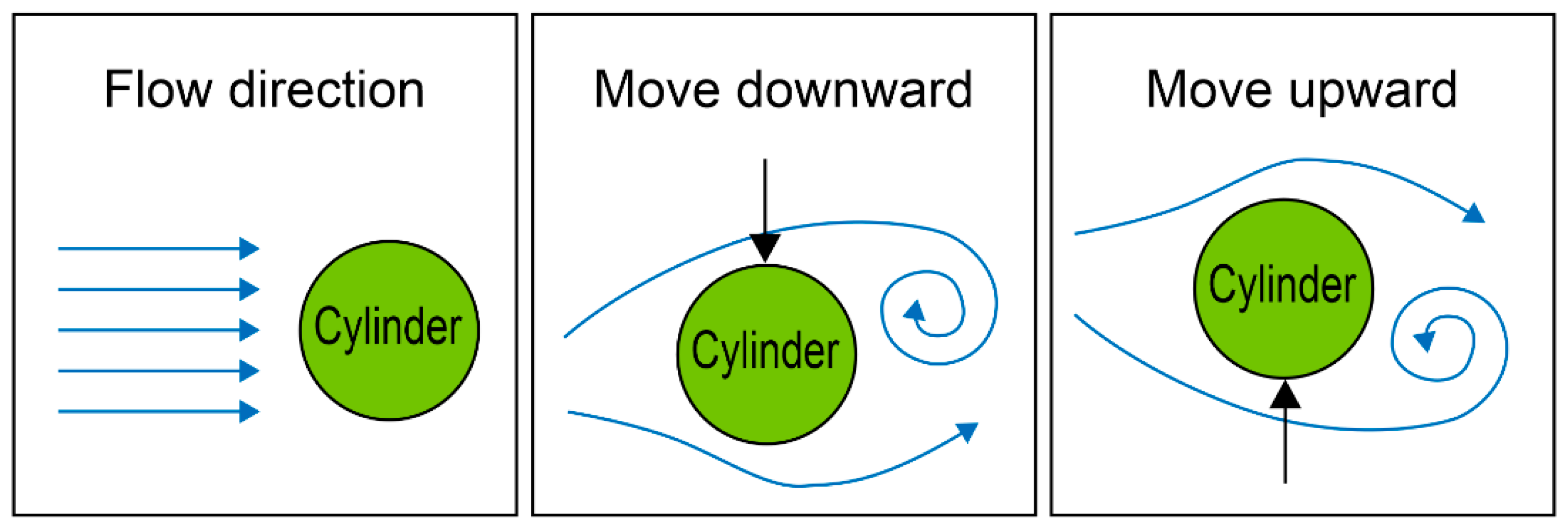
VIV is generally caused by alternate vortex shedding on both sides of the cylinder like Figure 1, which causes periodic lift forces to act on the cylinder. Galloping is another type of FIV that has a lower frequency and a larger amplitude compared to VIV and is caused by the asymmetric motions of the shear layers. Galloping is a more powerful phenomenon than VIV and can occur for a cylinder with noncircular cross sections above a certain critical flow speed. The amplitude of the galloping continues to increase with the flow velocity until the structure is destroyed. In general, as the flow velocity increases, VIVs occur first, followed by galloping. Because of the destructive nature of FIVs in structures, most researchers have focused on its suppression. In 2006, however, the MRELab research team developed the VIVACE converter, where the kinetic energy of the fluid could be converted to electrical energy by enhancing and controlling the FIVs [4,5,6].

This study is concerned with predicting the amplitude and frequency of a single cylinder installed in the VIVACE converter by learning the FIV experiment data through a deep learning model. The study was conducted using experimental data provided by MRELab. When a neural network learns the test data and a deep learning model is constructed to predict the dynamic responses of FIVs for different conditions without learning, the results can be confirmed within a relatively short time. In addition, learning the experimental data under various conditions can be an alternative to statistical methods, such as regression analysis [7].

Therefore, in recent research, studies have been actively conducted on the system to predict data measured via experiments or with sensors by learning the deep learning model. Deep learning can be used not only for interpretation of incomplete and noisy input data but also for pattern recognition, classification, generalization, and abstraction while learning of large amounts of data [8]. In addition, the prediction model through data-based learning is highly applicable as it learns and builds the model relationships with key input and output variables compared to performance predictions using the traditional dynamic simulation tools [9].

To train the different conditions and variables used in the experiment, data preprocessing steps, such as data regularization, were performed, and a deep learning model was constructed. To predict the amplitude and frequency of the cylinder as the output value, optimization was performed by adjusting the hyperparameters of the deep learning model. Using the deep learning model prediction responses of FIVs, we can reduce the number of experiments substantially and produce the optimal power envelope of the VIVACE converter more efficiently. The concepts and techniques of VIVACE using FIVs used in this study are described in Section 2. Section 3 describes data preprocessing and training in the development of deep learning models to predict the dynamic response of FIVs. Section 4 decides on a new optical power envelope by verifying the dynamic response results of FIVs using the deep learning model and predicting untested data.

2. Power Generation Technology of VIVACE Converter Using FIVs

Contrary to previous efforts to suppress FIVs, which can destroy structures subject to fluid flows, the VIVACE converter utilizes and even enhances FIVs to harness the power from rivers and currents. The first prototype of the converter was developed at the end of 2003 and tested at MRELab in 2004. The left side of Figure 2 shows the schematic of the simplest unit of the VIVACE converter, comprising a single circular cylinder suspended by springs and a power take-off system. On the right side of Figure 2, four of the units installed on the LTFSW channel at the MRELab are shown [10].

The experiments were conducted in the flow range of 30,000 < Re < 120,000 for the Reynolds number (Re) to harness the optimal power envelopes at various flow velocities [12]. The Reynolds number is defined by:

$$Re=\frac{U D}{\nu }$$

where U, D, and $\nu$ are the free stream velocity, the diameter of a circular cylinder, and the kinematic viscosity of fresh water, respectively.

All tests with the single cylinder with passive turbulence control (PTC) presented herein were performed in the LTFSW channel of the MRELab. The measured turbulence intensity of the test section normalized by the free stream velocity was reported lower than 0.1% [1,4,6,10] and it is suitable for the experiments [13]. A virtual spring-damping (Vck) system, a servo-motor controller that replaces physical damping and springs were designed and built to investigate the effects of damping and spring stiffness on power generation [11]. A schematic of the design model is shown in Figure 3.

The first VIVACE converter was intended to utilize only VIV, as implied by the name. Because of the self-limiting characteristics of the VIV phenomenon, the harness power of the single-cylinder VIVACE converter is limited by its lock-in range and the self-limiting VIV characteristics. However, previous works on FIVs in circular cylinders have shown that fluid dynamic changes caused by attachments to the cylinders can cause galloping in circular cylinders [14]. In contrast to VIV, galloping is a vibration type with a short period compared to its high amplitude in a single degree of freedom and generally occurs in noncircular cross sections. Galloping is caused by motion-aiding forces, resulting in very high amplitude motions with the total system damping falling below zero and induction of negative aero/hydrodynamic damping. To overcome the shortcomings of VIV and initiate galloping, the MRELab team extensively investigated the effects of passive turbulence control (PTC), which is applied in the form of roughness strips attached to the cylinders [10,12,15]. This study shows that the selectively applied roughness on the cylinder surface can cause significant changes in the properties of the boundary or shear layers; accordingly, the cylinder responses may change. 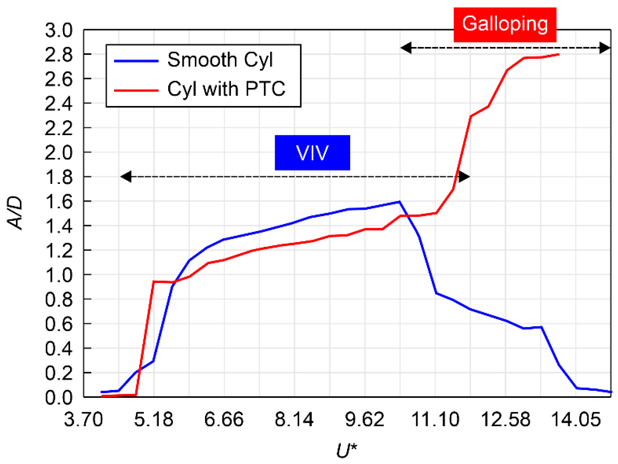For some PTC positions, as shown in Figure 4, the PTC extends the upper VIV branch point to the reduced velocity U* ≈ 11 and increases fully from U* ≈ 12. The reduced velocity is defined by:

$$U^{*}=\frac{U}{f_{nw}D}$$

The natural frequency of the system including added mass is defined by:

$$f_{nw}=\sqrt{\frac{K}{m_{osc}+m_{add}}}$$

where K, m_osc, and m_add are the spring stiffness, oscillating mass, and added mass, respectively.

The transition range in which both VIV and galloping mechanisms coexist is 11 < U* < 12. Therefore, the synchronization region of FIVs, which covers both the alternately occurring VIV and galloping, increases rapidly. Thus, the VIVACE converter was able to harness higher quantities of power at over a wide range of speeds from 0.38 m/s to 1.45 m/s and maximum speed of the LTFSW channel. An optimal harnessed power curve is created by superimposing the results of the harnessed power calculated from different combinations of the damping and spring stiffness values, as shown in Figure 5.

The optimal harnessed power of a cylinder with PTC is larger than that of a smooth cylinder in the synchronization region of VIV. Further, when the flow velocity exceeds 1.2 m/s, the harnessed power curve increases sharply, reaching 49.35 W at a flow velocity of 1.45 m/s for K = 2000 N/m and ζ_harness = 0.16; however, the smooth cylinder is asynchronous and can no longer supply power. The power calculated at 1.45 m/s is more than three times the maximum harnessed power of the smooth cylinder.

3. Deep Learning Model for Dynamic Response Prediction of FIVs

3.1. FIV Tested Data for Learning

Experiments were performed with the learning data using the second-generation Vck system developed by MRELab. Figure 6 shows the single-cylinder converter mounted in the LTFSW channel.

The Reynolds number in the range of 30,000 < Re < 120,000 and the flow velocity in the range of 0.395 m/s < U < 1.315 m/s were the tested data conditions used in this study. When the mass ratio (m* = m_osc/m_d) was 1.343, the spring constant (K) was 400, 600, 755, 1000, and 1200 N/m, and the harness damping ratio (ζ_harness) for each spring constant was 0.04, 0.08, 0.12, 0.16, 0.2, and 0.24.

Table 1. PTC parameters (P60).

Parameter	Value
Placement angle (αPTC, degree)	20
Angular coverage of strip (θ, degree)	16
Sandpaper plus tape thickness (P, mm)	0.587
Average grit height (k, mm)	0.26
Total thickness of strip (T − P + k, mm)	0.847

and Figure 7 show the results for the dynamic responses of a single rigid circular cylinder mounted with PTC [11,12,14]. In addition, the specifications of the single cylinder oscillator model, along with the tested conditions, are summarized in

Table 2. Particulars of single-cylinder oscillator model.

Particular	Value
K (N/m)	400	600	755	1000	1200
Temperature (°C)	20.5
μ (N∙s/m2)	1.004 × 10−3
ν (m2/s)	9.940 × 10−7
ρ (kg/m3)	999.72965
D (m)	0.0889
L (m)	0.89535
mdisplacement (kg)	5.425
moscillation (kg)	7.285775
madded (kg)	5.425
ζstructure	0.02
fn,water	0.893	1.093	1.227	1.412	1.546

.

Through testing under the above conditions, the parameters to train the tested data of the single-cylinder amplitude and natural frequency of the system for the deep learning model were first extracted. A total of six parameters were extracted, as follows: spring constant K, harness damping ratio of the system ζ_harness, number of rotations of the induction generator to circulate the water in the LTFSW channel f_motor, natural frequency of the cylinder in water, f_n,water, reduced velocity U*, and finally the Reynolds number Re. Correlation analysis was then performed to identify the effects of the extracted parameters on the dependent variables, amplitude (A/D), and frequency (f_cyl) of the cylinder. The correlation coefficient was calculated using the Pearson method in this study, which is a parametric correlation coefficient, as shown in

Table 3. Correlation analysis for selecting the independent variables (N = 714).

	K	ζharness	fmotor	fn,water	U*	Re	A/D	fcyl
K	1.000
ζharness	0.000	1.000
fmotor	0.030	0.000	1.000
fn,water	0.997	0.000	0.030	1.000
U*	−0.500	0.000	0.825	−0.508	1.000
Re	0.030	0.000	1.000	0.030	0.825	1.000
A/D	−0.244	−0.334	0.707	−0.246	0.755	0.707	1.000
fcyl	0.261	−0.177	0.277	0.260	0.065	0.277	0.473	1.000

.

Equation (1) shows the expression used to calculate the correlation coefficient of the Pearson method.

$$\begin{gathered} \mathrm{Pearson}\mathrm{Coefficient}\left(\mathrm{r}\right)=\frac{n{\displaystyle \sum }{X}_i{Y}_i-{\displaystyle \sum }{X}_i{\displaystyle \sum }{Y}_i}{\sqrt{n{\displaystyle \sum }{X}_i^2-{\left({\displaystyle \sum }{X}_i\right)}^2}\sqrt{n{\displaystyle \sum }{Y}_i^2-{\left({\displaystyle \sum }{Y}_i\right)}^2}} \\ \mathrm{where}\mathrm{X}=\mathrm{Independent}\mathrm{variable} \\ \mathrm{Y}=\mathrm{Dependent}\mathrm{variables} \\ \mathrm{n}=\mathrm{Number}\mathrm{of}\mathrm{specimens} \end{gathered}$$

(1)

The four input values of the deep learning model selected through correlation analysis were: K, ζ_harness, U*, and Re. The variables U* and Re were selected, which have large positive linear relationships with the amplitude of the cylinder. The variable K was added as it had a relatively large correlation, and there were no other variables that correlated with the frequency compared to the amplitude of the cylinder. Finally, by adding ζ_harness with a negative correlation coefficient to the amplitude and frequency of the cylinder, the four selected input parameters are obtained. For the output parameters, the amplitude ratio A/D of the cylinder in FIVs and the cylinder frequency, f_cyl, at the nodes of the output layer, respectively, were predicted.

We constructed a dataset of 667 cases by VIVACE converter results and a untested dataset of 647 cases. Most of the tested data of the VIVACE converter was used as Training data, and some as test data to verify the general performance of the trained model. After verifying the general performance of the trained network, we input the untested data to predict the amplitude and frequency of the cylinder. The contents of the data classification are summarized in

Table 4. Data classification for learning in deep learning models.

	Spring Constants (K)	ζharness for Training (No. of Training Data)	ζharness for Test (No. of Test Data)	Number of Total Data
Tested data by VIVACE converter	400	0.04, 0.08, 0.12, 0.16, 0.2, 0.24 (150)	-	150
	600	0.04, 0.08, 0.12, 0.2, 0.24 (120)	0.16 (24)	144
	755	0.04, 0.08, 0.12, 0.16, 0.2, 0.24 (138)	-	138
	1000	0.04, 0.08, 0.12, 0.2, 0.24 (115)	0.16 (23)	138
	1200	0.04, 0.08, 0.12, 0.16, 0.2, 0.24 (144)	-	144
Untested data	500	-	0.04, 0.08, 0.12, 0.16, 0.2, 0.24 (150)	150
	700	-	0.04, 0.08, 0.12, 0.16, 0.2, 0.24 (150)	150
	900	-	0.04, 0.08, 0.12, 0.16, 0.2, 0.24 (150)	150
	1100	-	0.04, 0.08, 0.12, 0.16, 0.2, 0.24 (150)	150
Total data		667	647	1314

.

3.2. Deep Learning Model Structure

The structure of the neural network is composed of an input layer, a hidden layer, and an output layer. Here, the input layer receives the external inputs, and the hidden layer is located between the input and output layers and invisible to the outside. The output layer provides the results processed by the last hidden layer [8,9,16].

In this study, the neural network shown in Figure 8 is constructed. A fully connected neural network structure consisting of one input layer, one output layer, and five hidden layers is used. The number of hidden layers and the nodes in the hidden layers were trained for the specifications shown in

Table 5. Learning condition.

Learning Condition	Range
Hidden layers	3,5,7,9
Nodes	Minimum of 48 to Maximum of 468
Batch sizes	256, 512, 1024
Learning rates	0.1, 0.01, 0.001
Epochs	10,000–50,000

, and the number of hidden layers and nodes with the lowest average error rate of the test data were selected.

For the input values of the deep learning model, four values were extracted through correlation analysis and entered. The output values predict the amplitude A/D and cylinder frequency f_cyl for the FIVs of the cylinder at the node of the output layer. The number of nodes for each hidden layer is set to 80 × 64 × 48 × 32 × 16. Finally, before learning the classified data, the input values were normalized to uniformly match the input values between 0 and 1 for all results [17], as expressed by Equation (2).

$$\begin{gathered} \overline{d}=\frac{d-\min v}{\max v-\min v} \\ where, \overline{d}=Normalized data \\ d=Data before normalize \\ \min v=Minimum value of the feature \\ \max v=Maximum value of the feature \end{gathered}$$

(2)

3.3. Deep Learning Model Training

In this study, cross-validation was used to learn the overall characteristics of the experimental data and increase the reliability of the generalization performances of the deep learning models. There are various cross-validation methods available; however, the repeated random subsampling validation method, using which the ratio between the training and validation sets is adjusted and not affected by the number of training data, is employed as shown in Figure 9.

The goal of the deep learning model optimization is to determine the values of the hyperparameters such that the learning of the neural network models and value of the loss function according to their results are minimized. Therefore, fine tuning was performed by controlling the number of nodes per hidden layer. The optimal number of nodes was selected by repeating the increase and decrease in the number of nodes. In addition, the hyperparameters, such as learning rate, iteration, and batch size, that affect the neural network were adjusted.

Then, the functions for learning the deep learning model were selected. The activation function converts the sum of the input signals into output signals, such as the step function used in perceptrons. At the nodes of the hidden layers, the sum of the linear product of the data and its weight are calculated, and the threshold is applied to obtain the activation level [18]. In this study, the rectified linear unit (ReLU) activation function was used [19,20]. Compared to the sigmoid function, which has been majorly used in the past, the ReLU can be implemented with a simple formula, and the function also resolves the vanishing gradient problem, which was considered as a chronic problem in the deep learning model [21]. The function is expressed as a graph in Figure 10 and as an equation in Equation (3).

$$f=\{\begin{array}{c}x<0, f\left(x\right)=0\\ x\ge 0, f\left(x\right)=x\end{array}$$

(3)

The optimization function accelerates the learning of the deep learning models and uses the Adam optimizer, which is efficient in terms of computational resources. The cost function uses the root mean square error (RMSE), and the He initialization is used for the weight initialization method. The He initialization method is to initialize the ReLU function and considers the characteristics of the input and output values rather than random initialization [22]. In this study, the He initialization method was used, as shown in Equation (4). The initialization for the ReLU activation function considers the characteristics of the input and output values, rather than random initialization. Depending on the characteristics of the data, when there were n nodes in the previous layer, a normal distribution with a square root of 2/n is used. This method was able to significantly increase the learning speed of the neural network, and it was confirmed that the loss function was reduced early in the learning process.

$$\begin{gathered} \mathrm{He}\mathrm{Normal}\mathrm{Initialization}\mathrm{W}~\mathrm{N}\left(0,\mathrm{Var}\left(\mathrm{W}\right)\right) \\ \mathrm{N}=\mathrm{Normal}\mathrm{distribution} \\ \mathrm{W}=\mathrm{Weight}\mathrm{beween}\mathrm{nodes} \\ \mathrm{Var}\left(\mathrm{W}\right)=\sqrt{\frac{ 2 }{ n_{in}+n_{out} }} \\ {n}_{in}{}^{ }=\mathrm{Number}\mathrm{of}\mathrm{nodes}\mathrm{in}\mathrm{the}\mathrm{previous}\mathrm{layer} \\ {n}_{out}{}^{ }=\mathrm{Number}\mathrm{of}\mathrm{nodes}\mathrm{in}\mathrm{the}\mathrm{next}\mathrm{layer} \end{gathered}$$

(4)

Learning was performed based on a batch size of 300. The learning rate determines the value of the weight that the neural network updates after learning. The deep learning model checks the RMSE every 1000 learnings and adjusts the learning rate and number of learning steps until the cost function is minimized. In the selection of the number of hidden layers, the greater the depth of the neural network hidden layer, the lower is the cost function. However, when the depth increased above a certain level, the cost function could not converge and showed divergence. In this study, the best-learned cost function with five hidden layers is shown in Figure 11, and the average error rate for each data structure of the neural network that completed learning is presented in

Table 6. Average error rate by data in a learned neural network.

	Error (%)	Train Average Error	Validation Average Error	Test Average Error *
Output
A/D		6.35	13.05	15.96
fcyl		3.12	8.47	11.29

* Only include Tested data by VIVACE converter.

.

* Only include Tested data by VIVACE converter.

4. Deep Learning Model Prediction

4.1. Prediction Results of Data Tested through VIVACE Converter

In this study, test data were applied to a deep learning model constructed using neural network learning to predict the dynamic responses of FIVs via deep learning. First, we investigated the results when ζ_harness = 0.16 at K = 600 and 1000 N/m extracted from the experimental data. It was confirmed that the predicted results of the test data applied to the learned neural network followed the trends of the VIV and galloping phenomena throughout the experiment. Figure 12 and Figure 13 below show the predicted results of cylinder amplitude and frequency of the test data extracted from the experimental data. The error rate was predicted to be within 5% compared with the actual experimental data. However, relatively large errors occurred in the initial section, where the VIV phenomenon started occurring, and the transition section from the VIV to the galloping section.

Next, the power curve obtained by the VIVACE converter was calculated using the predicted results of the amplitude and frequency of the cylinder. The equation used in the calculation is the actual equation used for the experiment with the VIVACE converter and is represented by Equation (5). Figure 14 shows the power curve of the VIVACE converter, which is calculated using the amplitude and frequency of the cylinder.

$$\begin{gathered} {\mathrm{Power}}_{harness}\left(W\right)=4{\pi }^2{\zeta }_{harness}\sqrt{K\ast m_{osc}}{\left(D\ast \frac{A}{D}\ast f_{cyl}\right)}^2 \\ {\zeta }_{harness}=\text{Harness damping ratio} \\ K=\text{Spring constant} \\ {m}_{osc}=\text{mass of oscilation} \\ D=\text{Cylinder diameter} \\ A=\text{Amplitude of cylinder} \\ {f}_{cyl}=\text{Frequency of cylinder} \end{gathered}$$

(5)

4.2. Prediction Results of Untested Data

In this study, we confirmed the validity of the power curves through experiments with the VIVACE converter and the above predicted results. Therefore, the amplitude and frequency of the cylinder were predicted for each input data ζ_harness in the learned neural network model in the range of K = 500, 700, 900, and 1100 N/m, which are in the untested range. Figure 15 shows the power curves, using which the optimal power envelope with the maximum power for each Re according to the flow velocity is shown in Figure 16. The optimal power envelope is a curve expressed to obtain the highest power generation and high efficiency by the Re, by considering the effects of the mass ratio, spring stiffness, and harness damping ratio. The combination curve is created by combining the experimental and predicted curves. By comparing the predicted optimal power curve using the deep learning model and optimal power curve prepared via the previous experiments, new K and ζ_harness values with optimal power were obtained when m* was 1.343.

Table 7. Parameters for optimal harness and converted power curve for combination power.

Re	K (N/m)	ζharness	Power (W)
35,292	400	0.12	0.7
38,869	400	0.12	1.0
42,447	600	0.16	1.5
46,024	600	0.2	3.0
49,602	700	0.24	4.3
53,179	700	0.24	5.3
56,756	900	0.24	7.0
60,334	900	0.24	8.4
63,911	1000	0.24	9.3
67,489	1200	0.24	9.2
71,066	1200	0.2	8.4
74,644	1200	0.12	4.9
78,221	1200	0.08	4.2
80,010	1200	0.08	3.5
81,799	1200	0.12	5.6
85,376	1200	0.12	6.8
88,954	1200	0.16	7.9
92,531	1200	0.16	8.5
96,109	1200	0.16	9.0
99,686	1200	0.2	9.9
103,264	700	0.24	10.7
106,841	700	0.24	11.6
110,418	700	0.24	12.5
113,996	1200	0.2	14.2
117,573	1200	0.2	16.8

lists the optimal power curve values that combine the experimental results of the VIVACE converter with those predicted through deep learning.

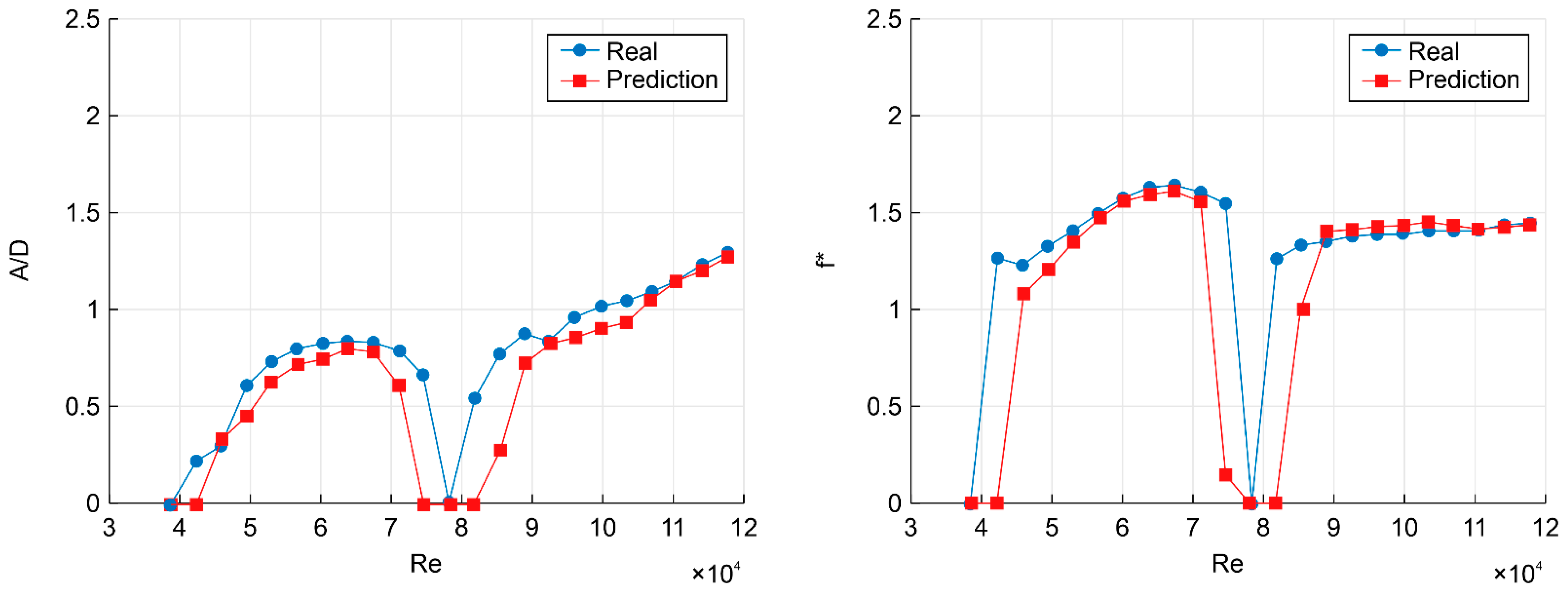
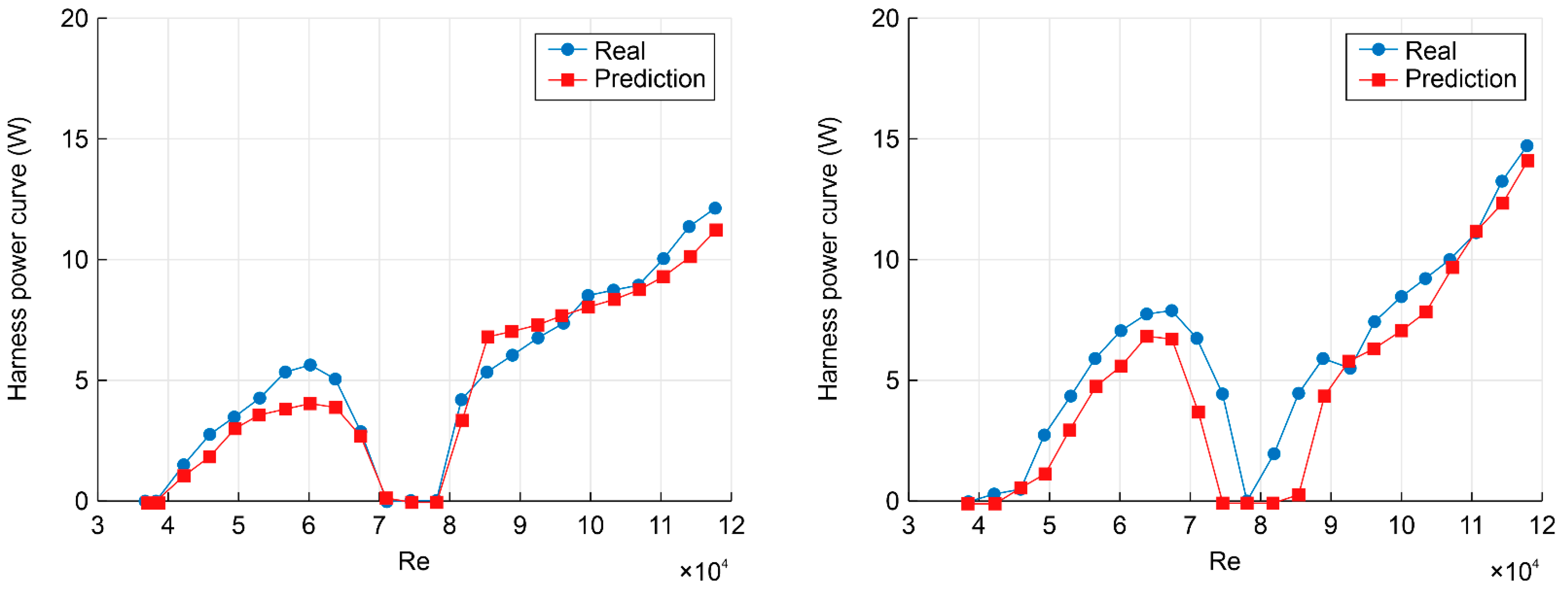
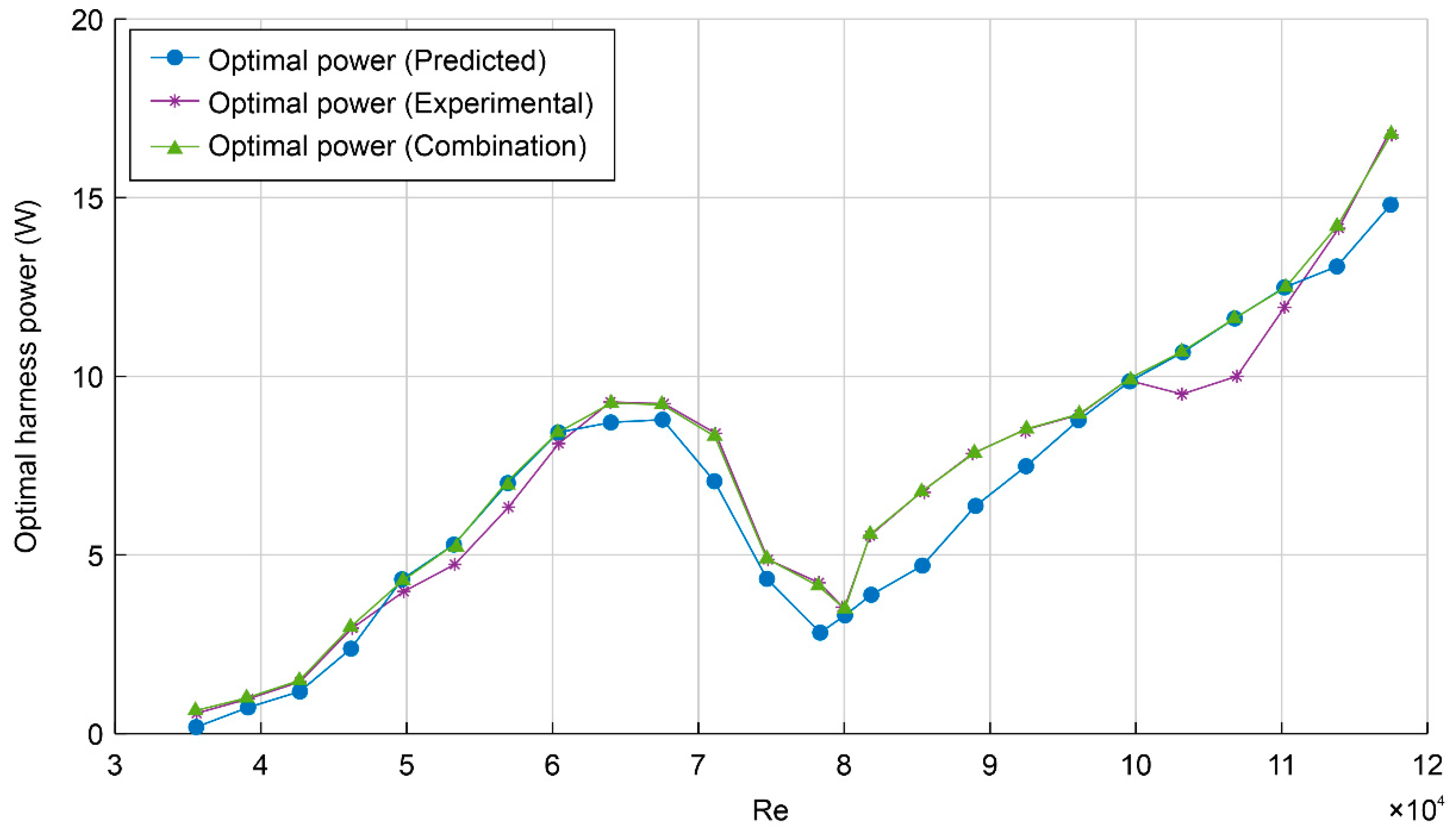
5. Conclusions

This study involved the development of a deep learning model that can predict the cylinder amplitudes and frequencies by training the FIV experimental data from the MRELab team with a neural network. Using four input values for deep learning model training, we performed data preprocessing, and the cylinder amplitudes and frequencies were predicted as output values. The experimental data obtained through the VIVACE converter was used as training data, with some used as test data to verify the generalization performance of the learned neural network. After validating the generalization performance of the network, the untested data were input to predict the cylinder amplitudes and frequencies of the VIVACE converter. The optimal power curves were calculated from the cylinder dynamic responses predicted by the deep learning model, and the results were compared with the experimental results. In conclusion, a new optimal harnessed power curve was created by combining the experimental results of the VIVACE converter and the predicted results through deep learning. The findings of the experimental study are thus summarized as follows:

(1)

The deep learning model was trained to predict the dynamic response of the cylinder amplitude and frequency. When compared with the actual experimental results, an average error rate of approximately 10% was observed for the mean values of the cylinder amplitude and frequency.

(2)

The optimal power curve was calculated using the amplitude and frequency of the cylinder predicted by deep learning. It was further verified by comparing with the actual experimental results, and the new optimal power envelope was created by the predicted dynamic response of the cylinder.

(3)

A new optimal harness power curve was created to obtain the maximum power according to the flow velocity when m* = 1.343, compared with the optimal power envelope calculated through the experiment.

(4)

A part of the experimental conditions was classified into test data and predictions were obtained using the deep learning model. The results confirmed the possibility of identifying the dynamic responses of the cylinder under the conditions experimented before the VIVACE converter experiment.

Based on the above results, the deep learning model adequately predicted the experimental results of the dynamic response of the cylinder in the VIVACE converter, but the error rate was rather large in the region where the initial VIV phenomenon occurred or in the transition region. These regions require various experimental data and research conditions because of the complexity of the phenomenon itself, which is difficult to accurately measure even in actual experiments. However, due to the complexity of the phenomenon itself, experimental data and research under various conditions are required to replace the experiment. While this study predicts the dynamic response for a single cylinder, it can be used to predict the dynamic response for each cylinder in an entire system with multiple cylinders. In the future, it is expected that this work will be helpful for the initial stage of experiments by learning the experimental data of the VIVACE converter under various conditions and calculating the optimum power in the early stages of the experiment in advance.