Determination and Quantification of Heavy Metals in Sediments through Laser-Induced Breakdown Spectroscopy and Partial Least Squares Regression

Abstract

Conventional analysis techniques and sample preprocessing methods for identifying trace metals in soil and sediment samples are costly and time-consuming. This study investigated the determination and quantification of heavy metals in sediments by using a Laser-Induced Breakdown Spectroscopy (LIBS) system and multivariate chemometric analysis. Principle Component Analysis (PCA) was conducted on the LIBS spectra at the emission lines of 11 selected elements (Al, Ca, Cd, Cr, Fe, K, Mg, Na, Ni, Pb, and Si). The results showed apparent clustering of four types of sediment samples, suggesting the possibility of application of the LIBS technique for distinguishing different types of sediments. Mainly, the Cd, Cr, and Pb concentrations in the sediments were analyzed. A data-smoothing method—namely, the Savitzky–Golay (SG) derivative—was used to enhance the performance of the Partial Least Squares Regression (PLSR) model. The performance of the PLSR model was evaluated in terms of the coefficient of determination (R²), Root Mean Square Error of Calibration (RMSEC), and Root Mean Square Error of Cross Validation (RMSECV). The results obtained using the PLSR with the SG derivative were improved in terms of the R² and RMSECV, except for Cr. In particular, the results for Cd obtained with the SG derivative showed a decrease of 25% in the RMSECV value. This demonstrated that the PLSR model with the SG derivative is suitable for the quantitative analysis of metal components in sediment samples and can play a significant role in controlling and managing the water quality of rivers.

1. Introduction

The construction of artificial impoundments has been on the rise over the last few decades. The construction of dams or weirs results in hydrologic alteration, which impacts trophic levels, sedimentation rates, and the quantity and quality of freshwater sediments [1,2,3,4]. The amount of sediments retained by impoundment structures has reached 4–5 Gt/yr, which corresponds to approximately 25–30% of the global land–ocean transfer of sediments by rivers [5]. An extensive river restoration project conducted in Korea during the period of 2010–2011 included the construction of weirs and the enlargement of river channels, which led to the dredging of a large amount of benthic sediment from riverbeds and riverside floodplains.

Sediments are important components in the study of heavy metal contamination in rivers because many contaminants and particle-reactive elements are eventually deposited in the bottom sediment [6,7]. Trace metals may reach water systems from lithogenic or anthropogenic sources, such as industrial waste, fossil fuel combustion, sewage wastewater, energy production, and construction. Because trace metals are mainly adsorbed and accumulated at the bottom of the sediments, the sediments act as both a sink and source of trace metals, which may be released again into water bodies through various remobilization processes, resulting in potential environmental and human health issues [8]. Hence, sediments can be used as indicators of local pollution.

Several analytical techniques, such as Atomic Absorption Spectrometry (AAS), X-ray fluorescence spectroscopy, and Inductively Coupled Plasma–Optical Emission Spectroscopy (ICP-OES), have been applied to the identification of trace metals in soil and sediment samples. Conventional analysis techniques and complicated sample preprocessing methods, such as fusion dissolution and microwave digestion, are costly and time-consuming. To overcome these limitations, we employed Laser-Induced Breakdown Spectroscopy (LIBS) as a fast and minimally destructive measurement technique for analyzing trace metals in sediments.

LIBS has been used in various fields, particularly for soil analyses. The authors of [9] applied LIBS to investigate the feasibility of detecting heavy metals in sand matrices. Dry synthetic sand samples were used in the test stage for a field application. The authors of [10] quantitatively identified the total content of heavy metals in reference soil samples by comparing their results with those obtained using Inductively Coupled Plasma (ICP) spectroscopy. The authors of [11] studied a set of heavy metals, particularly chromium, in soil and sewage sludge based on a constructed calibration curve. Furthermore, multivariate statistical analysis techniques coupled with LIBS were applied to reduce spectrum noise. The authors of [12] employed principal component analysis (PCA) for the discrimination of varieties of soil. The authors of [13] tested a calibration method and scatter diagram of principal components (PCs) to extract the correlation and discriminate between soils contaminated with heavy metals (or oils) and clean soils.

The objective of this study was to understand and evaluate heavy metal pollution in sediments by collecting surface sediments from the vicinity of weirs constructed across four rivers, considering that many potential pollutants in the sediments significantly influence the river environment. Multivariate chemometrics based on LIBS data were utilized for the determination and quantification of heavy metals in the sediments. PCA was applied to distinguish the characteristics of the sediment samples. The concentrations of heavy metals, particularly Cd, Cr, and Pb were evaluated by using the Savitzky–Golay (SG) derivative and partial least squares regression (PLSR) methods. For the stability of the measurement, starch was mixed into the sample preparation process.

2. Materials and Methods

2.1. Study Site

The Han, Nakdong, Geum, and Yeongsan rivers are the four major rivers in Korea. During the period of 2010–2011, a large river restoration project was implemented to control flooding and water supply due to climate change in the Korean peninsula. The Korean peninsula is located in the monsoon region of northeast Asia, which is characterized by heavy rainfall in the summers and long drought periods in the winters; it is classified as an extreme-risk area in terms of the climate change vulnerability index [9,14]. The project included expansion of the river channel capacity and the construction of multipurpose weirs, which involved the dredging of large amounts of benthic sediment and riverside floodplains. As the weirs began operation in 2013 to maintain the designated water levels, the rivers upstream from the weirs were expected to be river–reservoir systems. Sediment samples were collected 0.5–1.0 km upstream from each weir, as shown in Figure 1 (http://water.nier.go.kr, accessed on 31 May 2019). The collected sediments were primarily built up after the construction of the weirs because the original river sediments were dredged during the restoration project.

2.2. Sample Preparation

The sediment samples were collected from the upstream areas of 14 weirs: Gangcheon, Yeoju, and Ipo in Han River; Nakdan, Gumi, Chilgok, Gangjung, Dalsung, and Hapcheon in Nakdong River; Seijong, Gongju, and Baekje in Geum River; and Seungchon and Juksan in Yeongsan River. All showed the representative characteristics of the sediments along each weir. The sediment samples were finely ground and dried in an oven for a homogeneous mixing of the sample. The sediment samples were prepared with a grain size of <100 μm and blended with starch for adhesion of the powdered sample. The powdered raw samples and compressed pellets were compared to evaluate the measurement accuracy [14]. The LIBS signals of the powder samples were less intense than those of the corresponding compressed pellets. The powder samples were ablated with a high-energy laser pulse. The shockwave produced scattered the sample powder, and the laser pulse was absorbed in front of the sample because of the flying debris. Therefore, the density and compactness of the sample had a significant effect on the measurement efficiency. Each sediment sample (0.6 g) containing starch was compressed under 10 tons of force for 3 min to be pelletized to a diameter of 13 mm.

The reference concentrations of Cd, Cr, and Pb in the sediment samples were assessed by using Inductively Coupled Plasma–Optical Emission Spectroscopy (ICP-OES) (ICP-5800, Agilent, Santa Clara, CA, USA). The analysis was performed by the National Instrumentation Center for Environmental Management (NICEM) at Seoul National University, South Korea (https://nicem.snu.ac.kr, accessed on 1 September 2018).

Table 1. The concentrations of heavy metals (Cd, Cr, and Pb) in sediment samples obtained with the ICP-OES analysis.

Sample Number	Reference Concentration
	Cd (mg/kg)	Cr (mg/kg)	Pb (mg/kg)
M1	0.04	196.17	13.08
M2	0.28	12.98	9.42
M3	0.10	17.33	9.41
M4	0.33	40.75	16.97
M5	0.26	29.46	14.05
M6	0.27	43.38	20.25
M7	0.21	21.14	11.88
M8	0.13	9.90	5.80
M9	0.31	38.34	20.98
M10	0.28	25.90	13.65
M11	0.18	21.90	5.70
M12	0.31	55.90	23.80
M13	0.44	36.55	34.15
M14	0.12	17.30	16.45

lists the results. The ground sample (0.2 g) was placed in 100 mL perfluorinated acid (PFA) in a Teflon beaker and mixed with 6 mL of HF and 3 mL of HNO₃ at 25 °C for more than 2 h. Two milliliters of HClO₄ (Merck, Kenilworth, NJ, USA) were then added, and the mixture was covered with a Teflon lid, heated on a hot plate, and completely evaporated to dryness. Until the dried sample showed a white or pale yellow color, the above procedure was repeated to completely decompose the sample. HNO₃ (1%) was added to dissolve the residue in the beaker. The solution volume was adjusted to 10 mL, appropriately diluted, and measured using ICP-OES.

2.3. Instrumentation

The samples were analyzed using a J200-EC LIBS system (Applied Spectra Inc., West Sacramento, CA, USA). A pulsed neodymium-doped yttrium aluminum garnet (Nd-YAG; Nd-Y₃Al₅O₁₂) laser (1064 nm, 4th harmonic generation) was used to ablate the sample with a pulse energy between 9.9 and 87.3 mJ at ambient temperature. The laser, operating at a repetition frequency of 10 Hz, emitted a pulse with an energy of 40 mJ. The beam was focused vertically onto the sample surface using a lens with a 25 mm focal length. The laser spot size was approximately 100 μm. The emission signals of the laser-induced plasma were collected using an optical fiber bundle with a five-channel charge-coupled device spectrometer covering wavelengths ranging from 190 to 890 nm. This instrument was equipped with a high-efficiency particulate air filter, which could spurge the particles produced from the laser. To obtain the optimal signal/background ratio, the gate delay time and repetition rate were optimized to be 0.8 µs and 10 Hz, respectively. The gate delay time is the time between the end point of the laser pulse and the point at which the emission lines are collected from the spectrometer. Initially, only low intensities were visible because the emitted spectrum was mainly continuous. After a few microseconds, the peak emission lines became apparent. However, if the time delay was set too long, the plasma could cool down, and the peak emission lines could not be distinguished. Therefore, it was important to set an appropriate time delay to obtain clear signals [15]. Although the sediment samples were ground, they exhibited some degree of heterogeneity. To reduce the heterogeneity and the shot-to-shot signal fluctuation, each sediment sample pellet was ablated at 64 different locations using an 8 × 8 grid pattern on the sample surface with a 40 mJ laser pulse energy. The averaged intensities obtained from the 64 points were used to develop a PLSR model and to obtain two analytical spectra (32 points each) from the samples collected at each weir.

2.4. Data Analysis

To analyze the heavy metals in the 14 sediment samples, pricipal component analysis (PCA) and partial least squares regression (PLSR) were utilized in this study. PCA is a multivariate discrimination method that reduces the dimension of a group of data and enables transformation with a reduced number of variables to intuitively distribute the data [16]. PLSR is a multivariate regression method that maximizes the covariance between a response variable (y) and a predictor matrix (X) by defining orthogonal and linear combinations from the original predictor variables (x_i). These results can be interpreted in terms of the variable loadings and weights on the most explanatory factors and regression coefficients of the individual predictors. The main advantage of PLSR over standard multiple linear regression is that it can handle multidimensional and collinear datasets [17,18].

To use the full range of informative data and eliminate noise, a data-processing method is essential for generating a robust calibration model. In this study, the SG derivative was applied to obtain a better relationship from the measured data. The SG derivative provides a simplified least squares procedure for simultaneously smoothing and differentiating data [19]. Numerical derivation of a vector that includes a smoothing step is well known in data preprocessing [20]. The SG derivative can effectively eliminate spectrum noise because the derivatives are calculated for the fitted polynomial of each point. The smoothing method of linear least squares can accurately fit the subsets of adjacent data with a certain polynomial order. Smoothing and transformation of digitized data from a continuous spectrum to a first or second derivative may be appropriate preprocessing techniques [21]. The first-order derivative and second-order polynomial with five points were selected in the SG derivative as the appropriate mode in this study to avoid calculation error and excessive smoothness.

The performance of the model in quantitatively measuring the sediments was evaluated in terms of the coefficient of determination (R²), root mean square error of calibration (RMSEC), and root mean square error of cross validation (RMSECV). The R² is defined as the proportion of variance explained by the linear regression model. It is a measure of the success of predicting a dependent variable from independent variables and is calculated as follows [21]:

$$R^2=1-\frac{{{\displaystyle \sum }}_{i=1}^n{\left({\widehat{y}}_i-y_i\right)}^2}{{{\displaystyle \sum }}_{i=1}^n{\left({\overline{y}}_i-y_i\right)}^2}=1-\frac{\mathrm{SSE}}{\mathrm{SST}}$$

(1)

where n, $y_i$, ${\widehat{y}}_i$, and ${\overline{y}}_i$ are the number of observations, measured value, predicted responses, and average of y, respectively. SSE is the sum of the square error, and SST is the sum of the square total. Therefore, the coefficient of determination ranges from 0 to 1. As the value approaches 1, the model is said to be well fitted.

The root mean square error (RMSE) is generally employed in model evaluation studies. It has been used as a standard statistical metric to measure models in climatic and environmental studies [22]. The RMSE is calculated as follows:

$$\mathrm{RMSE}\left(\mathrm{V}\right)=\sqrt{\frac{{{\displaystyle \sum }}_{i=1}^n{\left({\widehat{y}}_i-y_i\right)}^2}{n}}$$

(2)

where ${\widehat{y}}_i$, y_i, and n are the reference concentration of the ith sample, predicted concentration of the ith sample, and total number of samples, respectively. This can be used for calibration (RMSEC) and cross-validation (RMSECV). Our calibration results were plotted against the RMSEC, where the RMSECV was used to compare the prediction error of each validation method.

3. Results and Discussion

3.1. Selection of the Major Peak Wavelength and Binder-Mixing Ratio

The LIBS spectra acquired included 10,239 peaks collected from the wavelength channels ranging from 187 to 894 nm. The sediment samples from Juksan of Yeongsan River and Gangcheon of Han River were taken as examples to show the characteristic LIBS lines based on the database of atomic spectra. Figure 2 shows the spectra of the sediment samples obtained from the Juksan and Gangcheon weirs. The major peak wavelengths of the heavy metals—361.051 nm for Cd, 274.898 nm for Cr, and 537.210 nm for Cd—were selected with the optimal signal-to-background ratio.

The powder-type sediment samples had to be pelletized with a binding material that had an adequate mechanical strength for LIBS analyses. Because the laser beam interacted with the sample material, the sample would disintegrate during laser ablation because of mechanical shocks [23]. To improve the quantitative and qualitative analyses of the sediment samples, the samples were pelletized with an appropriate amount of binder (starch). The starch was generally composed of 20–25% amylose and 75–80% amylopectin by weight. Because the main components (mainly C, H, and O) of starch did not interfere with the target components (heavy metals) used in this study, the relative standard deviations (RSDs) from repeated measurements were compared to select an appropriate starch-mixing ratio for the sediment samples. The amount of starch was increased from 10 to 50%. The RSDs were calculated using the following equation [24]:

$$\mathrm{RSDs}=100\%\times {\left[\sum {\left(x_i-M\right)}^2/\left(n-1\right)\right]}^{1/2}/M$$

(3)

where n, $x_i$, and $M$ are the number of measurement sets, the result of each measurement, and the arithmetic mean value of the set of repeated measurements, respectively.

Figure 3 shows the variations in the RSD values of the Cd, Cr, and Pb measurements with increases in the starch-mixing ratio. In the case of Cd, the RSD values decreased with the increasing starch-mixing ratio, particularly from 10–20%, as shown in Figure 3. Therefore, the appropriate mixing ratio for the sediment sample was determined to be 20%. Although the sediment sample that was mixed with a starch content of >20% did not break during the LIBS measurements, the RSD values were low.

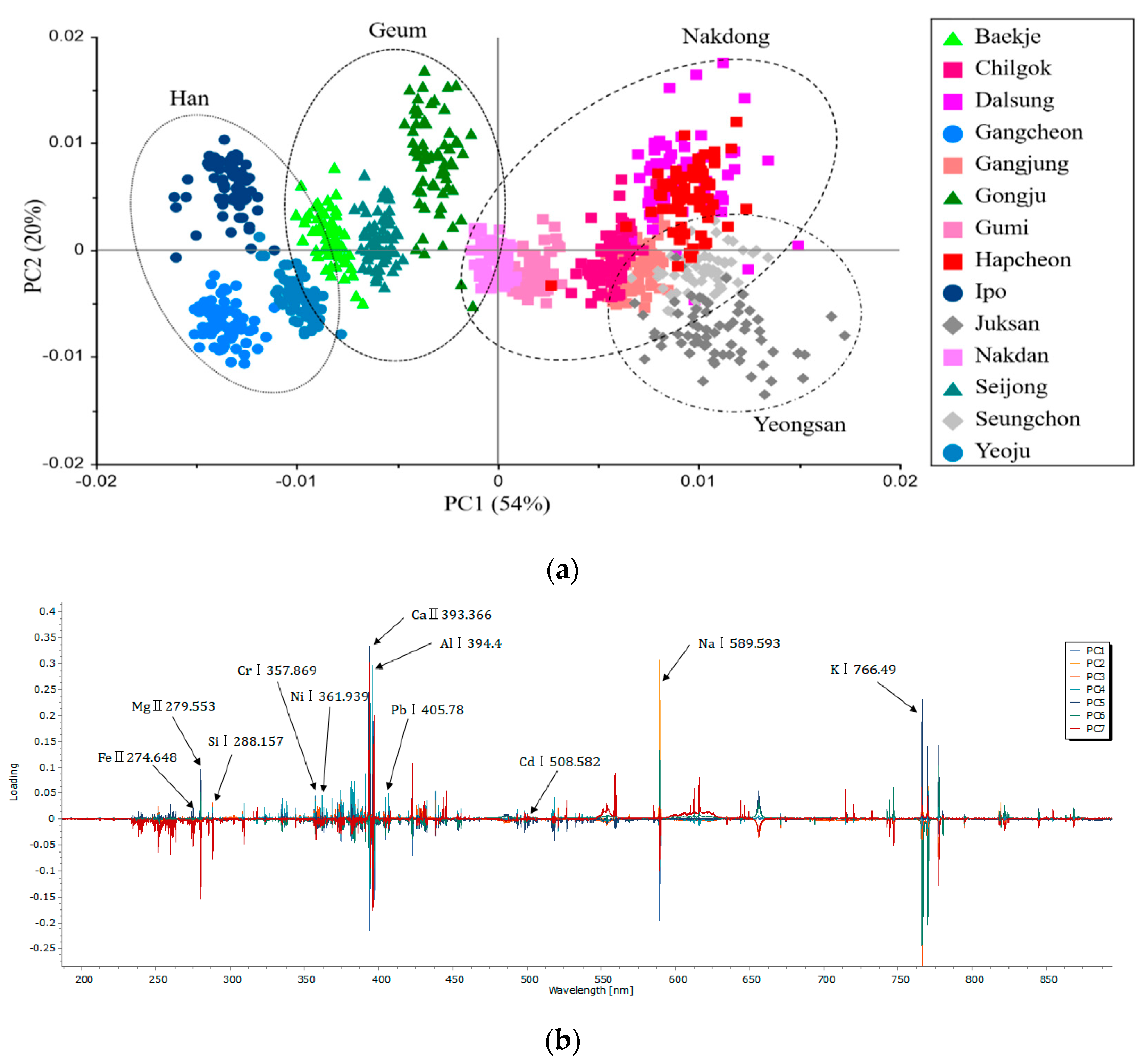
3.2. Determination and Classification of Sediment Samples

The determination and classification of the sediment samples contribute to the ability to distinguish the quality and characteristics of the sediments influencing the water quality. The quality and characteristics of the sediments depend on the differences and corresponding concentrations of the components in the sediments, which can be confirmed by the differences between the integrated spectral intensity and the wavelengths of the sediment measurements.

Before the application of PCA, area normalization, a preprocessing method, was used to scale the samples to ensure that all of the data were on approximately the same scale. The signal could be compensated for spectral changes due to matrix effects and variations in experimental conditions [12]. The classification process of the spectra could extend the calculation time and increase the performance requirements of the equipment for the LIBS measurements. Hence, the removal of undesired variables and the selection of only a few crucial emission lines were significant for the multivariate analyses.

The application of PCA transformed the full spectra into several PCs; the first seven PCs explained 90.75% of the variations in the original spectral information. Based on the score plot of the PCA, two PCs were selected as optimal PCs to explain the results of the full spectra (Figure 4a). The loading plot of the seven PCs was drawn to select the important emission lines, as shown in Figure 4b. Most of the emission lines of the main elements (Al, Ca, Cd, Cr, Fe, K, Mg, Na, Ni, Pb, and Si) exhibited relatively large loading coefficient values, which were consistent with the labeled lines for each element in Figure 4b. The emission lines with high signal-to-noise ratios were selected for further analysis. A total of 11 characteristic lines corresponding to the LIBS spectral peaks of Al, Ca, Cd, Cr, Fe, K, Mg, Na, Ni, Pb, and Si were chosen from the identified emission lines. A matrix of 896 by 11 (number of observations by lines) was then obtained to implement the subsequent analysis.

Another PCA was conducted by using the LIBS spectra at the selected characteristic lines to display any variations among the four types of sediment samples. The first two PCs explained 93.56% (PC-1: 79.21% and PC-2: 15.25%) of the variations among the total spectral results; Figure 5 shows their scores and loading plots. Each point in the scatter plot represented one spectrum. Figure 5a shows that an apparent clustering could be produced with PC-1 and PC-2. The LIBS spectra of the sediments were distinguished on the side of PC-1, whereas some spectra tended to be on the positive side of PC-2. Notably, there were distinct differences among the four groups of sediment samples.

Figure 5b shows the loading plot of the PCA, which indicated the importance of the analyzed variables. The data show that Al, Ca, and Na provided the dominant contributions to PC-1 and PC-2. To completely explain the scattering of the score plot, the loading coefficient, which is shown in Figure 5b, was utilized to analyze the scattering distribution of the four types of sediments. The Nakdong and Yeongsan classes, which had relatively high concentrations of Al and Ca, were located on the positive side of PC-1, and the Han and Geum classes, which had relatively low concentrations of Al and Ca, were located on the negative side of PC-1. In addition, the classes of Nakdong and Geum, which contained relatively high concentrations of Na, were distributed on the positive side of PC-2, and the classes of Han and Yeongsan, which had relatively low concentrations of Na, were scattered on the negative side of PC-2.

3.3. Quantitative Analysis of the Sediment Using the PLSR Model

A quantitative analysis of the metal components of sediment samples plays a significant role in the quality control and water quality management of rivers. Multivariate chemometric methods combined have recently been employed in combination with the LIBS technology in the field of soil analysis [12].

One of the multivariate chemometric methods, PLSR, was used to determine the elemental content in soil samples because it is an effective dimension-reduction method for LIBS data. Because soil is composed of various chemical components, which might increase the complexity of LIBS data [12], preprocessing of SG derivatives was employed to improve the results of the PLSR model.

Optimally performing the preprocessing for LIBS analysis can effectively reduce the noise and enhance the prediction accuracy of the PLSR model. The SG derivative is a widely used preprocessing method that can effectively eliminate noise with the appropriate selection of the derivative and smoothing parameters, such as the derivative order, polynomial degree, and number of smoothing points (NSP). It is essential to select an appropriate NSP and polynomial order in the preprocessing process. Excessive smoothing can lead to the loss of information because the emission peak lines, which contain important information, can be regarded as noise. In this study, the simple first-order derivative and second-order polynomial with five points were employed.

To determine the correlations between the samples, PLSR models were constructed by using a full cross-validation method on the averaged recorded spectra. The calibration and validation performance of the PLSR model was assessed using the R², RMSEC, and RMSECV. For an ideal model, the R² should be close to 1, whereas the RMSEC should be close to 0. Moreover, the RMSEC and RMSECV were proposed in order to assess the overall performance of the model. Lower RMSEC and RMSECV values indicate a better model quality. The number of PLS factors applied in the model presented the lowest RMSECV value. Twenty-eight analytical spectral data samples were selected to build the calibration model, and the same samples were used to test the cross-validation of the PLSR model with a leave-one-out strategy.

Table 2. The calibration and validation performance of the PLSR model.

Metal	Process	Original		SG Derivative
		R2	RMSE	R2	RMSE
Cd	Calibration	0.9963	0.0063	0.9989	0.0035
	Validation	0.9406	0.0264	0.9670	0.0197
Cr	Calibration	0.9690	7.9131	0.9736	7.3066
	Validation	0.8574	17.6165	0.8136	20.1409
Pb	Calibration	0.9718	1.2379	0.9836	0.9430
	Validation	0.6815	4.3146	0.7120	4.1029

shows the performance of the PLSR model before and after the application of preprocessing with the SG derivative for the analysis of Cd, Cr, and Pb. The results output for the Cd and Pb analysis were significantly improved with respect to the R² and RMSE from the application of the SG derivative.

For the Cd analysis, the R² values for calibration and cross-validation without the SG derivative were 0.9963 and 0.9406, respectively. The RMSE of calibration (RMSEC) and the RMSE of cross-validation (RMSECV) were 0.0063 and 0.0264, respectively. The R² and RMSE were improved with the SG derivative smoothing method. The R² values for calibration and cross-validation, the RMSEC, and the RMSECV with the SG derivative were 0.9989, 0.9670, 0.0035, and 0.0197, respectively.

For the Cr analysis, the R² values for calibration and cross-validation without the SG derivative were 0.9690 and 0.8574, respectively. The RMSEC and RMSECV were 7.91311 and 17.61650, respectively. However, the smoothing of the SG derivative did not improve the values of the R² and RMSE. The R² values for calibration and cross-validation were 0.9736 and 0.8136, respectively. The RMSEC and RMSECV decreased to 7.3066 and 20.1409, respectively.

The results of the Pb analysis showed a similar trend to those of the Cr analysis. Without the SG derivative, the R² values for calibration and cross-validation were 0.9718 and 0.6815, respectively. The RMSEC and RMSECV were 1.2379 and 4.3146, respectively. The R² and RMSE were improved with the SG derivative smoothing method. The R² values for calibration and cross-validation, the RMSEC, and the RMSECV with the SG derivative were 0.9836, 0.7120, 0.9430, and 4.1029, respectively.

In the case of Cr, the R² values for cross-validation and the RMSECV without preprocessing were better. For the cases of Cd and Pb, the R² values for cross-validation and the RMSECV were improved when the SG derivative preprocessing method was applied. To quantitatively compare the RMSEC and RMSECV for metals, the averages of the RMSEC and RMSECV were employed as follows [21]:

$$\mathrm{RMSEC}{\left(\mathrm{V}\right)}_{\mathrm{avg}}\left(\%\right)=\frac{\mathrm{RMSEC}\left(\mathrm{V}\right)}{\mathrm{Average} \mathrm{of} \mathrm{Property}}\times 100$$

(4)

The averages of the RMSECV were calculated by dividing the RMSECV by the average of the properties to quantitatively compare the RMSECV for each metal. This value allows for comparisons between the properties of samples with unequal sizes [25]. The authors of [26] used the averages of the RMSECV to find the lowest errors of different spectral features in the standard volume of forests. The authors of [27] used the averages of the RMSECV to determine the optimal model between multilinear regression and an artificial neural network for biomass.

Table 3. The averages (%) in the middle of the values (RMSEC and RMSECV).

Metal	Data Type	RMSEC Average (%)	RMSECV Average (%)
Cd	Original	2.7227	11.1519
	SG derivative	1.49018	8.35241
Cr	Original	19.5385	46.213
	SG derivative	18.0409	50.6646
Pb	Original	8.03888	27.7485
	SG derivative	6.12366	26.63

lists the averaged RMSECV values that were calculated. The results of the Cd analysis with the SG derivative show the lowest averaged RMSECV of 8.35. Although the Cd content was low in the sediment, the Cd analysis showed a somewhat higher error value. The results of the analysis of Cd showed the lowest error among the metals because Cd was in a similar concentration range. In the case of Cr, the RMSECV values were high. This can be attributed to the large deviations among the amounts of Cr contained in the samples. In terms of the averaged RMSECV, except for the Cr analysis, the application of the preprocessing with the SG derivative to the original data was conducive to the reduction of errors in the results.

The accuracy of quantitative analyses that use PLSR models can be improved by utilizing data-preprocessing techniques, such as the SG derivative. From LIBS measurements, a good amount of data can be obtained. The RSD can be too high to find a reliable correlation. Therefore, this approach will be effective in improving the ability to detect heavy metals in sediments for in situ monitoring of rivers. Furthermore, the combination of the LIBS technique with a data-processing method is expected to contribute to the provision of better interpretations and visualizations of data. From the results of this research, it was determined that the LIBS system together with multivariate chemometric analysis is useful for providing practical guidelines for the management of freshwater sediments and water quality by understanding and evaluating many potential pollutants in the sediments.

4. Conclusions

This study investigated the determination and quantification of heavy metals in river sediments using a LIBS system and multivariate chemometric analysis. Based on the characteristics of LIBS data and a PCA conducted on the full spectra, 11 characteristic lines of the main elements were identified. To simplify the discriminant model, the 11 emission lines of Al, Ca, Cd, Cr, Fe, K, Mg, Na, Ni, Pb, and Si were selected for further analysis. The PCA, which was based on the LIBS spectra at the emission lines, showed apparent clustering of four types of sediment samples, suggesting the possibility of applying this technique to discriminate different types of sediments.

PLSR models were established, and their performance was evaluated in terms of the R², RMSEC, and RMSECV. The results obtained using the PLSR with an SG derivative were improved with respect to the R² and RMSECV, except for Cr. In particular, the results for Cd obtained with the SG derivative showed a decrease of 25% in the RMSECV value. This demonstrates that the PLSR model with the SG derivative is suitable for the quantitative analysis of metal components in sediment samples. This combination can play a significant role in the quality control and water quality management of rivers.

To improve the applicability of our approach, more samples and a diversified analytical dataset should be considered to obtain sufficient spectral data in further investigations. This could provide theoretical guidance for the management of freshwater sediments and water quality.

References

1. Chen, M.; He, W.; Choi, I.; Hur, J. Tracking the monthly changes of dissolved organic matter composition in a newly constructed reservoir and its tributaries during the initial impounding period. Environ. Sci. Pollut. Res. 2016, 23, 1274–1283. [Google Scholar] [CrossRef]
2. Hur, J.; Jung, N.C.; Shin, J.K. Spectroscopic distribution of dissolved organic matter in a dam reservoir impacted by turbid storm runoff. Environ. Monit. Assess. 2007, 133, 53–67. [Google Scholar] [CrossRef]
3. Nadon, M.J.; Metcalfe, R.A.; Williams, C.J.; Somers, K.M.; Xenopoulos, M.A. Assessing the effects of dams and waterpower facilities on riverine dissolved organic matter composition. Hydrobiologia 2015, 744, 145–164. [Google Scholar] [CrossRef]
4. Yang, L.; Choi, J.H.; Hur, J. Benthic flux of dissolved organic matter from lake sediment at different redox conditions and the possible effects of biogeochemical processes. Water Res. 2014, 61, 97–107. [Google Scholar] [CrossRef]
5. Walling, D.E. Human impact on land–ocean sediment transfer by the world’s rivers. Geomorphology 2006, 79, 192–216. [Google Scholar] [CrossRef]
6. Lin, J.; Zhang, S.; Liu, D.; Yu, Z.; Zhang, L.; Cui, J.; Xie, K.; Li, T.; Fu, C. Mobility and potential risk of sediment-associated heavy metal fractions under continuous drought-rewetting cycles. Sci. Total Environ. 2018, 625, 79–86. [Google Scholar] [CrossRef] [PubMed]
7. O’Neill, F.G.; Ivanović, A. The physical impact of towed demersal fishing gears on soft sediments. ICES J. Mar. Sci. 2016, 73, i5–i14. [Google Scholar] [CrossRef] [Green Version]
8. Yi, Y.; Yang, Z.; Zhang, S. Ecological risk assessment of heavy metals in sediment and human health risk assessment of heavy metals in fishes in the middle and lower reaches of the Yangtze River basin. Environ. Pollut. 2011, 159, 2575–2585. [Google Scholar] [CrossRef] [PubMed]
9. Michel, A.P.M.; Sonnichsen, F. Laser induced breakdown spectroscopy for heavy metal detection in a sand matrix. Spectrochim. Acta Part B At. Spectrosc. 2016, 125, 177–183. [Google Scholar] [CrossRef] [Green Version]
10. Capitelli, F.; Colao, F.; Provenzano, M.R.; Fantoni, R.; Brunetti, G.; Senesi, N. Determination of heavy metals in soils by laser induced breakdown spectroscopy. Geoderma 2002, 106, 45–62. [Google Scholar] [CrossRef]
11. Senesi, G.S.; Dell’Aglio, M.; Gaudiuso, R.; De Giacomo, A.; Zaccone, C.; De Pascale, O.; Miano, T.M.; Capitelli, M. Heavy metal concentrations in soils as determined by laser-induced breakdown spectroscopy (LIBS), with special emphasis on chromium. Environ. Res. 2009, 109, 413–420. [Google Scholar] [CrossRef]
12. Yu, K.Q.; Zhao, Y.R.; Liu, F.; He, Y. Laser-induced breakdown spectroscopy coupled with multivariate chemometrics for variety discrimination of soil. Sci. Rep. 2016, 6, 27574. [Google Scholar] [CrossRef]
13. Kim, G.; Kwak, J.; Kim, K.R.; Lee, H.; Kim, K.W.; Yang, H.; Park, K. Rapid detection of soils contaminated with heavy metals and oils by laser induced breakdown spectroscopy (LIBS). J. Hazard. Mater. 2013, 263, 754–760. [Google Scholar] [CrossRef] [PubMed]
14. Lal, B.; Zheng, H.; Yueh, F.-Y.; Singh, J.P. Parametric study of pellets for elemental analysis with laser-induced breakdown spectroscopy. Appl. Opt. 2004, 43, 2792–2797. [Google Scholar] [CrossRef] [PubMed]
15. Noll, R. Laser-Induced Breakdown Spectroscopy: Fundamentals and Applications, 1st ed.; Springer: Berlin, Germany, 2012. [Google Scholar]
16. Anzano, J.; Bonilla, B.; Montull-Ibor, B.; Casas-González, J. Plastic identification and comparison by multivariate techniques with laser-induced breakdown spectroscopy. J. Appl. Polym. Sci. 2011, 121, 2710–2716. [Google Scholar] [CrossRef]
17. Tuukkanen, T.; Marttila, H.; Kløve, B. Predicting organic matter, nitrogen, and phosphorus concentrations in runoff from peat extraction sites using partial least squares regression. Water Resour. Res. 2017, 53, 5860–5876. [Google Scholar] [CrossRef]
18. Stellacci, A.M.; Castellini, M.; Diacono, M.; Rossi, R.; Gattullo, C.E. Assessment of soil quality under different soil management strategies: Combined use of statistical approaches to select the most informative soil physico-chemical indicators. Appl. Sci. 2021, 11, 5099. [Google Scholar]
19. Tsai, F.; Philpot, W. Derivative analysis of hyperspectral data. Remote Sens. Environ. 1998, 66, 41–51. [Google Scholar] [CrossRef]
20. Filzmoser, P.; Liebmann, B.; Varmuza, K. Repeated double cross validation. J. Chemom. 2009, 23, 160–171. [Google Scholar] [CrossRef]
21. Nagelkerke, N.J.D. A note on a general definition of the coefficient of determination. Biometrika 1991, 78, 691–692. [Google Scholar] [CrossRef]
22. Willmott, C.J.; Matsuura, K. Advantages of the mean absolute error (MAE) over the root mean square error (RMSE) in assessing average model performance. Clim. Res. 2005, 30, 79–82. [Google Scholar] [CrossRef]
23. Gondal, M.A.; Hussain, T.; Yamani, Z.H.; Baig, M.A. The role of various binding materials for trace elemental analysis of powder samples using laser-induced breakdown spectroscopy. Talanta 2007, 72, 642–649. [Google Scholar] [CrossRef] [PubMed]
24. Chen, H.; Song, Q.; Tang, G.; Feng, Q.; Lin, L. The combined optimization of Savitzky-Golay smoothing and multiplicative scatter correction for FT-NIR PLS models. ISRN Spectrosc. 2013, 2013, 642190. [Google Scholar] [CrossRef] [Green Version]
25. Li, L. Partial least squares modeling to quantify lunar soil composition with hyperspectral reflectance measurements. J. Geophys. Res. E Planets. 2006, 111, e04002. [Google Scholar] [CrossRef] [Green Version]
26. Mäkelä, H.; Pekkarinen, A. Estimation of forest stand volumes by Landsat TM imagery and stand-level field-inventory data. For. Ecol. Manage. 2004, 196, 245–255. [Google Scholar] [CrossRef]
27. Xie, Y.; Sha, Z.; Yu, M.; Bai, Y.; Zhang, L. A comparison of two models with Landsat data for estimating above ground grassland biomass in Inner Mongolia, China. Ecol. Modell. 2009, 220, 1810–1818. [Google Scholar] [CrossRef]
Figure 1. Study site.
Applsci 11 07154 g001
Figure 2. Main emission lines of the target elements (Cd, Cr, Pb) in the LIBS spectra of the sediment samples.
Applsci 11 07154 g002
Figure 3. RSD results with an increasing starch-mixing ratio: (a) Cd at 361.051 nm, (b) Cr at 274.898 nm, and (c) Pb at 537.210 nm.
Applsci 11 07154 g003
Figure 4. Score plot of the first two PCs (a) and loading plot of the seven PCs (b); the plots of the seven PCs from the PCA use the full spectra of the sediment samples.
Applsci 11 07154 g004
Figure 5. Score (a) and loading (b) plots of first two PCs from the PCA on the LIBS spectra at the selected lines of sediment samples.
Applsci 11 07154 g005