Numerical Parametric Study on the Effectiveness of the Contact-Point Response of a Stationary Vehicle for Bridge Health Monitoring

Abstract

Indirect bridge health monitoring is conducted by running an instrumented vehicle over a bridge, where the vehicle serves as a source of excitation and as a signal receiver; however, it is also important to investigate the response of the instrumented vehicle while it is in a stationary position while the bridge is excited by other source of excitation. In this paper, a numerical model of a stationary vehicle parked on a bridge excited by another moving vehicle is developed. Both stationary and moving vehicles are modeled as spring–mass single-degree-of-freedom systems. The bridges are simply supported and are modeled as 1D beam elements. It is known that the stationary vehicle response is different from the true bridge response at the same location. This paper investigates the effectiveness of contact-point response in reflecting the true response of the bridge. The stationary vehicle response is obtained from the numerical model, and its contact-point response is calculated by MATLAB. The contact-point response of the stationary vehicle is investigated under various conditions. These conditions include different vehicle frequencies, damped and undamped conditions, different locations of the stationary vehicle, road roughness effects, different moving vehicle speeds and masses, and a longer span for the bridge. In the time domain, the discrepancy of the stationary vehicle response with the true bridge response is clear, while the contact-point response agrees well with the true bridge response. The contact-point response could detect the first, second, and third modes of frequency clearly, unlike the stationary vehicle response spectra.

1. Introduction

The structural deterioration of bridges could pose life-threatening risks to crossing pedestrians, vehicles, and trains. Consequently, health assessment and monitoring of bridges is of great interest to both authorities and stakeholders. The deterioration of bridges could occur due to flooding, earthquakes, winds, or repeated passing loads. The need to establish efficient methods to monitor bridges is increasing as aging structures have higher possibilities of damage occurrence [1,2]. In Europe, for example, most bridges were constructed in the post-War era between 1945 and 1965 [3]. In Japan, almost one-third of bridges have been in service for over 50 years [4]. In the United States, there are more than 66,000 structurally deficient bridges which account for 11% of total bridges, and most of the bridges in total are older than 65 years old [5].

Bridge health monitoring refers to the identification of dynamic modal characteristics and damage detection in bridges. Dynamic modal characteristics such as frequency, damping, and mode shapes reflect the physical properties of the structure and can be used in models to assess the health state of the structure. On the other hand, damage detection includes the identification of the existence, location, and severity of damage and, finally, the life expectancy of the structure [6,7,8]. It is important to note that the modal properties used for the identification and detection of damage in bridges are influenced by environmental factors such as temperature, which necessitates extensive work to study bridge response under varying temperatures [9,10].

Direct vibration-based bridge health monitoring is performed by installing a large number of sensors directly on the bridge to record bridge vibrations. Then, the vibration signals are processed to estimate the health state of the bridge [11,12]; however, it is difficult to implement a direct method on a wide scale for several reasons. First, such a sensory system bears a high cost for equipment and installation. Second, the life expectancy of the sensory system is shorter than that of the bridge itself, so regular maintenance of the system is required. Third, installation could be dangerous for many types of bridges. Fourth, due to limitations regarding sensor locations, accelerometers may not be able to detect remote damage [13,14].

In 2004, Yang and Lin [15] proposed an indirect vibration-based approach to overcome the issues of direct methods. Their approach employed an instrumented vehicle to record vibration signals while passing over a bridge. The recorded vibrations are then processed in order to assess the health state of the bridge. This indirect method is especially cost effective because it requires one or few sensors to be installed on a vehicle. The sensors could be installed on a typical vehicle [16], or on a special trailer attached to a vehicle [12]. This indirect method is highly mobile because the instrumented vehicle can be used for an unlimited number of bridges. Besides, the passing vehicle scans the vibration of every point of the bridge, unlike the direct method, which is limited to the locations of the sensors. The feasibility of the indirect method has been proven by field test experiments when Lin and Yang [17] extracted the fundamental frequency of a real bridge from a passing vehicle.

Since then, the indirect method has attracted the attention of many researchers who are interested in bridge health monitoring. Several techniques have been proposed to obtain higher accuracy and extract higher modes of frequencies when using a scanning vehicle [18,19,20]. Also, several methods have been proposed to construct mode shapes for bridges when considering a passing vehicle [21,22,23]. Damage detection employing the indirect method has been conducted using several approaches such as wavelet transformation, empirical mode decomposition, and Hilbert–Huang transformation [24,25,26,27]. Field tests and laboratory experiments have been conducted to identify modal properties and detect bridge damage [28,29,30,31]. Despite the great efforts that have been accomplished, the pollution of recorded signals is still an obstacle to implementing an indirect method [13]. This corruption of signals may occur due to the vehicle’s own vibration frequency or due to road irregularities.

One of the recent methods proposed to obtain more accurate results from a scanning vehicle is the contact-point response calculation approach which was proposed by Yang and Zhang [32]. The contact point refers to the point on the underside of the vehicle tire which is in direct contact with the bridge. The accelerometer mounted on the vehicle measures the vertical vibration of the vehicle during its passage over the bridge; however, this response is distorted by the vehicle frequency, which corrupts the acceleration signal. As such, it is more accurate to use the contact-point response instead of the vehicle response. Contact-point response has the advantage of being free of the vehicle frequency which may overshadow the bridge frequency. Yang and Zhang [32] proposed a method to calculate the contact-point response of the moving vehicle. The contact-point response of a moving vehicle has exhibited promising results for crack identification when performing numerical simulation for a bridge model [33,34]. The scanning vehicle can be used in moving or stationary conditions. Previous work has been carried out for a moving vehicle and this paper instead addresses the contact-point response for a stationary vehicle when a bridge is excited by a moving vehicle.

Recently, Li and Zhu [35] proposed an approach which utilized the response of a stationary vehicle to overcome the issue of road roughness; however, in their study, the stationary vehicle response does not reflect the true vibration of the bridge because the stationary vehicle response is distorted by its own frequency. Few studies have been dedicated to the analysis of stationary vehicle vibration due to excitation from moving vehicles. Oshima and Yamamoto [36] and He and Ren [37] employed stationary vehicle responses for bridge damage identification; however, they considered the stationary vehicle as a lumped mass, which is not realistic. Lin and Yang [17] demonstrated how the response of a stationary vehicle is different from the true response of the bridge in a field test experiment. He and Ren [38] employed stationary vehicle vibration for mode shape identification in bridges; however, their bridge was excited by ambient vibrations, such as wind. Very recently, Yang and Xu [39] compared the response of a moving vehicle and a stationary vehicle (the vehicle in a non-moving state) in a field experiment. They found that the response of the stationary vehicle could detect more bridge frequencies than the moving vehicle; however, they used an arbitrary source of excitation to excite the stationary vehicle, such as people jumping on the bridge. Also, they only considered one location in the bridge’s span.

The numerical investigations that have been carried out on the vibration of a stationary vehicle over a bridge still lack several aspects, such as the effects of the vehicle’s frequency, damping effects, stationary vehicle’s location, and road roughness effects. Also, the properties of the source of excitation (moving vehicle), such as the speed and mass, have not been discussed by previous studies. As such, more research is required to confirm the behavior of a stationary vehicle when parked on a bridge. This study is dedicated to investigating the response of a stationary vehicle and the contact-point response via the use of a finite element (FE) model of the stationary vehicle when parked on a bridge that is traversed by a moving vehicle. First, a vehicle bridge interaction formulation is presented and used to validate the FE model. Then, the response of the stationary vehicle is obtained from the FE model. The contact-point response is calculated by MATLAB and compared with the true bridge response. Several factors are investigated, such as different vehicle frequencies, damped and undamped conditions, different locations of the stationary vehicle, and different moving vehicle speeds and masses.

2. Analytical Programming

2.1. Formulation of Bridge Dynamic Response

This section elaborates on how the dynamic responses of bridges are derived analytically. These analytical formulations are important to understanding the key parameters influencing bridge vibration in the case of a moving vehicle. Also, the formulations will be used in this study to verify the adopted FE model. The closed-form formulations of the displacement and acceleration responses of the bridge may be obtained for the vehicle bridge interaction (VBI) problem shown in Figure 1 [40].

The equation of motion for an undamped simply supported beam traversed by a moving load is expressed as follows:

$$m\ddot{u}+EI{u}^{″″}=P(t)$$

(1)

where m and EI are the mass per unit length and flexural stiffness of the bridge, respectively; u is the displacement response of the bridge, where the dot (${}^{•}$) denotes differentiation with respect to time and the dash (${}^{\prime }$) denotes differentiation with respect to location; P(t) is the contact force of the moving load. The deflection of the bridge at the mid-span location can be written in a general form for all modes of vibration for a simply supported beam as follows:

$$u(\mathrm{x},\mathrm{t})=q_n(t)\sin \left(\frac{n\pi x}{L}\right)$$

(2)

where $q_n$ is the generalized coordinate; $n$ is the mode number; $x$ is the location on the bridge; and $L$ is the total length of the bridge. By differentiating Equation (2) with respect to time and location and substituting the results into Equation (1), then multiplying both sides of the equation by $\sin \left(n\pi x/L\right)$ and integrating with respect to the length $L$, one may obtain the following:

$${\ddot{q}}_n+{\omega }_{bn}^2{q}_n=\frac{-2m_{v}g}{mL}\sin {\omega }_{dn}t$$

(3)

where m_v and v are the mass and velocity of the moving load, respectively. ${\omega }_{dn}$ is the driving frequency of the moving load of the nth mode and is expressed such that ${\omega }_{dn}=\frac{n\pi v}{L}$, where ${\omega }_{bn}^{}$ is the bridge’s natural frequency for the nth mode and can be calculated as follows:

$${\omega }_{bn}=\frac{n^2{\pi }^2}{L^2}\sqrt{\frac{EI}{m}}$$

(4)

Equation (3) is solved as a differential equation using the zero initial conditions to provide the following equation:

$$q_n(t)=\frac{{\Delta }_{stn}}{1-S_n^2}\left(\sin {\omega }_{dn}t-S_n\sin {\omega }_{bn}t\right)$$

(5)

where the constant ${\Delta }_{stn}$ is expressed as ${\Delta }_{stn}=-\frac{2m_{v}g{L}^3}{EI{n}^4{\pi }^4}$ and S_n is called the speed parameter and is presented as $S_n=\frac{{\omega }_{dn}}{{\omega }_{bn}}$. The displacement response of the bridge for all modes is obtained by substituting Equation (5) into Equation (2), which is shown in Equation (6). The velocity response is obtained by differentiating the displacement as shown in Equation (7), and the acceleration response is obtained by differentiating the displacement response twice with respect to time, as shown in Equation (8).

$$u(\mathrm{x},\mathrm{t})={\displaystyle \sum _n\frac{{\Delta }_{stn}}{1-S_n^2}\sin \left(\frac{n\pi x}{L}\right)\left(\sin {\omega }_{dn}t-S_n\sin {\omega }_{bn}t\right)}$$

(6)

$$\dot{u}(\mathrm{x},\mathrm{t})={\displaystyle \sum _n\frac{{\Delta }_{stn}}{1-S_n^2}\sin \left(\frac{n\pi x}{L}\right)\left({\omega }_{dn}\cos {\omega }_{dn}t-S_n{\omega }_{bn}\cos {\omega }_{bn}t\right)}$$

(7)

$$\ddot{u}(\mathrm{x},\mathrm{t})={\displaystyle \sum _n\frac{{\Delta }_{stn}}{1-S_n^2}\sin \left(\frac{n\pi x}{L}\right)\left(-{\omega }_{dn}^2\sin {\omega }_{dn}t+S_n{\omega }_{bn}^2\sin {\omega }_{bn}t\right)}$$

(8)

The displacement, velocity, and acceleration responses, considering all modes of vibration of a simply supported beam, may be obtained analytically by the preceding equations. The equations show that bridge vibration is dominated by two frequencies, i.e., the driving frequency and bridge frequency. In this study, the responses obtained from the analytical solution are compared with those of the developed FE model to verify the prepared FE model.

2.2. Finite Element Modeling

In the previous section, the response of the bridge at mid-span location was elaborated upon analytically; however, the analytical solution does not cover complicated cases such as the vibration of a stationary vehicle parked on a bridge while another vehicle is running over the bridge. For such a complicated case, a FE method may be implemented. A FE model was created to represent stationary vehicle vibration due to excitation from a moving vehicle on a bridge as shown in Figure 2.

The bridge, moving vehicle, and stationary vehicle were modeled using the finite element program LS-DYNA as shown in Figure 3. The stationary vehicle was modeled as a single-degree-of-freedom spring–mass system as recommended by Yang et al. [15]. The FE model response of the lumped mass of the stationary vehicle represents the response recorded by an accelerometer installed on a parked vehicle in practice. The moving vehicle was also modeled as a spring–mass system, which in practice represents a truck moving over the bridge as a source of excitation. Discrete spring elements were used with the S01-SPRING_ELASTIC material model. The bridge was simply supported and made of Belytschko–Schwer beam elements with an elastic material model (MAT_001). The FE bridge response at the mid-span location represents the response of a fixed sensor mounted at the mid-span location of a real-life bridge. The stationary vehicle was attached to the bridge by means of merging the nodes at the contact point while the interaction between the bridge and the moving vehicle was modeled using RAIL_TRACK/TRAIN. The output sampling frequency was 200 Hz.

The bridge parameters in this study were adopted from the study of Yang et al. [15]. The bridge is a steel bridge with one span that is 25 m length. The elastic modulus of the bridge is 27.5 GN/m², the moment of inertia is 0.12 m⁴, and mass per unit length is 4800 kg/m. For the moving vehicle, the mass is 1200 kg, the spring stiffness is 500 kN/m (except for the case when different mass is investigated). Also, the speed of the moving vehicle is 10 m/s (expect for the case when different speed is investigated), as will be shown in the parametric case study in Section 3. The first four bridge frequencies obtained from the FE eigenvalue analysis were 2.08 Hz, 8.30 Hz, 18.59 Hz, and 32.82 Hz. The stationary vehicle in this study represents a cart parked at a bridge. The properties of the stationary vehicle such as mass and stiffness are assigned according the case to be studied in the parametric study in Section 3.

2.3. FE Model Verification

The developed FE model of a bridge traversed by a moving vehicle is verified in this section. First, eigenvalue analysis was conducted on the FE bridge model to obtain the natural frequencies of the bridge. The frequencies obtained from the FE eigenvalue analysis were compared with the calculated frequencies using Equation (4) as shown in

Table 1. Bridge eigenvalues obtained from the FE model and analytical formulation.

Mode	Frequency (Hz)
	FE Model (Ls-Dyna)	Analytical (Equation (4))
1st	2.082	2.084
2nd	8.303	8.335
3rd	18.589	18.755
4th	32.817	33.342

.

The displacement and acceleration responses of the FE bridge model due to the moving vehicle were also verified by the analytical formulations by employing Equations (6)–(8). Figure 4 shows the displacement, velocity, and acceleration responses obtained by the FE model and analytical solution. The small deviation which occurs after the vehicle passes the mid-span is insignificant and negligible. The good agreement between the FE model and analytical solution results proves the validity of the developed FE model.

2.4. Contact-Point Response

In practical applications, only the acceleration response from the accelerometer installed on the stationary vehicle is available, such as ${\ddot{q}}_s$. Although it has been proven that the vehicle response (${\ddot{q}}_s$) contains the bridge frequency, it is clear that such a response also contains the vehicle’s own frequency; however, the contact-point response (${\ddot{u}}_c$) is free from the vehicle frequency, which could provide the bridge’s true response at the location of the parked vehicle. This section elaborates on the process of how the contact-point response is calculated. The equation of motion for the stationary vehicle is expressed as follows:

$$m_s{\ddot{q}}_s+k_s\left(q_s-u_c\right)=0$$

(9)

where $m_s$ and $k_s$ are the mass and stiffness of the stationary vehicle, respectively. Deriving the equation of motion for the stationary vehicle twice with respect to time could yield the following:

$$-k_s\left({\ddot{q}}_s-{\ddot{u}}_c\right)=m_s\frac{d^2{\ddot{q}}_s}{d{t}^2}$$

(10)

The natural frequency of the stationary vehicle is known in practice and can be expressed as ${\omega }_s=\sqrt{k_s/m_s}$. Consequently, the contact-point acceleration of the stationary vehicle can be computed as follows:

$${\ddot{u}}_c={\ddot{q}}_s+\frac{d^2{\ddot{q}}_s}{{\omega }_s^{2}d{t}^2}$$

(11)

The term $\frac{d^2{\ddot{q}}_s}{d{t}^2}$ can be calculated by the central difference method for the discrete data of the recorded signal such that

$$\frac{d^2{\ddot{q}}_s}{d{t}^2}=\frac{\left({\ddot{q}}_s{|}_{i+1}-2{\ddot{q}}_s{|}_i+{\ddot{q}}_s{|}_{i-1}\right)}{{(\Delta t)}^2},$$

(12)

where $\Delta t$ denotes the sampling interval and $i$ is the $ith$ sampling point. In this study, the vertical acceleration of the stationary vehicle obtained from the FE model was used to calculate the contact-point response. Afterwards, the contact-point response was compared to the true response of the bridge to check the efficiency of the proposed approach.

3. Parametric Study

In this section, numerical simulations are employed to view the capability of the contact-point response of a stationary vehicle to present the true vibration of a bridge. Key parameters affecting the stationary vehicle and its contact-point responses were investigated. The first part of this section discusses the reliability of the contact-point response for various stationary vehicle frequencies. The second part investigates the effects of damping on the stationary vehicle response and its contact-point response. The third part investigates the location of the stationary vehicle. The fourth part investigates the effects of the road roughness on the response of the stationary vehicle and its contact-point response. The fifth and sixth parts investigate the different properties of the moving vehicle, such as the speed and mass. Finally, the response of a stationary vehicle and its contact-point response are investigated for a bridge with a long span.

The investigations were conducted considering three responses, i.e., the stationary vehicle response, the true bridge response, and the contact-point response. The stationary vehicle response was obtained from the upper node of the spring–mass vehicle that was parked at the bridge in the FE model. The true bridge response (reference response) was obtained from the node located at the same location of the stationary vehicle. The contact-point response of the stationary vehicle was calculated in MATLAB using Equations (11) and (12) and by employing the stationary vehicle response. The true bridge response was used to judge to what extent the stationary vehicle response and contact-point response could reflect the true bridge response. Comparisons between the true bridge response, stationary vehicle response, and contact-point response are presented for each case study. The comparisons are made in the time domain to expose the differences in amplitude and phase change in the acceleration signals. The comparisons are also made in the frequency domain to identify the ability of the signal to detect bridge frequencies. As such, a fast Fourier transform (FFT) was used with each acceleration signal.

3.1. Effect of Stationary Vehicle Frequency

The physical properties of the instrumented vehicle, such as the mass and stiffness, play a crucial role in indirect bridge dynamic response identification. This section discusses four stationary vehicle different cases with a different frequency for each case. The contact-point response of vehicles having lower, similar, or higher frequencies than the fundamental frequency of the bridge are discussed. The mass of the stationary vehicle remained unchanged throughout all cases while the stiffness was altered to have different frequencies.

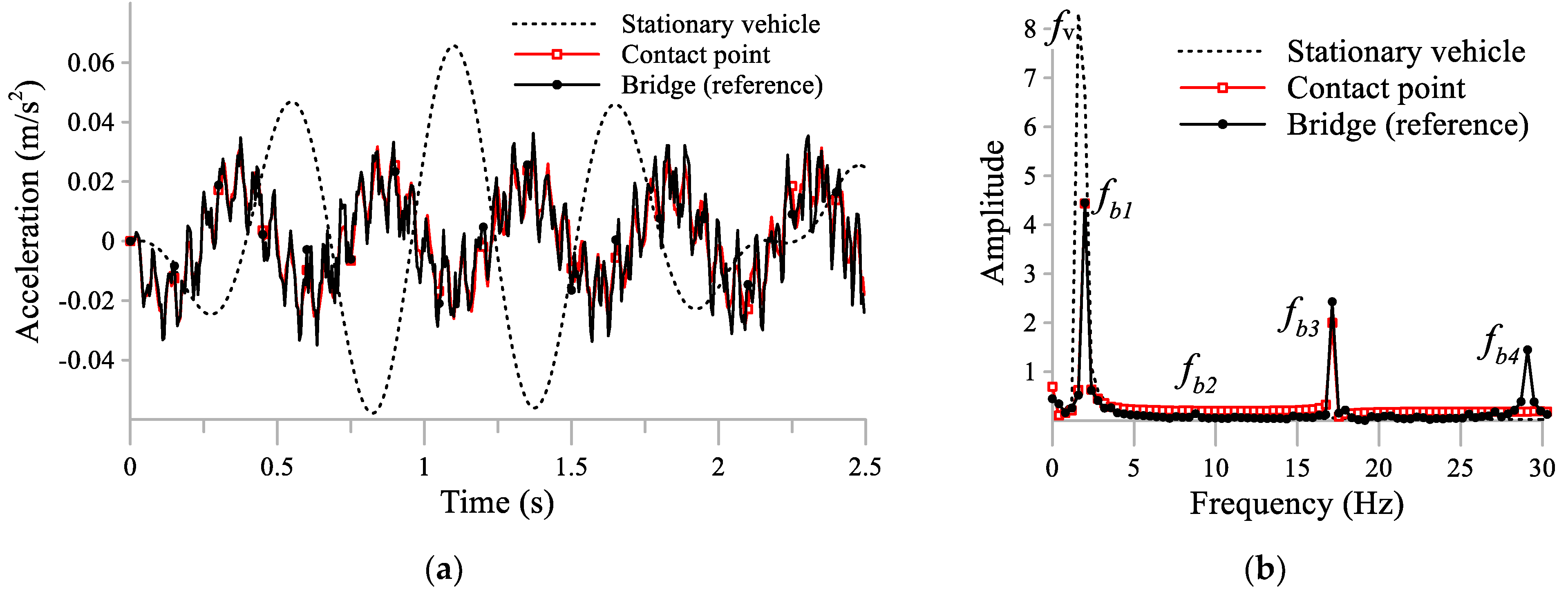
3.1.1. Vehicle Frequency Lower Than any Bridge Frequency

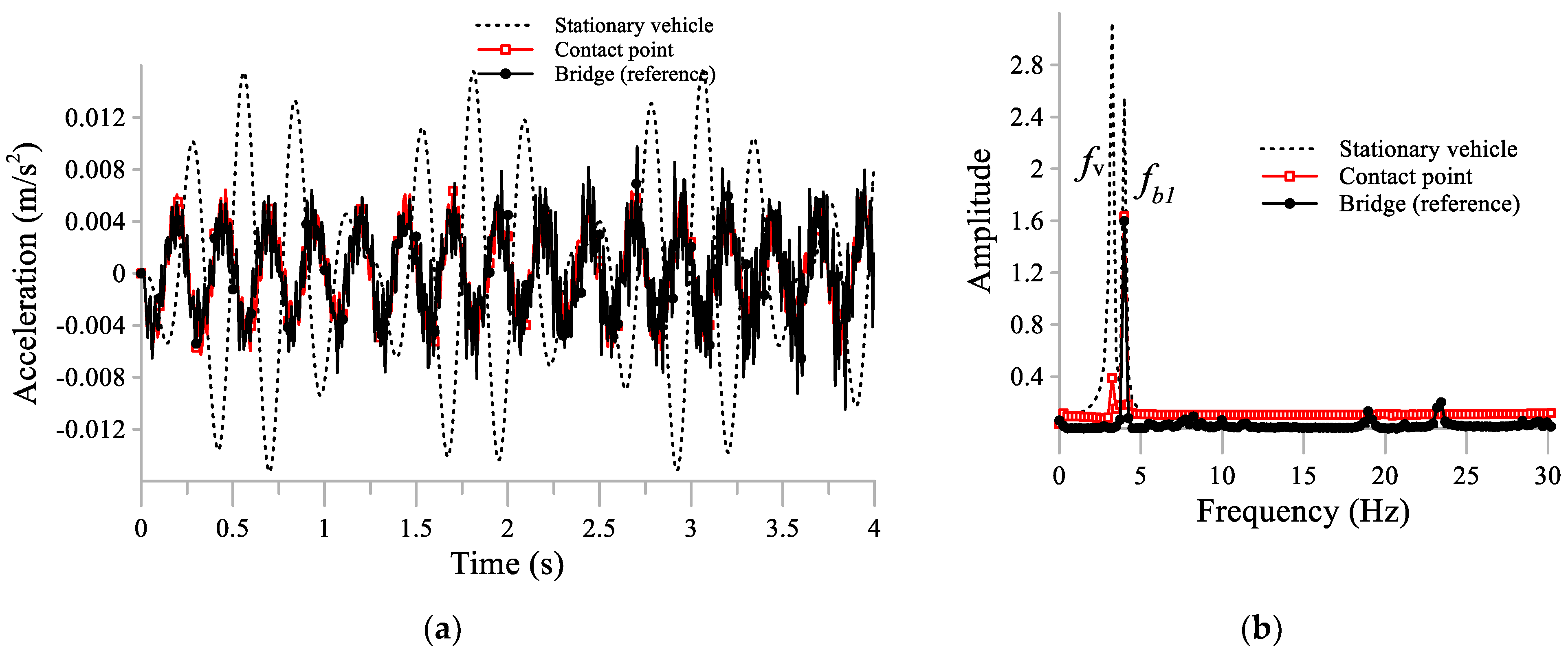
The first case considers a stationary vehicle with a vertical frequency of 1.59 Hz, which is less than the bridge’s first frequency of 2.08 Hz. The mass of the stationary vehicle was 200 kg and the simulation stiffness was 20,000 N/m. The moving vehicle properties were as mentioned earlier with a speed of 10 m/s and frequency of 3.25 Hz. The true bridge response, stationary vehicle response, and its contact-point response are shown in Figure 5a. The stationary vehicle response is very smooth, which implies that it does not contain higher modes of vibration. On the other hand, the contact-point response is in good agreement with the bridge vibration. Figure 5b shows the FFT of the acceleration response of the bridge, contact-point, and stationary vehicle. The stationary vehicle acceleration spectrum does not clearly show the fundamental bridge frequency of 2.08 Hz. Higher modes of vibration do not even exist in the stationary vehicle response; however, the contact-point acceleration spectrum shows the fundamental bridge frequency clearly and shows the third mode of vibration. The second mode of vibration at 8.33 Hz is barely visible in the bridge response spectrum as shown in Figure 5b. That occurs because the second mode shape of a simply supported bridge is zero at the mid-span location. When the stationary vehicle is located at other locations, for example, at the quarter-span location, the second mode will be visible as will be demonstrated in Section 3.3. Finally, the fourth mode of frequency is visible in the bridge response but it is not detected by the contact-point response. This trend occurs for all cases as will be shown below. This occurs due to the numerical inaccuracies that are produced when numerically calculating the second derivative of the stationary vehicle’s acceleration response. It is important to note that the frequency of the stationary vehicle is almost eliminated in the contact-point response. Furthermore, it is not completely eliminated due to numerical derivation inaccuracy.

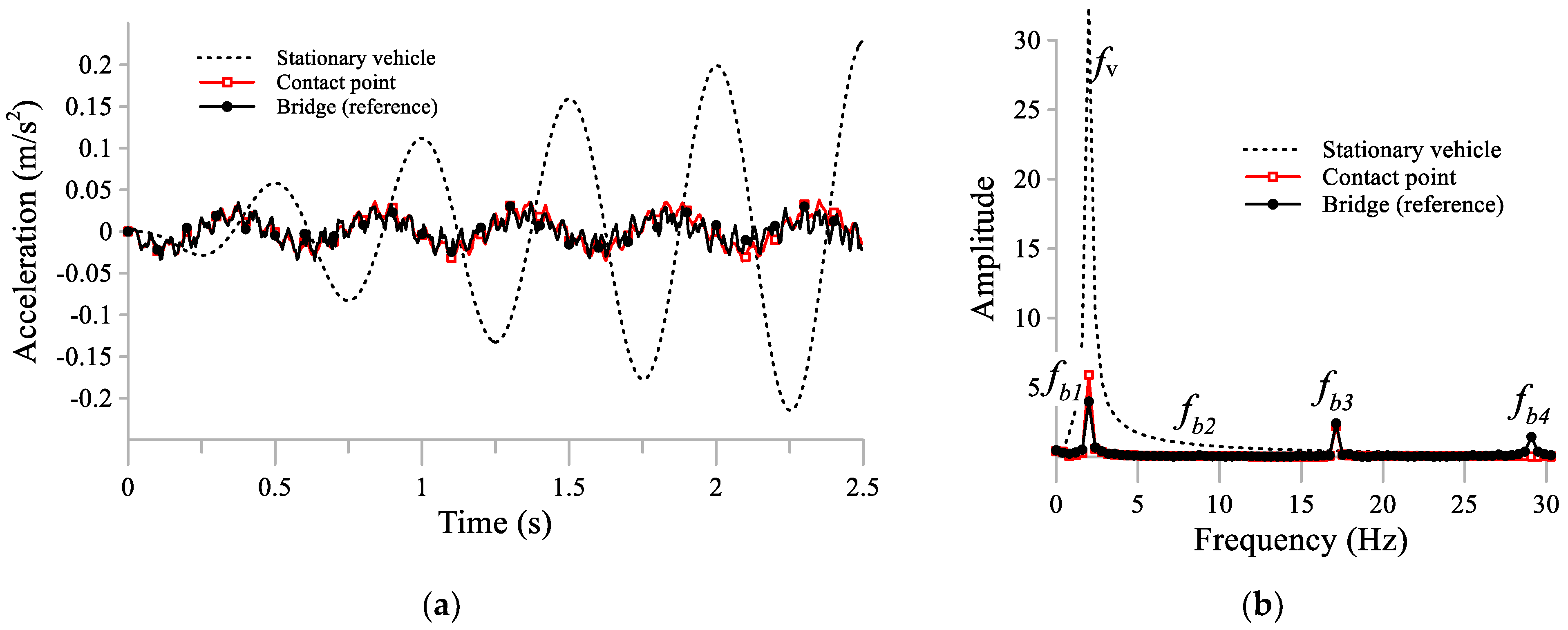
3.1.2. Vehicle Frequency Close to the Bridge’s Fundamental Frequency (Resonance Case)

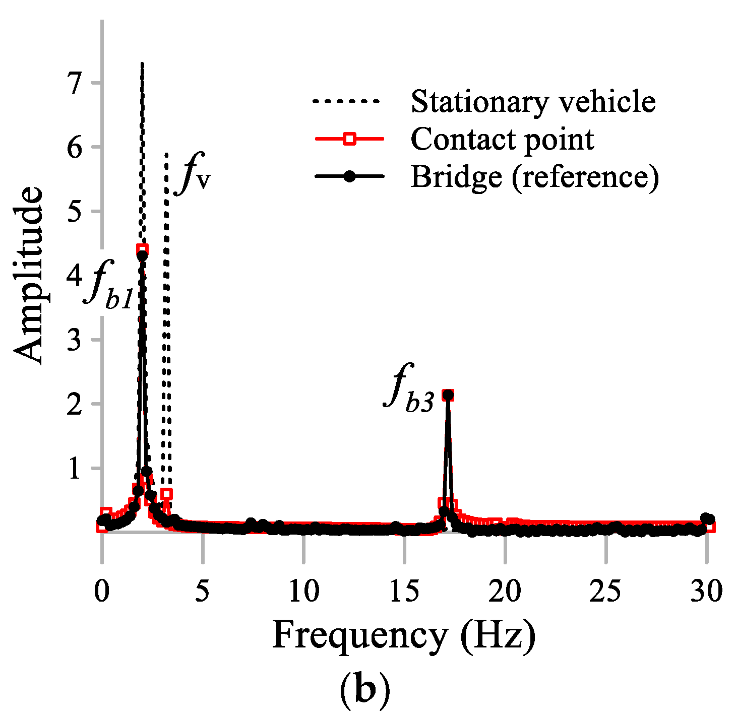
To show the contact-point response reliability in the case of resonance, a stationary vehicle with a frequency of 1.95 Hz was selected. The vehicle stiffness was 30,000 N/m and the mass was 200 kg. The stationary vehicle frequency was very close to the bridge fundamental frequency of 2.08 Hz. The speed and properties of the moving vehicle remained unchanged from the previous case. Although the stationary vehicle response was vastly amplified, its contact-point response agreed well with the true bridge response, as shown in the acceleration responses in Figure 6a. The acceleration response spectra in Figure 6b also show good agreement between the bridge and contact-point responses; however, there was a small but noticeable difference between the bridge and contact-point response spectra in the amplitude of the first frequency mode. This difference only occurred in the case of resonance, unlike the other cases where the stationary vehicle frequency is far from the bridge’s fundamental frequency. The stationary vehicle acceleration spectrum showed only one frequency at 2 Hz, which was the frequency of both the bridge and the vehicle. In contrast, the contact-point response spectrum shows the third mode frequency of the bridge at around 18 Hz.

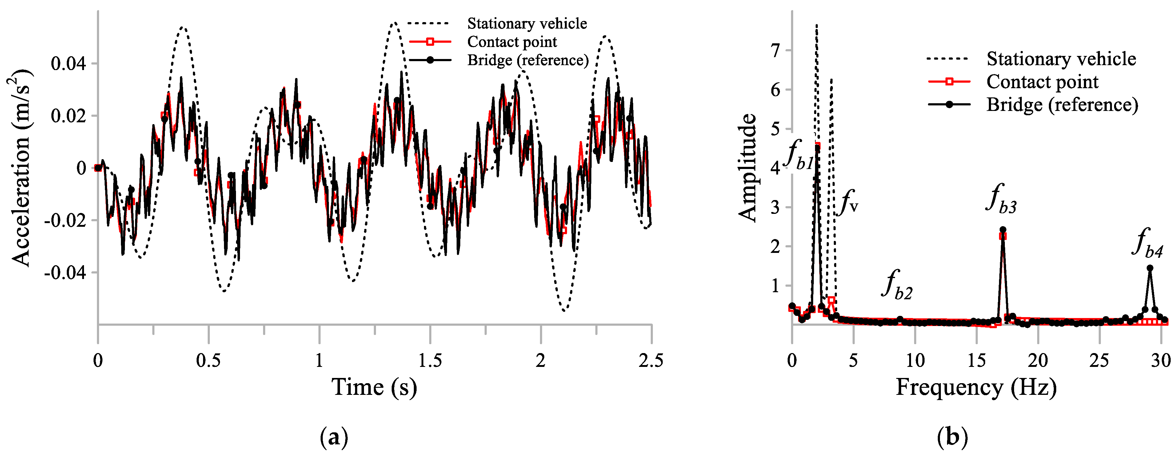
3.1.3. Vehicle Frequency Higher Than Bridge’s Fundamental Frequency

The third case considered a stationary vehicle with a frequency of 3.18 Hz, which is slightly higher than the bridge’s fundamental frequency. The mass of the vehicle remained at 200 kg, but the stiffness was increased to be 80,000 N/m. It is important to note that the stationary vehicle properties in this case, such as mass and stiffness, will be used in Section 3.2, Section 3.3, Section 3.4, Section 3.5, Section 3.6 and Section 3.7.

The stationary vehicle, contact-point, and bridge responses are shown in Figure 7a, and the acceleration spectra are shown in Figure 7b. Similar to the previous cases, the stationary vehicle response did not contain higher modes of vibration and the contact-point response was in good agreement with the bridge response. Unlike the 1.6-Hz stationary vehicle, the 3.18-Hz stationary vehicle response could detect the first mode of frequency of the bridge. Meanwhile, it is clear that the stationary signal was corrupted by its own frequency, which appears as the second peak in Figure 7b. This led to difficulties in identifying damage on the bridge because the signal was polluted by the vehicle frequency. Nevertheless, the frequency of the stationary vehicle was almost eliminated for the contact-point response.

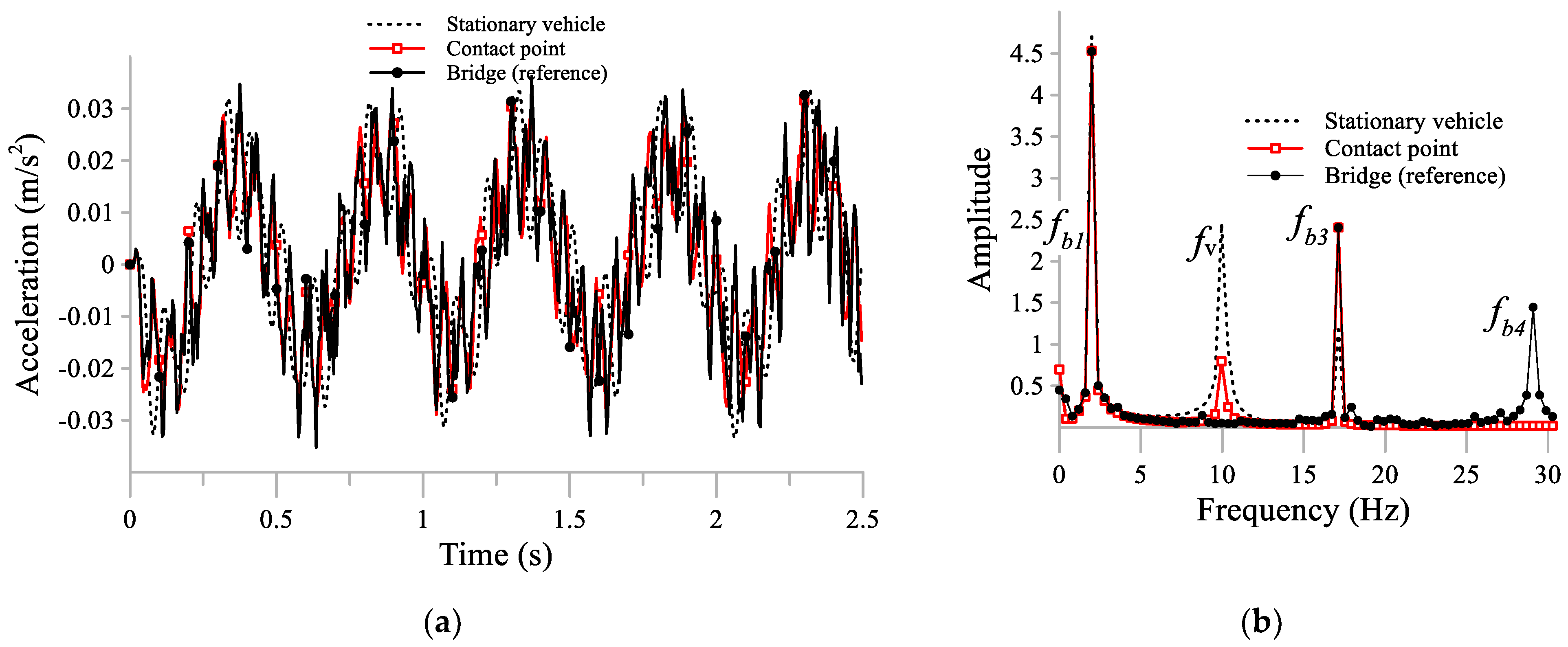
3.1.4. Vehicle Frequency Higher Than Bridge’s Second Frequency

The last case in this section shows the contact-point response of a vehicle with a frequency higher than the second frequency of the bridge (8.3 Hz). It is expected that increasing the stiffness of the stationary vehicle would increase the reliability of the recorded dynamic response. If the stiffness is increased to infinity, the vehicle would be directly mounted on the bridge, which would reflect the exact true response of the bridge; however, the scanning vehicle that is used in practice has a limited frequency. In this case, the frequency of the stationary vehicle was increased to be 10 Hz, where the stiffness of the vehicle was 800,000 N/m and the mass remained at 200 kg. Figure 8a shows the acceleration response of the stationary vehicle and its contact-point response. Unlike the previous cases, the stationary vehicle response is in good agreement with the true bridge response due to the high stiffness of the stationary vehicle. Despite that, the contact-point response still improved the response of the stationary vehicle to be more accurate, as shown in Figure 8b. The frequency of the vehicle at 10 Hz is reduced by employing the contact-point response. Also, the third mode of vibration shows an exact agreement between the true bridge response and the contact-point response.

3.2. Stationary Vehicle Damping Effects

This section investigates the effect when damping is added to the stationary vehicle. In this section and all further sections, the stationary vehicle in Section 3.1.3 with a frequency of 3.18 Hz was used. Yang and Zhang [34] used a damping ratio of 20% for a moving vehicle to compute the contact-point response. According to Calvo et al. [41], a damping ratio for a typical car ranges from 0.2 to 0.4. In this paper, a damping ratio of 0.25 was considered for the stationary vehicle. 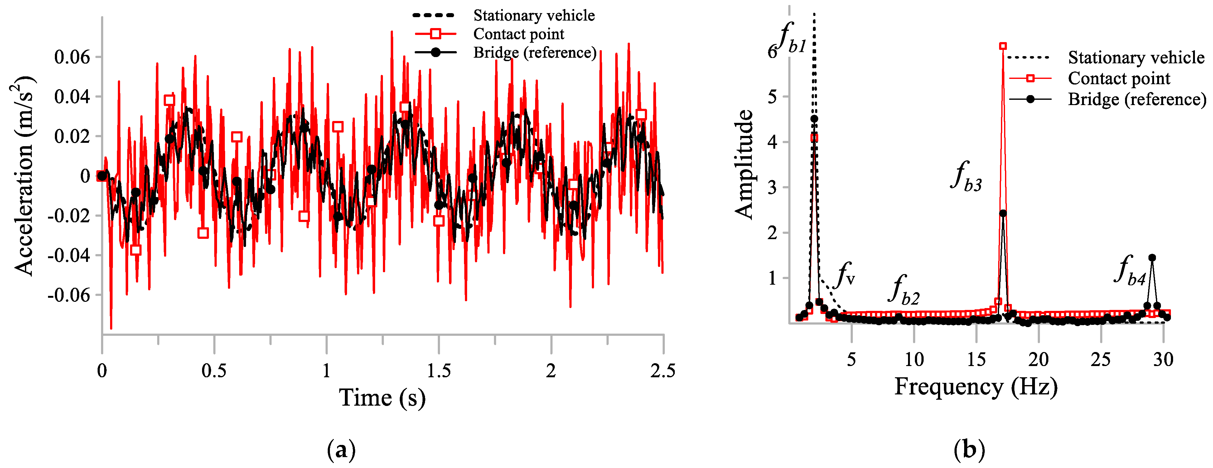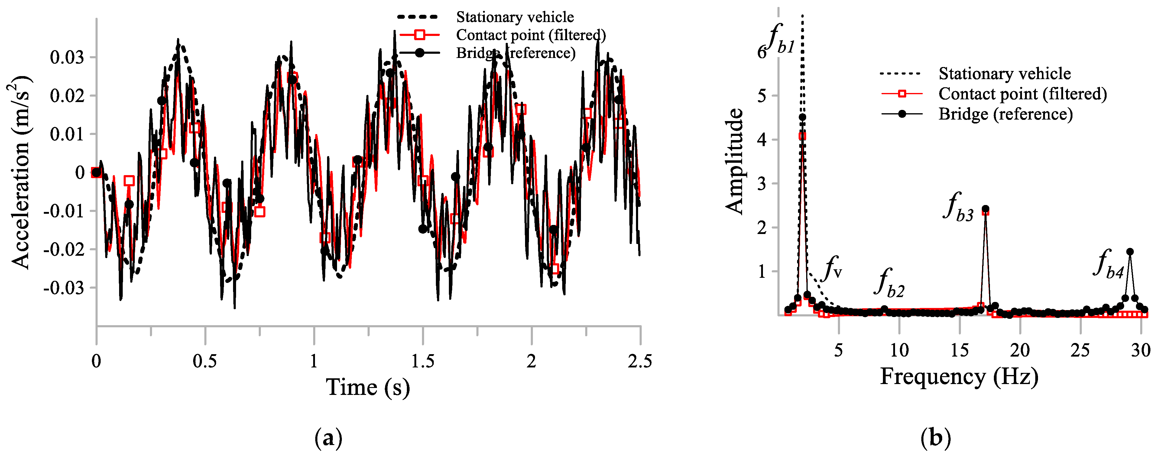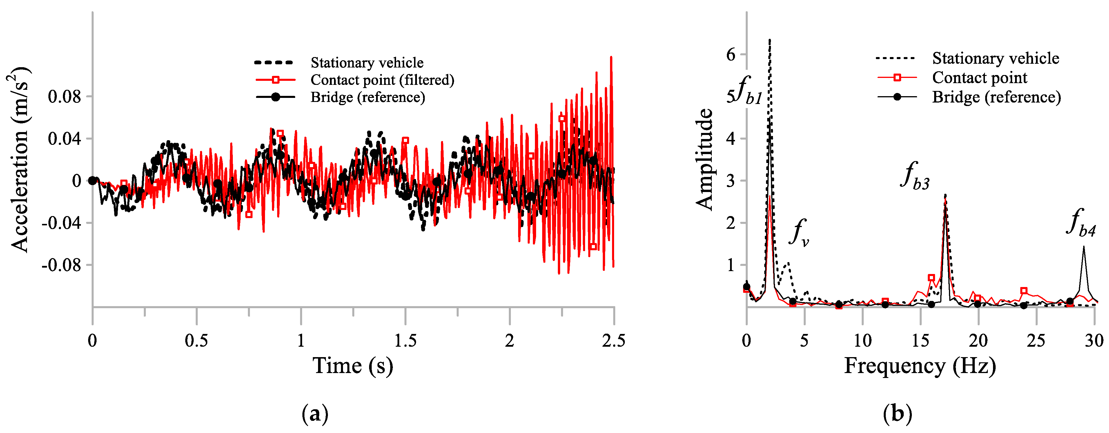Figure 9a shows the acceleration response of the damped stationary vehicle and its contact-point response. There was a noticeable difference between the contact-point response and the bridge response in the time domain. This was due to the differences between the high frequencies added to the contact-point response; however, when the frequency spectra were compared, the first mode of frequency of the contact-point agreed well with the bridge response; however, the difference in the third mode is clear between the contact-point and bridge responses. As such, a moving average filter (MAF) technique was used to filter the contact-point response as shown in Figure 10. When the filter was applied to the contact-point response, the third mode of vibration agreed well with the bridge response as shown in Figure 10b.

3.3. Stationary Vehicle Location

This section investigates the effects of the location of the stationary vehicle and its contact-point response. In the case where the stationary vehicle at 3.18 Hz was located at the mid-span location, its response and contact-point response were presented previously in Figure 5. The first and third modes of frequency of the bridge are visible in the FFT spectra of the stationary vehicle and contact-point responses as shown in Figure 5b. The second mode of frequency of the bridge is not visible in the bridge response spectrum.

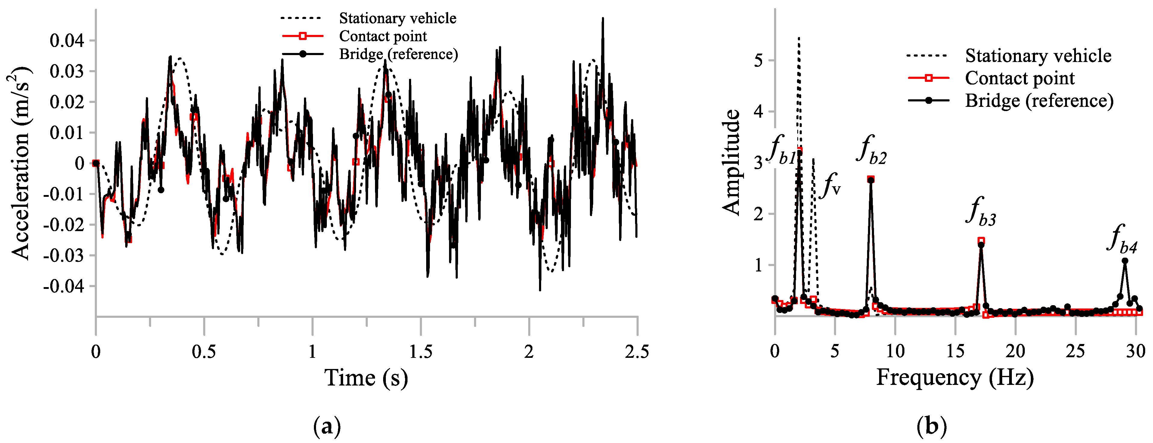
It is known that the maximum value of the second mode shape of a simply supported beam occurs at the first and third quarters of the beam. Consequently, in this section, the stationary vehicle was located at the first quarter of the beam. The stationary vehicle and its contact-point and bridge responses at the first quarter are shown in Figure 11a. Good agreement between the contact-point response and true bridge response can be observed. The acceleration spectra are shown in Figure 11b. The frequency of the vehicle is eliminated in the contact-point response. The first and second modes of frequency were captured by the stationary vehicle and its contact-point response; however, for the first and second modes, there is clear discrepancy of the stationary vehicle spectrum comparing with the true bridge spectrum, while the third mode is not even captured by the stationary vehicle response. On the other hand, the contact-point response coincides almost exactly for the first, second, and third modes of frequency.

3.4. Effect of Road Roughness

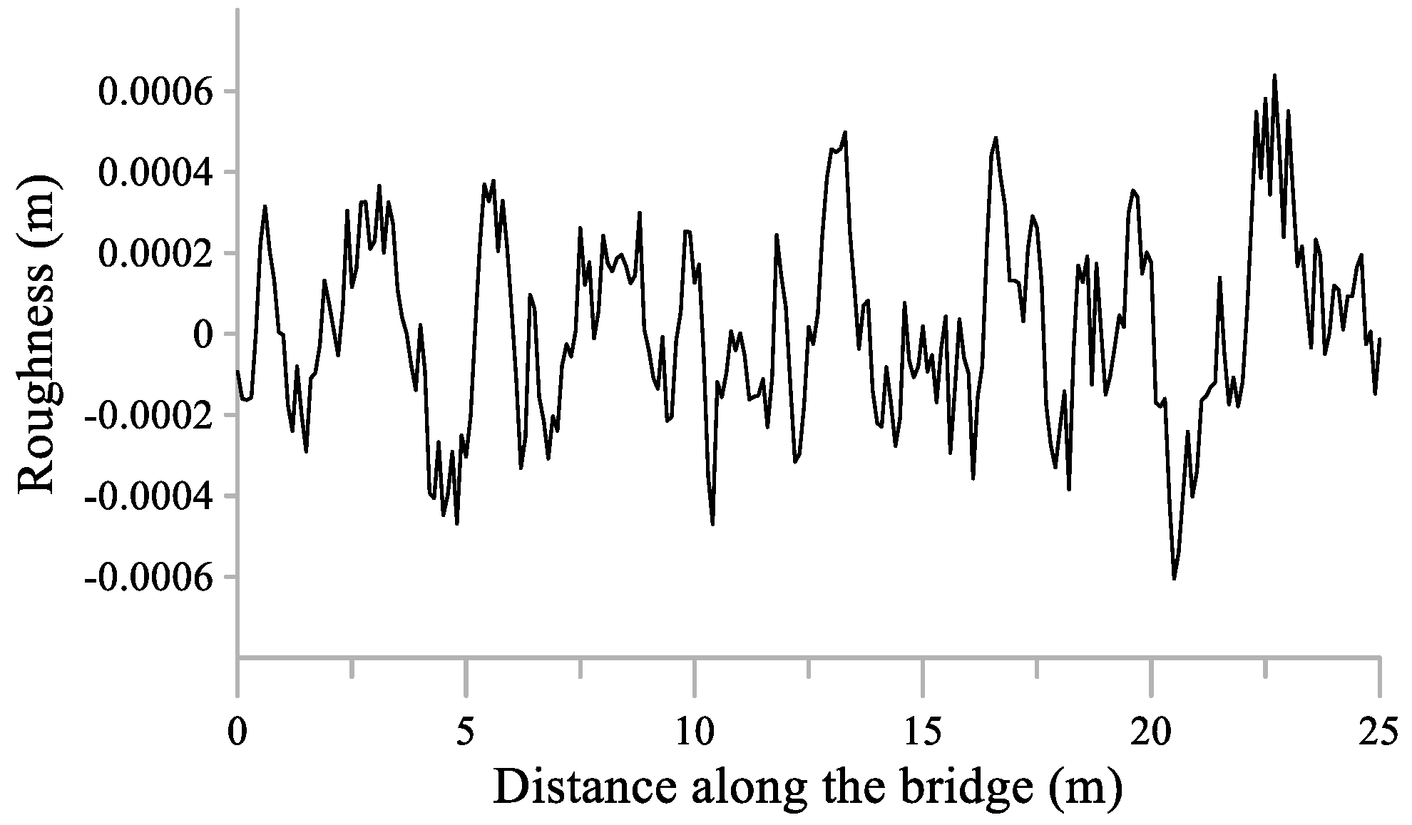
It is known that road roughness presents one of the most challenging obstacles for the use of the indirect method. As such, in this study, road roughness was added to the bridge surface simulation to investigate the response of the stationary vehicle and its contact-point response. To simulate road surface roughness, the power spectral density (PSD) functions introduced by ISO 8608 (2016) [42] were adopted in this study. Road surface roughness can be obtained as follows:

$$r(x)={\displaystyle \sum _i{d}_i}\cos ({\mathrm{n}}_i\mathrm{x}+{\theta }_i)$$

(13)

where ${\mathrm{n}}_i$ is the $ith$ spatial frequency per meter, $\mathrm{x}$ is the position on the road, ${\theta }_i$ denotes the random phase angle, and $d_i$ is the amplitude which depends on the selected roughness class. The roughness class can be determined as follows:

$$d=\sqrt{2G_d(\mathrm{n})\Delta n}$$

(14)

where the PSD function $G_d(n)$ is defined as:

$$G_d(n)=G_d(n_0){\left(\frac{n}{n_0}\right)}^{-2}$$

(15)

where n₀ is a constant that is equal to 0.1 cycle/m. In this study, the function $G_d(n_0)$ was selected for class B road surface roughness, as per ISO 8608 (2016), which is 6 × 10⁻⁶ m³. The sampling interval $\Delta n$ for the spatial frequency was selected to be 0.04 cycle/m and the lower and upper spatial frequencies were selected as 1 and 100 cycle/m, respectively. Considering the previous values, the road roughness profile was obtained as shown in Figure 12.

The previous road roughness profile was used to study the effects of road roughness on a damped and undamped stationary vehicles. The road roughness profile was added to the bridge track in the Ls-Dyna program. The road roughness is considered as the vertical displacement from line of beam elements which can be added by the function keyword of RAIL-TRACK.

3.4.1. Undamped Stationary Vehicle

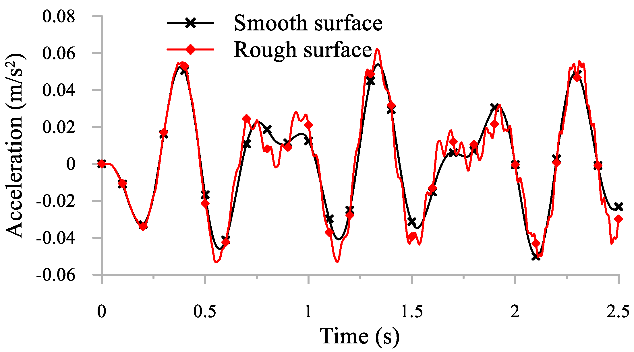
The same stationary vehicle from Section 3.1.3 at 3.18 Hz was parked on the bridge while the moving vehicle passed over a rough surface. Figure 13 shows the response of the stationary vehicle with rough and smooth surfaces. It is shown how the rough surface affects the response of the stationary vehicle.

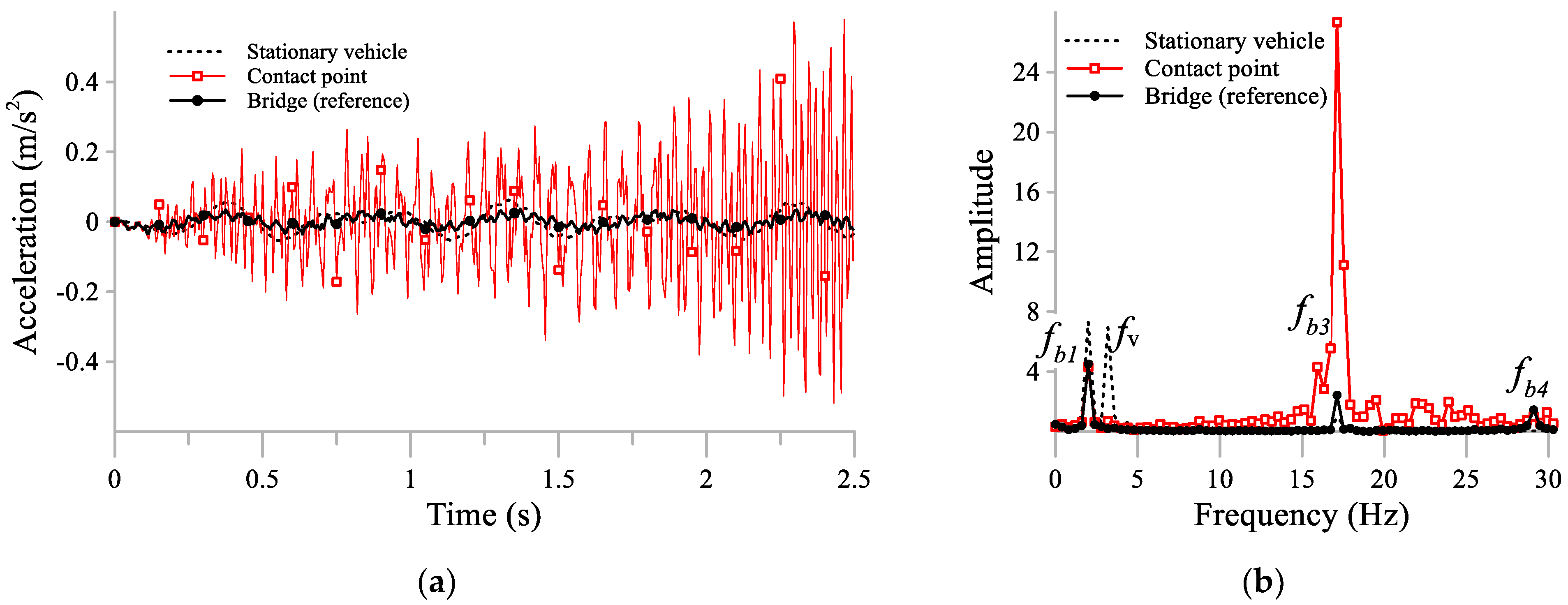
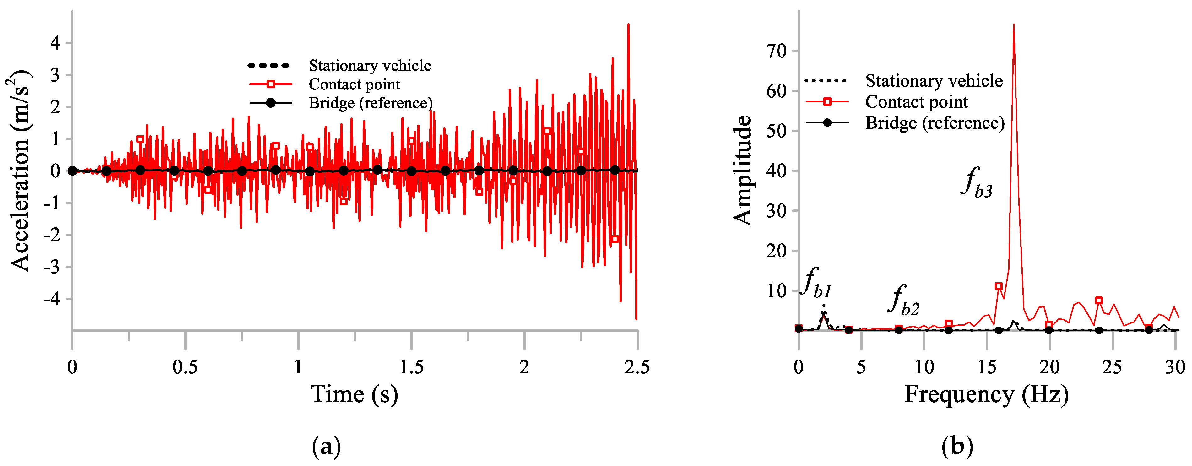
Figure 14a shows the contact-point response of the stationary vehicle on a rough surface, compared with the response of the bridge and stationary vehicle. The contact-point response is far greater than that of the true bridge response. The figure shows that higher frequencies are added to the contact-point response of the stationary vehicle. These high frequencies appear due to taking the second derivative of the irregular signal due to road roughness. Figure 14b shows the acceleration spectra of the stationary vehicle, contact-point, and bridge responses. The vehicle’s frequency at 3.18 Hz is eliminated in the contact-point spectrum; however, the contact-point response shows a high spike on the third mode and higher frequencies.

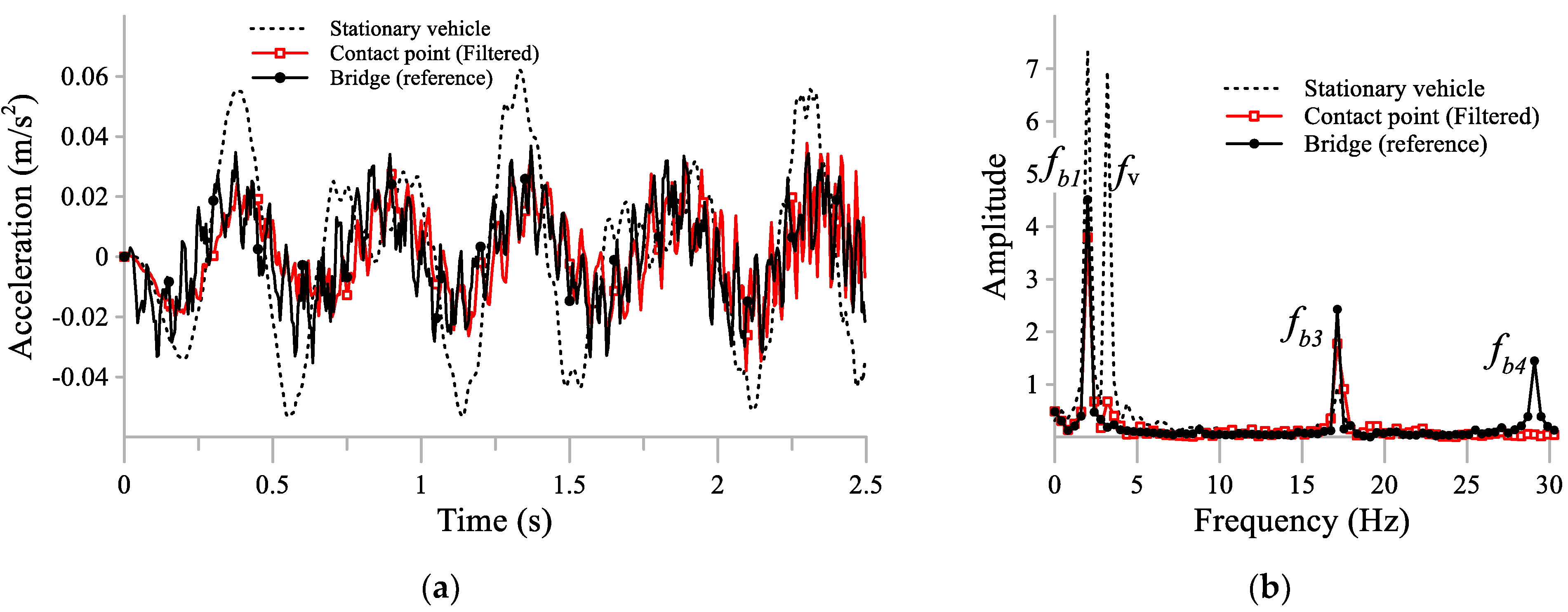
In order to remove high frequencies which corrupt signals, a moving average filtering technique has been used in another work [43]. Figure 15 shows the filtered contact point signal and its FFT spectrum. This figure shows clearly how the contact-point response has superior representation of the bridge response. The first and third modes of frequency obtained by the contact-point response agree well with the reference bridge response.

3.4.2. Damped Stationary Vehicle

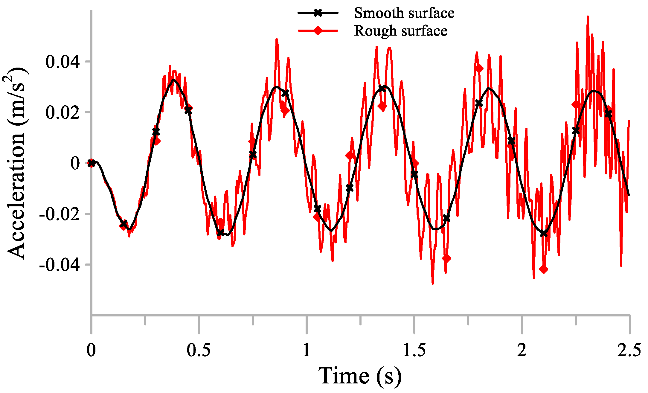
A damping ratio of 25% was added to the stationary vehicle to investigate its contact-point response for a bridge with rough surface. Figure 16 shows the response of the damped vehicle with smooth and rough surface. The response of the stationary vehicle with road roughness presents a clearly irregular form.

Figure 17 shows the contact-point response of the irregular response of the stationary vehicle (beam with rough surface). The contact-point response again shows higher frequencies, as demonstrated in Figure 17b. Again, the contact-point was filtered by the MAF technique as shown in Figure 18. The high frequency of the third mode has been eliminated as shown in in Figure 18b. Also, the vehicle’s own frequency was eliminated in the contact-point response; however, unlike other cases without damping, the stationary vehicle shows good agreement with the bridge response in the first and third modes of frequency.

3.5. Speed of the Moving Vehicle

The driving frequency is one of the components that influences the bridge response, as shown in Equations (6)–(8). This section shows the response of the stationary vehicle due to a different moving speed. The same stationary vehicle of 3.18 Hz was used from Section 3.1.3. In that section, the speed was 10 m/s. Here, the response from a different speed of 5 m/s is demonstrated. Figure 19a shows the response of the stationary vehicle and contact point due to the excitation of a vehicle moving at speed of 5 m/s. The acceleration response spectra are shown in Figure 19b. By comparing the results from the 10 m/s and 5 m/s speeds, the contact-point and the bridge responses are in good agreement, regardless of the moving vehicle speed. It can be noted that the magnitude of the response at lower speeds is small. Also, the fourth mode of vibration is not clear in the bridge response when using a speed of 5 m/s.

3.6. Mass of the Moving Vehicle

The analytical formulation presented previously shows that the moving vehicle mass may influence the dynamic response of the bridge. As such, in this section, another mass for the moving vehicle is studied. Previously, for all the cases, the mass of the moving vehicle was 1200 kg. Here, another vehicle with a mass of 7200 kg is studied. The speed of the moving vehicle is considered to be 10 m/s and the frequency of the stationary vehicle is 3.18 Hz. The acceleration responses due to the 7200 kg moving vehicle and their spectra are shown in Figure 20. The contact-point response shows good agreement with the true bridge response, regardless of the mass input of the moving vehicle. Also, it should be noted that the responses due to the 7200 kg mass of the moving vehicle exhibited higher amplitudes than those of the 1200 kg moving vehicle.

3.7. Stationary Vehicle Response on a Long Span

This section investigates the stationary vehicle response and the contact-point response for a bridge with a long span. Dusseau and Dubaisi [44] measured the frequencies of a large number of bridges in the United States. The longest span they recorded was 43 m with a theoretical frequency of 5.5 Hz and measured frequency of 3.4 Hz. As such, in this section, the bridge length was selected to be 40 m with a frequency of 4 Hz. The properties of the moving and stationary vehicles were selected to be the same as in Section 3.1.3. From Figure 21, the contact-point response could eliminate the vehicle’s frequency from the vehicle’s response. The third mode of the bridge frequency was also detected by the contact-point response. In this case, the stationary vehicle frequency is less than the fundamental frequency of the bridge; however, the response spectrum shows the fundamental frequency of the bridge clearly.

4. Conclusions

This paper has studied the contact-point response of a stationary vehicle placed on a bridge traversed by a moving load. The stationary vehicle response does not reflect the true vibration of the bridge because it contains its own frequency. Consequently, the contact-point response was calculated to eliminate this frequency. The paper investigated the factors that influence the response of the stationary vehicle, such as the stationary vehicle frequency and damping, location of the stationary vehicle, the effects of road roughness, moving vehicle speed and mass, and a longer bridge span. The acceleration responses were compared between the stationary vehicle, contact-point, and true bridge responses. Comparisons were performed in the time and frequency domains. The contact-point response showed good agreement with the true bridge response regardless of the stationary vehicle’s frequency, the mass and speed of the moving vehicle, and the bridge length. The frequency domain comparison showed that the stationary vehicle frequency was eliminated in the contact-point response. Moreover, higher frequency modes, such as the third mode of bridge vibration, could be detected using the contact-point response. In extreme cases, such as resonance, the contact-point acceleration signal still shows good agreement with that of the bridge. Higher moving vehicle speeds and masses amplify the bridge’s dynamic response; however, the agreement between the contact-point response and the true response of the bridge remains good, regardless of mass or speed.

The location of the stationary vehicle is important in determining the frequency of the bridge. The contact-point response was able to detect the true response of the bridge regardless of the location. Adding damping reduced the difference between the bridge and stationary vehicle responses, but the contact-point response still provides superior results over the stationary vehicle’s response.

Finally, road roughness is known to be an obstacle in identifying the true bridge response when considering the contact-point response of a stationary vehicle. For the cases of damped and undamped stationary vehicles, the contact-point response had a greatly amplified response with huge discrepancies regarding the response of the bridge. This is because the contact-point response depends on the second derivative of the fluctuating stationary response signal when road surface is considered. Although the stationary vehicle’s own frequency was reduced significantly, high noise frequencies due to road roughness appeared in the contact-point spectrum; however, when the contact-point response was filtered by the MAF technique, the results agreed well with those of the bridge. Nevertheless, road roughness still requires further investigation, such as considering different roughness profiles and testing other filtering techniques.