Article

Zernike Coefficient Prediction Technique for Interference Based on Generation Adversarial Network

1
Department of Electronic and Computer Engineering, National Taiwan University of Science and Technology, Taipei City 106335, Taiwan
2
Graduate Institute of Color & Illumination Technology, National Taiwan University of Science and Technology, Taipei City 106335, Taiwan
3
Graduate Institute of Applied Science and Technology, National Taiwan University of Science and Technology, Taipei City 106335, Taiwan
4
Graduate Institute of Electro-Optical Engineering, National Taiwan University of Science and Technology, Taipei City 106335, Taiwan
5
National Applied Research Laboratories, Taiwan Instrument Research Institute, Hsinchu City 30076, Taiwan
*
Author to whom correspondence should be addressed.
Appl. Sci. 2021, 11(15), 6933; https://doi.org/10.3390/app11156933
Submission received: 15 July 2021 / Revised: 23 July 2021 / Accepted: 26 July 2021 / Published: 28 July 2021
(This article belongs to the Topic Machine and Deep Learning)

Abstract

:
In the paper, we propose a novel prediction technique to predict Zernike coefficients from interference fringes based on Generative Adversarial Network (GAN). In general, the task of GAN is image-to-image translation, but we design GAN for image-to-number translation. In the GAN model, the Generator’s input is the interference fringe image, and its output is a mosaic image. Moreover, each piece of the mosaic image links to the number of Zernike coefficients. Root Mean Square Error (RMSE) is our criterion for quantifying the ground truth and prediction coefficients. After training the GAN model, we use two different methods: the formula (ideal images) and optics simulation (simulated images) to estimate the GAN model. As a result, the RMSE is about 0.0182 ± 0.0035λ with the ideal image case and the RMSE is about 0.101 ± 0.0263λ with the simulated image case. Since the outcome in the simulated image case is poor, we use the transfer learning method to improve the RMSE to about 0.0586 ± 0.0035λ. The prediction technique applies not only to the ideal case but also to the actual interferometer. In addition, the novel prediction technique makes predicting Zernike coefficients more accurate than our previous research.

1. Introduction

Aberration is the difference between an actual image and an ideal image in the optical system. Therefore, aberration is one of the essential reference indicators when designing an optical system. Usually, the aberration of a system is quantified when evaluating the system’s performance, such as Seidel aberrations [1] and Zernike polynomials [2]. For example, the Zernike polynomials use a series of orthogonal polynomials for the unit circle [3].
One method to measure aberration is an interferometer. The aberration information is recorded on the interference fringe image. Therefore, Zernike coefficients could be calculated using traditional optical equations, such as the interference phase shift method, the Fourier transform method, and the phase-shift method. The conventional conversion methods convert interference fringe images to Zernike coefficients and require two steps, which are complex mathematical calculations. First, the interference fringe image is converted into the wavefront difference or phase difference. Second, Zernike coefficients are calculated using the surface fitting method with Zernike polynomials [4].
To simplify the calculation process, we use deep learning to obtain the Zernike coefficients from interference fringe images. A neural network learns from a lot of training datasets. After finishing the training, the model predicts the answer for the new image [5]. Therefore, this method does not need complex mathematical calculations and can expect the answers needed. In this paper, we use the Generative Adversarial Network (GAN) to predict Zernike coefficients quickly and simply.
Goodfellow and others proposed the GAN model in 2014 to achieve unsupervised learning of adversarial networks [6]. The network architecture of the GAN model is composed of two networks as follows: the Generator network and the Discriminator network [7]. The goal of the Generator network is to generate images that are close to authentic images. The Discriminator network is an auxiliary role for training the Generator network to achieve unsupervised learning. The concept of Pix2Pix is an image-to-image conversion method uses applications of the GAN model. Therefore, the GAN model generates training datasets, image recognition, image inpainting, and fake photography using human image synthesis technology (DeepFake) [8,9,10,11,12,13,14,15,16,17,18,19]. In previous research, many studies focused on fringe and aberration using deep learning [20,21,22,23,24], and we used GoogLeNet to predict Zernike coefficients [25]. The prediction accuracy is good but not good enough, so we study GAN to improve the prediction accuracy.
According to the advantage of GAN image-to-image translation, we propose a novel usage for GAN in this paper. We design a mosaic image as the output image of the Generator, and each piece of the mosaic image links to the number of Zernike coefficients. That is a new concept of GAN for image-to-number translation. Therefore, we use GAN to predict Zernike coefficients (mosaic image) from interference fringe images directly. First, the training datasets are generated by Python with an optics formula since the interferometer cannot easily create many interference fringe images as the Generator’s inputs. Then, we use optical software, VirtualLab (VL), to generate simulated images and to transfer learning to improve the accuracy with almost actual interference fringe images [26,27]. According to the result, the prediction technique can predict the Zernike coefficients of an interference fringe from the interferometer in the future.

2. Methods

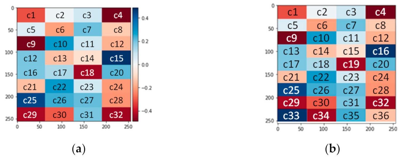
2.1. Datasets for GAN Model

We need two input images, for the Generator and the Discriminator networks, to train the GAN model. First, we generate images as the input of the Generator network based on the optics formula in Python since the interferometer cannot easily obtain many actual pictures in a short time. We need to sequentially generate the phase difference and the interference fringe based on two formulas. The phase difference formula is represented by Zernike polynomials based on a polar coordinate system, as shown in Equation (1).
δ r , θ = n = 1 N a n z n r , θ
where the δ represents the appearance of the phase difference, an represents the value of the nth Zernike coefficients, and zn represents the nth item in the polynomials. In this paper, the range of an is −0.5–0.5, radius r is 0–1, angle θ is 0–2π, and order n is 1–32. When producing the datasets, the Zernike coefficients are set randomly. The piston term in the first order of the Zernike mode should be ignored because it does not affect the wavefront distribution. Additionally, we do not analyze the piston term. Moreover, each Zernike polynomials item represents a kind of aberration meaning and the coefficient is a quantitative aberration.
Then, we use the phase difference to calculate the interference fringe based on the interference fringe formula, as shown in Equation (2), where Ia is the reference light and Ib is the tested light. Since the interference fringe formula is a series of the cosine function, the positive and negative values of Zernike coefficients may have a chance to produce the same interference fringes. Therefore, these datasets should not be used for model training because one input fringe image corresponds to more than one series of coefficients. To solve this problem, we use the phase shift method to make the GAN model distinguish between positive and negative values of Zernike coefficients.
I = I a + I b + 2 I a I b cos δ
According to the phase-shift method, we use two interference fringes, including the original interference fringe and the reference fringe based on the phase difference adding π/4, as shown in Equations (3) and (4). Regarding how to combine the two images for the model’s input, a previous paper divided the two interference fringes for generating one input image [25]. However, during the training process, there is a phenomenon of divergence or overfitting when we only divided the two fringes. Therefore, this paper further uses the logarithmic divided fringes in our training experience, as shown in Equation (5). The possible reason is that some of the I’ values are too large when the I2 values are too small or close to zero. Therefore, the input interference fringe images are adjusted in this paper, and the training dataset is different from the previous article [25]. The image size is 256 × 256 pixels.
I 1 = I a + I b + 2 I a I b cos δ
I 2 = I a + I b + 2 I a I b cos δ + π 4
I = log I 1 I 2
Second, we also generate the ground truth, with Zernike coefficients as one of the Discriminator’s inputs; another input is a fake image that is the output of the Generator network. The actual image is designed with 32 equal pieces, and each part corresponds to one of the Zernike coefficients. The image size is 256 × 256 pixels, so each piece has 2048 pixels. An example of the target image looks similar to a mosaic image, and the size of each piece is 32 × 64 pixels, as shown in Figure 1a, where c1 is the first Zernike coefficient and c2 is the second Zernike coefficient, etc. Therefore, the GAN becomes the image-to-number translation network.
The Generator’s output is also the mosaic image that corresponded to the Zernike coefficients. In the output image, the pixel value of each piece is the predicted coefficient. Therefore, the 32 predicted values are the average of 30 × 62 pixels but without the edge of the region. Since the edge pixels have a more significant chance of producing uncertain values and of influencing the accuracy, we removed the edge pixels of each piece for checking the Generator’s output.
Furthermore, the predicted number of Zernike coefficients can be increased, and the target image are also divided into more elements. An example of the designed image for 36 Zernike coefficients is shown in Figure 1b. c1 is the first Zernike coefficient, and c2 is the second Zernike coefficient, etc.

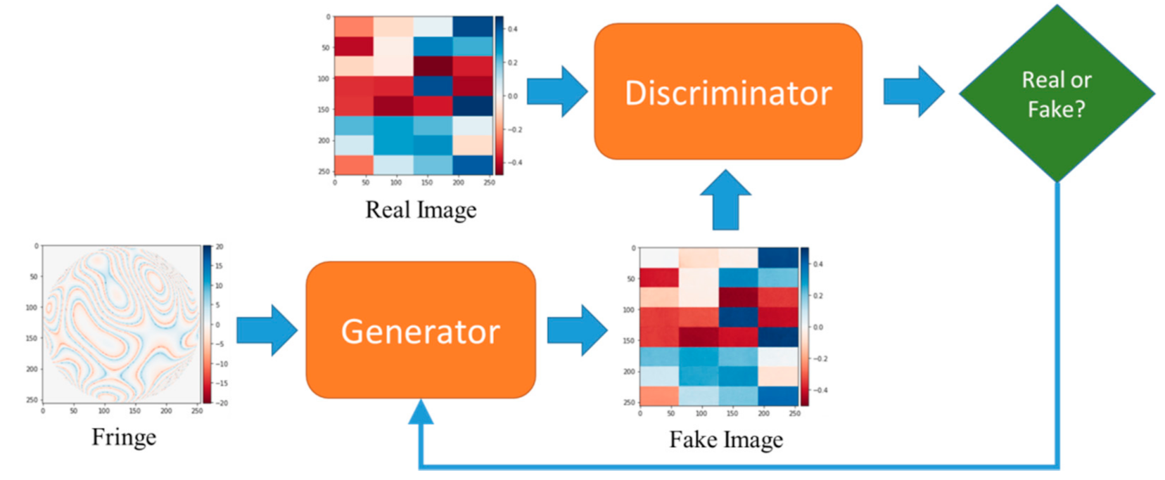
2.2. Generative Adversarial Network (GAN)

In the paper, we use Generative Adversarial Network (GAN) to predict 32 Zernike coefficients. A Generator network and a Discriminator network consist of a GAN model. The following introduces the architecture of networks, training model, and the architecture of experimental.

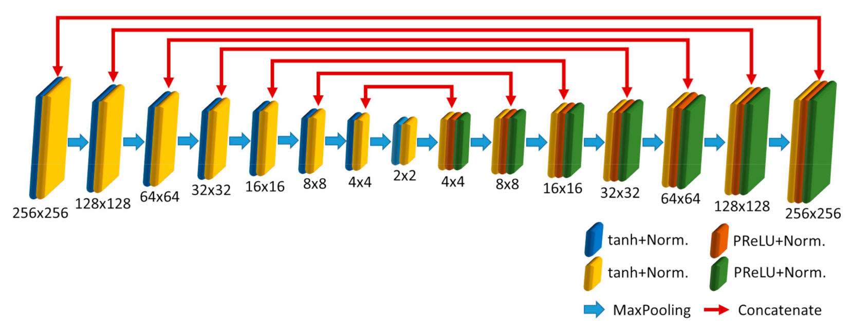
2.2.1. The Generator Network

The Generator network is a Convolutional Neural Network (CNN) with the U-Net structure. As shown in Figure 2, the Generator consists of seven down-sampling layers of CNN and seven up-sampling layers of CNN. The Generator’s input is the logarithmic divided fringes, and the output is the fake image for predicting the Zernike coefficients. As the down-sampling layers are used to extract the features from the input, the data are reconstructed by up-sampling layers to increase the data size for output. In the down-sampling layers, one layer comprises two 2 × 2 convolutional layers, two normalization layers, and one 2 × 2 max-pooling layer. In the up-sampling layers, one layer consists of one 2 × 2 convolution transpose layer, two 2 × 2 convolutional layers, two normalization layers, and one 2 × 2 max-pooling layer in which the convolution transpose layer concatenates with the corresponded layer of the down-sampling structure. Moreover, the down-sampling network uses the hyperbolic tangent (tanh) activation function, and the up-sampling form uses the parametric rectified linear unit (PReLU) activation function. The normalization layers of the Generator network are Instance Normalization.

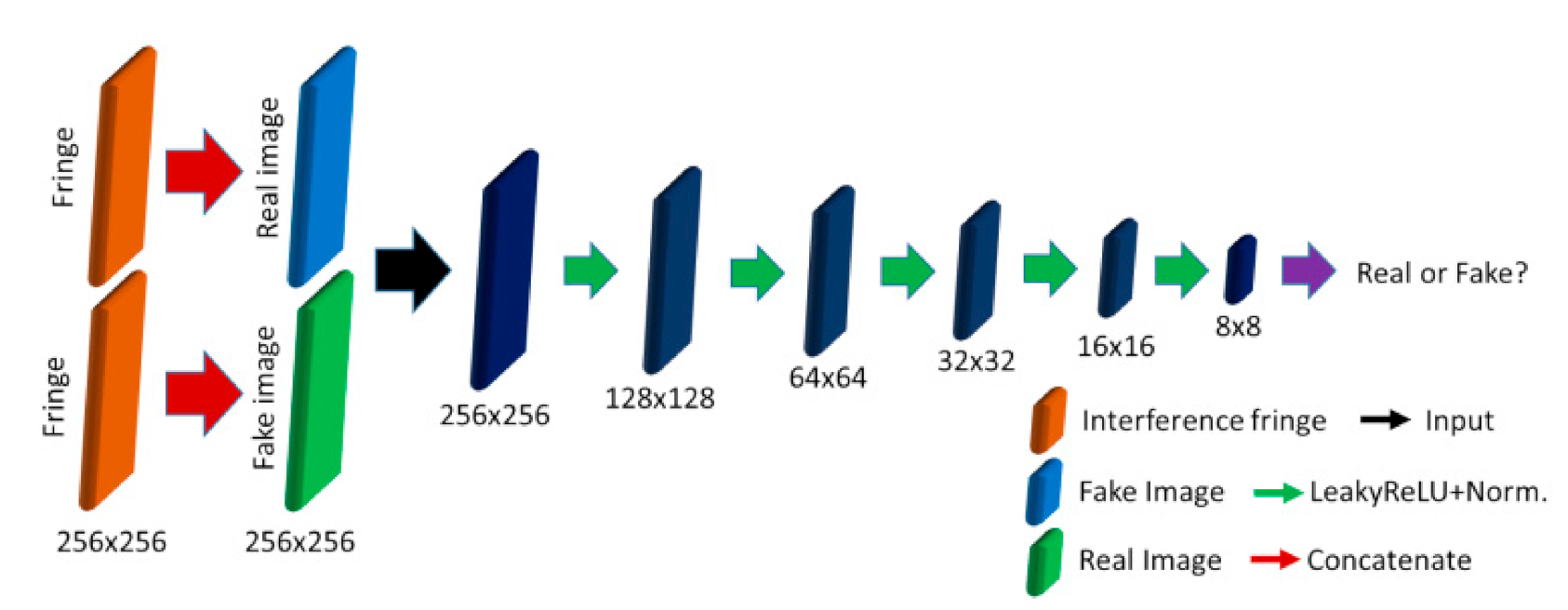
2.2.2. The Discriminator Network

The Discriminator network represents a convolutional PatchGAN classifier and learns to classify the Generator’s output image as real or fake, as shown in Figure 3. Since the Discriminator network has a classifier function for the Generator network, GAN becomes an unsupervised learning network. The PatchGAN has three purposes: to reduce the number of parameters, to avoid overfitting, and to decrease the training time of the model. The Discriminator network includes four down-sampling layers, and one layer composes one 4 × 4 convolution layer and one normalization layer. The activation function uses a leaky rectified linear unit (LeakyReLU), and the normalization layers are Bench Normalization except the second, that is Instance Normalization. Finally, the Discriminator’s output is 8 × 8 pixels to judge the real and fake images.

2.2.3. Training GAN Model

We use the Colab service provided by Google for training the GAN model. First, the parameters of the Discriminator network are updated with the initial fake image and actual image, but the Generator network is maintained. Second, the parameters of the Generator network are updated with the interference fringe image and the Discriminator’s output that is the judgment of the fake photo, but the Discriminator network is maintained. Third, the Discriminator network is renewed again with the Generator’s output image, a fake image, and the ground truth image, but the Generator network is maintained. Fourth, the Generator network is renewed with the interference fringe image and the judgment of fake picture, but the Discriminator network is maintained. Then, these two networks are trained interactively, as shown in Figure 4.
The actual image is the ground truth image generated by the formulas with Zernike coefficients. The fake image is the Generator’s output image, and it gradually approximates the actual picture during the training process. The Discriminator’s output is the judgment of a fake photo and can help the Generator update parameters. The training process of the GAN model is to maximize the discriminator loss function and to minimize the generator loss function.
The randomly generated datasets include 400 training images and 40 validation images. The total training epochs are 700 epochs for converging during the five iterations of the training processes. The Generator’s optimizer is Root Mean Square Prop (RMSProp), and the learning rate is fixed at 0.001. The Discriminator’s optimizer is the Stochastic gradient descent (SGD), and the initial learning rate is 0.00002, used on the first two processes and then become one-tenth for each following procedure. Finally, we obtain the pre-trained model when the training process is complete.

2.2.4. Testing GAN Model

We also use the Colab service provided by Google to test the GAN model (pre-trained model). The test process includes two different fringe datasets in the paper, based on the formula as an ideal image and optics software as an approximate actual image, to estimate the GAN model. The fringe datasets input the Generator network to test the model, and the Generator predicts fake pictures. The testing datasets in the ideal images are different from the training datasets. According to the image-to-number translation, 32 Zernike coefficients are calculated from a fake photo and then use the quantified ground truth (target image) and the Generator’s output (fake image) to calculate the RMSE. When the RMSE is smaller, the fake photo is closer to the target image. The process of testing and transfer learning is shown in Figure 5.
Testing_1 with an ideal image: The testing datasets are generated randomly by Python with the optics formula for testing the Generator. The testing datasets have 1000 photos and are inputted into the Generator. Additionally, then, the Generator’s outputs, fake images, are translated to Zernike coefficients to obtain an averaged RMSE from 1000 tests.
Testing_2 with a simulated image: The testing datasets are generated randomly by VL with a Fizeau interferometer for testing the Generator. The testing datasets have ten simulated images and are inputted into the Generator. Additionally, then, the Generator’s outputs, fake photos, are translated to Zernike coefficients to obtain an averaged RMSE from ten tests.
Transfer learning with the simulated image: The training datasets are generated randomly by VL with a Fizeau interferometer for retraining the pre-trained model. The training datasets have 100 simulated images and are inputted into the pre-trained model to acquire a new GAN model. The training datasets (100 simulated images) do not include the testing datasets (ten simulated images). After finishing the transfer learning, we use the Testing_2 process to test the new Generator with the same testing datasets to gain the new testing result to increase accuracy.

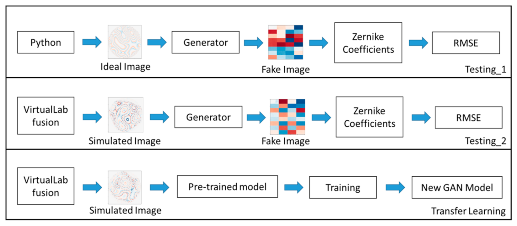
2.3. The Architecture of Experimental
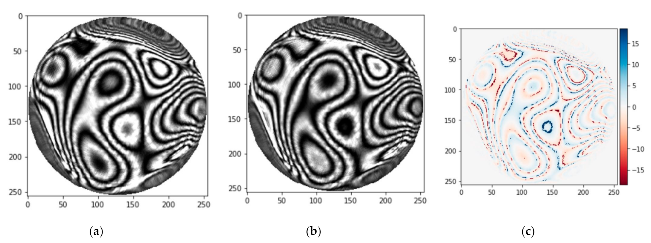
In the paper, we use the same way to estimate the GAN model from the previous article [25]. VirtualLab fusion (VL) is a simulation software based on the field tracing concept, and it can calculate approximate authentic interference fringe images. To obtain the fringe images, we build a Fizeau interferometer in VL to simulate various interference fringe with different aberration coefficients. That helps us evaluate the performance of the GAN model more authentically.

3. Results

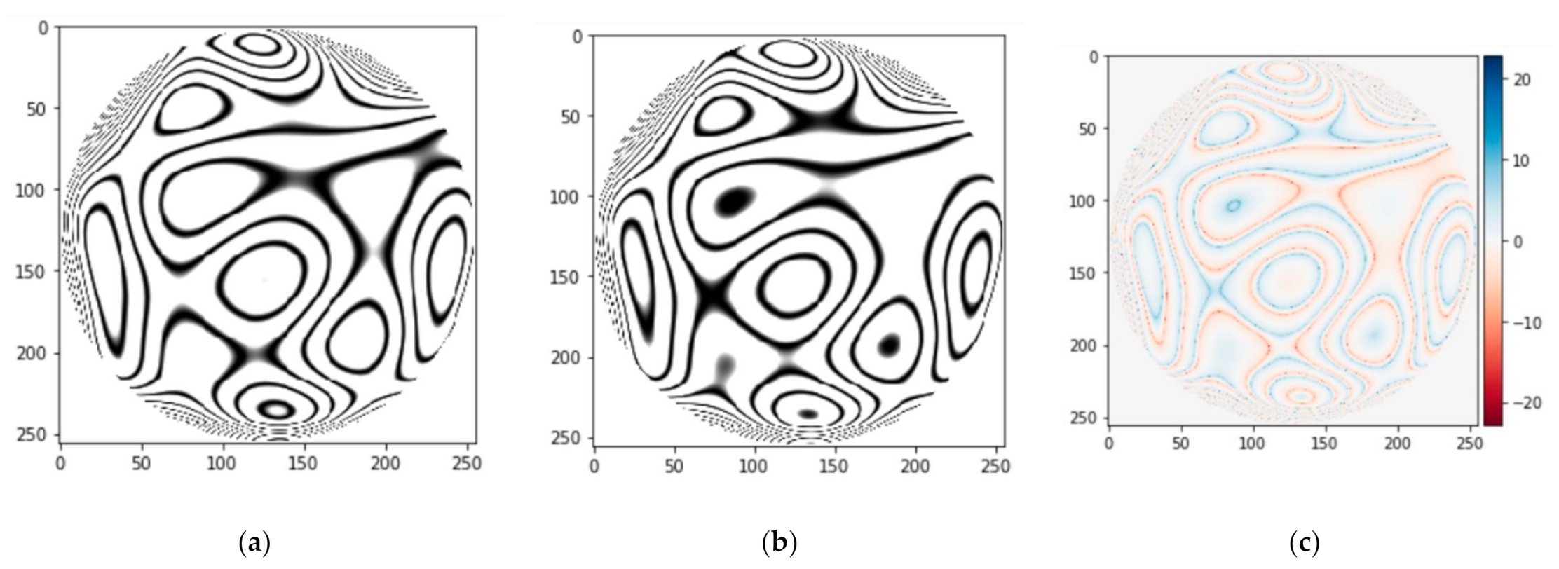
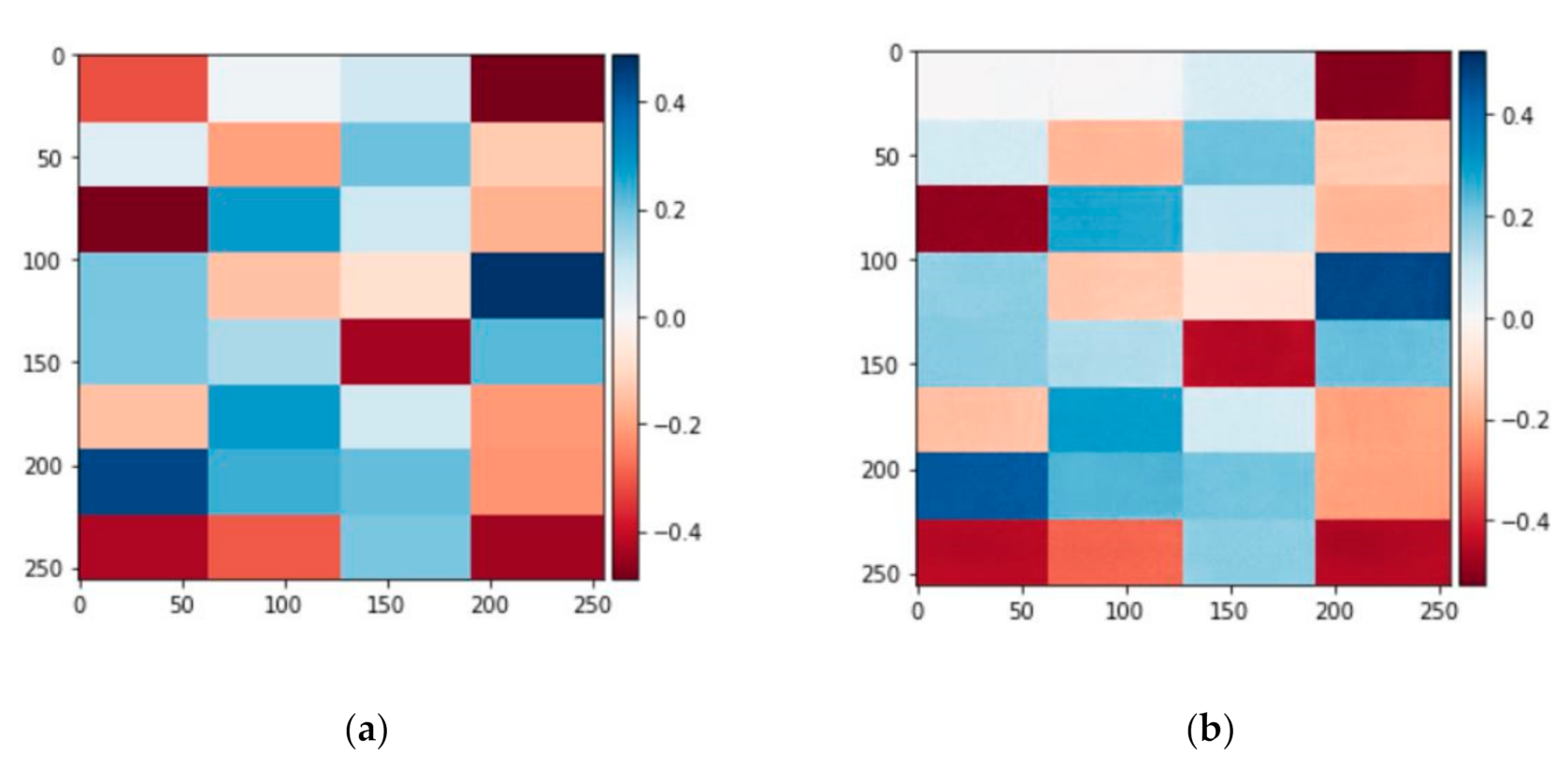
3.1. Testing_1 with Ideal Images

The testing process must be executed since we should understand the model’s performance after the training process. According to the Testing_1 process, the Generator predicts 1000 fake images using the ideal image of interference fringe and obtains 1000 RMSE. After averaging the 1000 RMSE values, the result is about 0.0182 ± 0.0035λ. For example, one testing image of the interference fringe as the input of the pre-trained model is shown in Figure 6, and the target image is shown in Figure 7a. Then, the Generator outputs the fake photo, as shown in Figure 7b. The comparison between the Zernike coefficients and predicted values is shown in Figure 8, and we do not show the difference of the first coefficient because the effect is negligible.

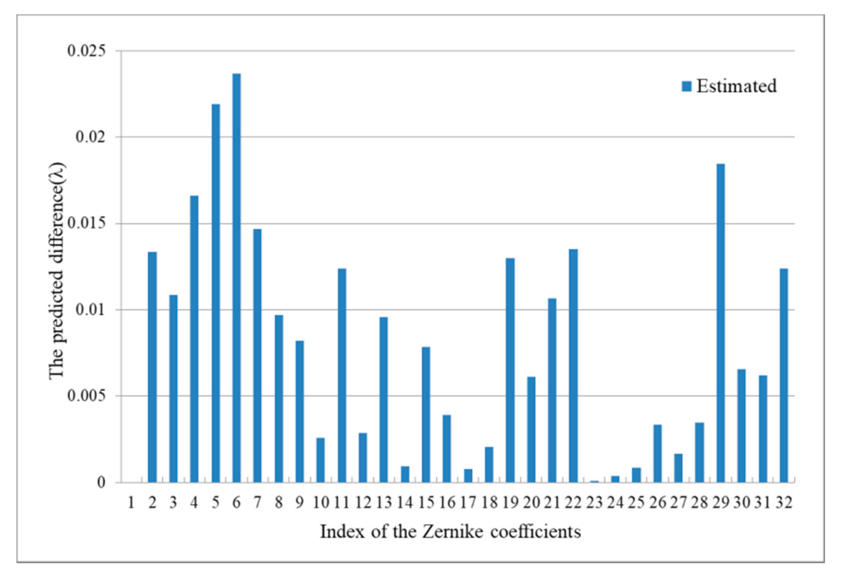
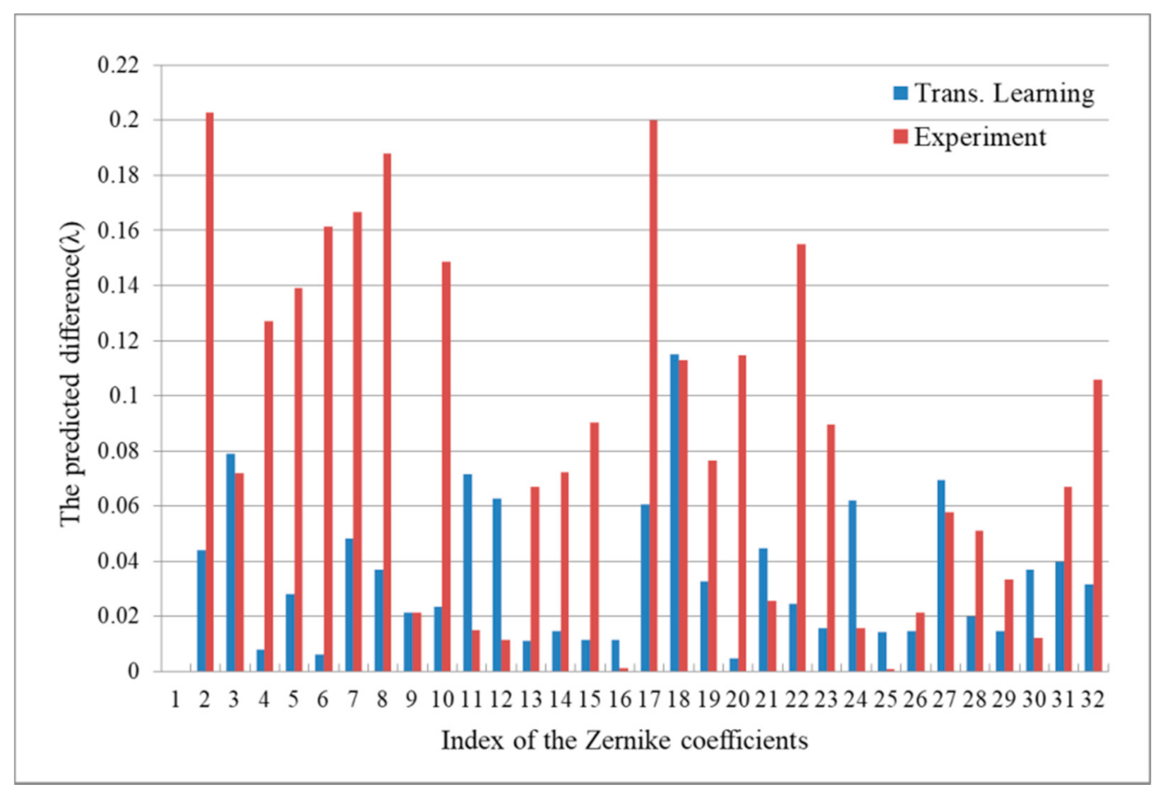
3.2. Testing_2 and Transfer Learning with Simulated Images

To understand the applicability of the GAN model and whether it can predict the coefficient with the actual interference fringes, the simulated images are used to test the GAN model. According to the Testing_2 process, the Generator makes ten fake images using the simulated image of interference fringe and obtains ten RMSE. After averaging the ten RMSE values, the result is about 0.101 ± 0.0263λ in which some of the predicted values of Zernike coefficients have significant errors. The prediction accuracy with the simulated image is worse than the ideal image since the image has more image details, and the training datasets do not include this kind of data.
For these reasons, the GAN model needs to be trained again using the transfer learning process with 100 simulation images. After the transfer learning process, the new GAN model is acquired, and it is tested again using ten of the same simulated images. After averaging the ten RMSE values, the result is about 0.0586 ± 0.0183λ. The new GAN model is better than the pre-trained model, and the tested RMSE is reduced to 0.0424λ. Therefore, we prove that the transfer learning can improve the prediction accuracy of the GAN model
For example, one simulated image of the interference fringe as the input of the GAN model is shown in Figure 9, and it is closer to the actual image than the ideal image. The comparison between the Zernike coefficients and predicted values is shown in Figure 10, and we do not show the difference of the first coefficient because the effect is negligible.

3.3. Summary

We proposed a prediction technique to predict Zernike coefficients based on GoogLeNet with an interference fringe in a previous paper [25]. After continuous research, we found a novel usage of GAN that can effectively improve the prediction accuracy. RMSE is an evaluation criterion for comparison with the two different methods. The lower RMSE is a better prediction technique than another.
We use two different methods: the formula (ideal images) and optics simulation (simulated images) to compare the performance of two networks. In the first case, the RMSE using GoogLeNet is about 0.055 ± 0.021λ, and using GAN, it is about 0.0182 ± 0.0035λ, as shown in Table 1. In the second case, the RMSE using GoogLeNet is about 0.095 ± 0.018λ, and using GAN, it is about 0.101 ± 0.0263λ. After the transfer learning, the RMSE using GAN improved to about 0.0586 ± 0.0183λ, as shown in Table 2. Therefore, the prediction accuracy of the GAN is better than that of GoogLeNet.
The time consumption of the prediction technique is another significant issue. After predicting 1000 times, the two averaged time consumptions are 0.0101 s using GoogLeNet [25] and 0.0634 s using GAN, as shown in Table 3, where the Colab service with a GPU provided by Google was used. Although the time consumption of the GAN is longer than that of GoogLeNet, the accuracy of the GAN is relatively better. Moreover, the RMSE can be reduced by 0.0364λ.

3.4. The Advantage of the GAN Model

In this paper, the novel usage of the GAN model is different from before. The Generator’s output is a fake image that links to the prediction values. GAN changes from an image-to-image translation network to an image-to-number translation network. Based on this method, we only need to adjust the designed image (fake image and target image) if the number of Zernike coefficients is increased to 36, as shown in Figure 1b. Additionally, we then used the modified datasets to train and test the GAN model. Moreover, the RMSE is about 0.0451 ± 0.0237λ with the ideal image, and the result is also better than that in a previous article [25]. This means that the GAN model can predict more or less Zernike coefficients but does not need to change any layers or parameters.

4. Discussion and Conclusions

The paper proposes a novel prediction technique to predict Zernike coefficients based on the GAN structure with the interference fringe image. Moreover, the GAN becomes an image-to-number translation network, which is a novel usage of GAN. After the testing and transfer learning, the RMSE is about 0.0182 ± 0.0035λ with the ideal image and about 0.0586 ± 0.0183λ with the simulated image.
In the paper, we achieved four significant points: the prediction accuracy is better than that in our previous research, transfer learning is used to help the model adapt the quality of the simulated image, GAN can predict more or fewer coefficients but only needs to adjust the designed image, and GAN becomes a flexible network for predicting pictures or values.
In the future, we will improve and retrain the prediction technique with the Spatial Light Modulator (SLM) to expand the generalization for the actual fringe images from the interferometer. Additionally, the new GAN usage can increase the possibility of applications in other different research fields.

Author Contributions

Conceptualization, A.J.-W.W. and Y.-Y.C.; methodology, T.-H.Y. and C.-T.L.; software, T.-H.Y.; validation, C.-T.L.; formal analysis, Y.-Y.C.; investigation, Z.-J.J.; resources, C.-H.C.; data curation, T.-H.Y.; writing—original draft preparation, T.-H.Y.; writing—review and editing, Y.-Y.C.; visualization, C.-T.L.; supervision, A.J.-W.W.; project administration, Y.-Y.C.; funding acquisition, Y.-Y.C. All authors have read and agreed to the published version of the manuscript.

Funding

This research was funded by the Ministry of Science and Technology, Taiwan, grant number 109-2221-E-011-030-.

Conflicts of Interest

The authors declare no conflict of interest.

References

  1. Kidger, M. Importance of aberration theory in understanding lens design. In Proceedings of the Fifth International Topical Meeting on Education and Training in Optics, Delft, The Netherlands, 19–21 August 1997; Volume 3190, pp. 26–33. [Google Scholar]
  2. Lakshminarayanan, V.; Fleck, A. Zernike polynomials: A guide. J. Mod. Opt. Opt. 2011, 58, 545–561. [Google Scholar] [CrossRef]
  3. Gurov, I.; Volynsky, M. Interference fringe analysis based on recurrence computational algorithms. Opt. Lasers Eng. 2012, 50, 514–521. [Google Scholar] [CrossRef]
  4. Malacara-Hernandez, D.; Carpio-Valadez, M.; Sanchez-Mondragon, J.J. Wavefront fitting with discrete orthogonal polynomials in a unit radius circle. Opt. Eng. 1990, 29, 672–676. [Google Scholar] [CrossRef]
  5. Hinton, G.E.; Osindero, S.; Teh, Y.W. A fast learning algorithm for deep belief nets. Neural Comput. 2006, 18, 1527–1554. [Google Scholar] [CrossRef]
  6. Goodfellow, I.; Pouget-Abadie, J.; Mirza, M.; Xu, B.; Warde-Farley, D.; Ozair, S.; Courville, A.; Bengio, Y. Generative adversarial nets. Adv. Neural Inf. Process. Syst. 2014, 27, 2672–2680. [Google Scholar]
  7. Mirza, M.; Osindero, S. Conditional Generative Adversarial Nets. Deep Learning and Representation Learning Workshop. arXiv 2014, arXiv:1411.1784. [Google Scholar]
  8. Yi, Z.; Zhang, H.; Tan, P.; Gong, M. DualGAN: Unsupervised Dual Learning for Image-to-Image Translation. In Proceedings of the International Conference on Computer Vision (ICCV), Lido di Venezia, Venice, Italy, 22–29 October 2017. [Google Scholar]
  9. Liu, M.Y.; Breuel, T.; Kautz, J. Unsupervised image-to-image translation networks. arXiv 2017, arXiv:1703.00848v6. [Google Scholar]
  10. Long, J.; Shelhamer, E.; Darrell, T. Fully convolutional networks for semantic segmentation. In Proceedings of the IEEE Conference on Computer Vision and Pattern Recognition (CVPR), Boston, MA, USA, 7–12 June 2015; pp. 3431–3440. [Google Scholar]
  11. Szegedy, C.; Vanhoucke, V.; Ioffe, S.; Shlens, J.; Wojna, Z. Rethinking the inception architecture for computer vision. In Proceedings of the IEEE Conference on Computer Vision and Pattern Recognition, Las Vegas, NV, USA, 27–30 June 2016; pp. 2818–2826. [Google Scholar]
  12. Huang, Y.; Lu, Z.; Shao, Z.; Ran, M.; Zhou, J.; Fang, L.; Zhang, Y. Simultaneous denoising and super-resolution of optical coherence tomography images based on generative adversarial network. Opt. Express 2019, 27, 12289–12307. [Google Scholar] [CrossRef]
  13. Yu, Z.; Zhong, Y.; Gong, R.H.; Xie, H. Filling the binary images of draped fabric with pix2pix convolutional neural network. J. Eng. Fibers Fabr. 2020, 15, 1–6. [Google Scholar] [CrossRef]
  14. Barbastathis, G.; Ozcan, A.; Situ, G. On the use of deep learning for computational imaging. Optica 2019, 6, 8. [Google Scholar] [CrossRef]
  15. Wang, M.; Guo, W.; Yuan, X. Single-shot wavefront sensing with deep neural. Opt. Express 2021, 29, 3467–3478. [Google Scholar]
  16. Yu, F.; Wang, L.; Fang, X.; Zhang, Y. The Defense of Adversarial Example with Conditional Generative Adversarial Networks. Secur. Commun. Netw. 2020, 2020, 3932584. [Google Scholar] [CrossRef]
  17. Sargent, G.C.; Ratliff, B.M.; Asari, V.K. Conditional generative adversarial network demosaicing strategy for division of focal plane polarimeters. Opt. Express 2020, 28, 38419–38443. [Google Scholar] [CrossRef]
  18. Moon, I.; Jaferzadeh, K.; Kim, Y.; Javidi, B. Noise-free quantitative phase imaging in Gabor holography with conditional generative adversarial network. Opt. Express 2020, 28, 26284–26301. [Google Scholar] [CrossRef]
  19. Zhang, H.; Zhu, T.; Chen, X.; Zhu, L.; Jin, D.; Fei, P. Super-resolution generative adversarial network (SRGAN) enabled on-chip contact microscopy. J. Phys. D Appl. Phys. 2021, 54, 394005. [Google Scholar] [CrossRef]
  20. Saha, D.; Schmidt, U.; Zhang, Q.; Barbotin, A.; Hu, Q.; Ji, N.; Booth, M.J.; Weigert, M.; Myers, E.W. Practical sensorless aberration estimation for 3D microscopy with deep learning. Opt. Express 2020, 28, 29044–29053. [Google Scholar] [CrossRef]
  21. Kando, D.; Tomioka, S.; Miyamoto, N.; Ueda, R. Phase Extraction from Single Interferogram Including Closed-Fringe Using Deep Learning. Appl. Sci. 2019, 9, 3529. [Google Scholar] [CrossRef] [Green Version]
  22. Yan, K.; Yu, Y.; Huang, C.; Sui, L.; Qian, K.; Asundi, A. Fringe pattern denoising based on deep learning. Opt. Commun. 2019, 437, 148–152. [Google Scholar] [CrossRef]
  23. Zheng, Y.; Wang, S.; Li, Q.; Li, B. Fringe projection profilometry by conducting deep learning from its digital twin. Opt. Express 2020, 28, 36568–36583. [Google Scholar] [CrossRef]
  24. Feng, S.; Zuo, C.; Zhang, L.; Yin, W.; Chen, Q. Generalized framework for non-sinusoidal fringe analysis using deep learning. Photonics Res. 2021, 9, 1084–1098. [Google Scholar] [CrossRef]
  25. Whang, A.J.W.; Chen, Y.Y.; Chang, C.M.; Liang, Y.C.; Yang, T.H.; Lin, C.T.; Chou, C.H. Prediction technique of aberration coefficients of interference fringes and phase diagrams based on convolutional neural network. Opt. Express 2020, 28, 37601–37611. [Google Scholar] [CrossRef]
  26. Pan, S.J.; Yang, Q. A survey on transfer learning. IEEE Trans. Knowl. Data Eng. 2010, 22, 1345–1359. [Google Scholar] [CrossRef]
  27. Jin, Y.; Chen, J.; Wu, C.; Chen, Z.; Zhang, X.; Shen, H.L.; Gong, W.; Si, K. Wavefront reconstruction based on deep transfer learning for microscopy. Opt. Express 2020, 28, 20738–20747. [Google Scholar] [CrossRef] [PubMed]
Figure 1. An example of the designed image. (a) The 32 Zernike coefficients image. (b) The 36 Zernike coefficients image.
Applsci 11 06933 g001
Figure 2. The architecture of the Generator network.
Applsci 11 06933 g002
Figure 3. The architecture of the Discriminator network.
Applsci 11 06933 g003
Figure 4. Training Process of GAN model.
Applsci 11 06933 g004
Figure 5. The flowchart of the testing and transfer learning.
Applsci 11 06933 g005
Figure 6. The ideal images of interference fringe. (a) The phase shift is zero. (b) The phase shift is π/4. (c) The input image of the Generator according to Equation (5).
Applsci 11 06933 g006
Figure 7. The mosaic image for 32 Zernike coefficients. (a) Target image (actual image). (b) The Generator’s output image (fake image).
Applsci 11 06933 g007
Figure 8. The Zernike coefficients and the predicted values.
Applsci 11 06933 g008
Figure 9. The simulated image of interference fringe. (a) The phase shift is zero. (b) The phase shift is π/4. (c) The input image of the Generator according to Equation (5).
Applsci 11 06933 g009
Figure 10. The Zernike coefficients and predicted values with or without transfer learning.
Applsci 11 06933 g010
Table 1. The performance of two models—ideal image.
GoogLeNet [25]GAN
RMSE(λ)0.055 ± 0.0210.0182 ± 0.0035
Table 2. The performance of two models—simulated image.
GoogLeNet (VL) [25]GAN (VL)GAN (TL)
RMSE(λ)0.095 ± 0.0180.101 ± 0.02630.0586 ± 0.0183
Table 3. The time consumption of two models.
GoogLeNet [25]GAN
RMSE(λ)0.055 ± 0.0210.0182 ± 0.0035
Publisher’s Note: MDPI stays neutral with regard to jurisdictional claims in published maps and institutional affiliations.

