
Research on the Reliability Allocation Method of Smart Meters Based on DEA and DBN


Abstract
:1. Introduction
2. Brief Introduction of Smart Meters
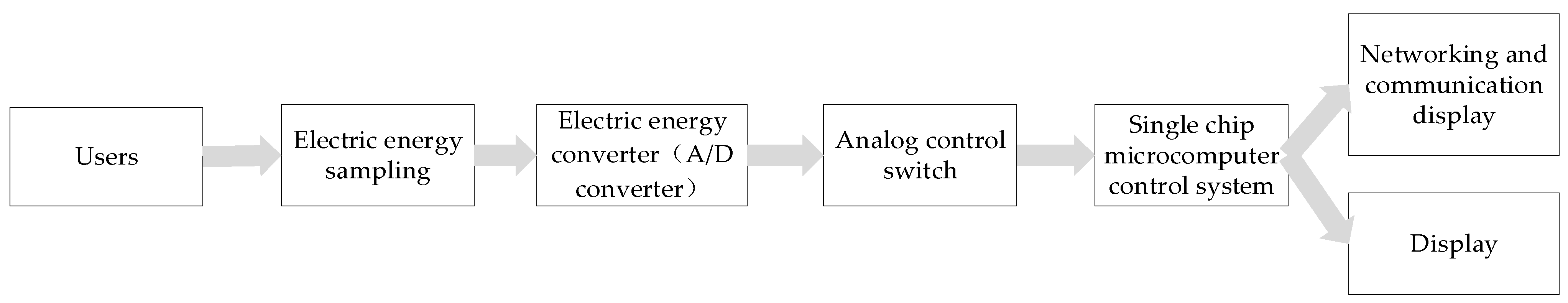
2.1. Introduction of the Working Principle
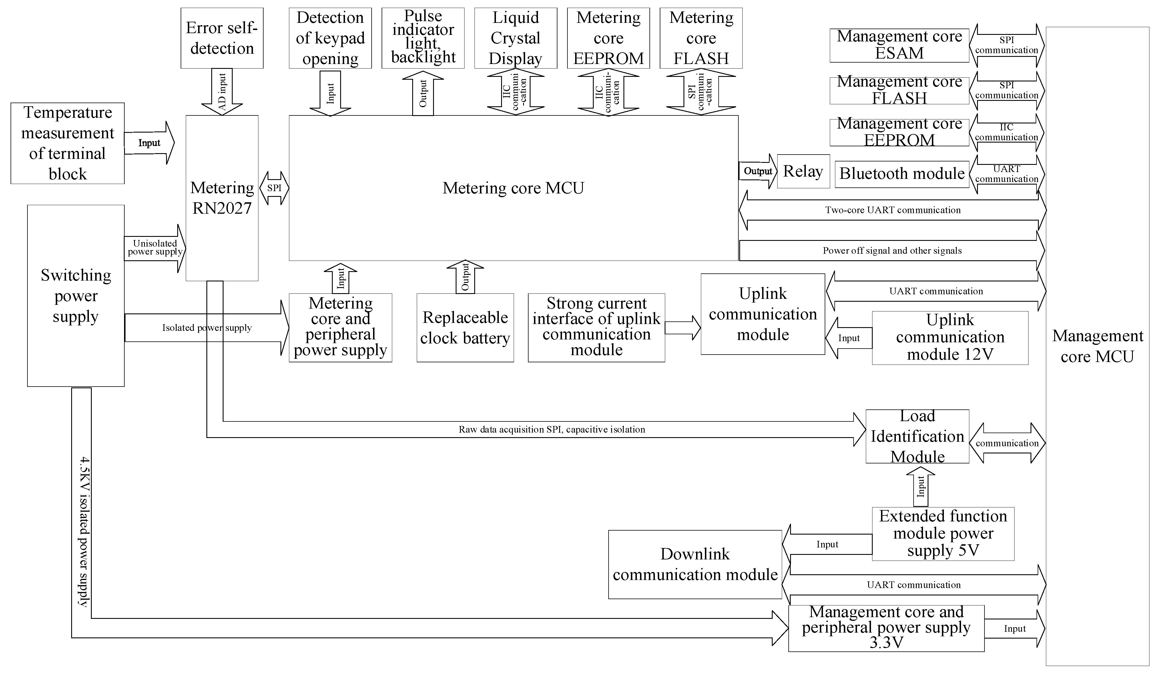
2.2. System Block Diagram and Unit Division
- Power supply unit: The power supply of single-phase smart meter includes AC power supply and low power consumption power supply. AC power supply is the input of the meter, 220 V AC. The power circuit converts 220 V AC into DC at different amplitudes, which is used to power other modules as well as input to the metering module; the low power supply is a lithium battery, which is used as a backup power supply, used to maintain the meter in the event of a power failure.
- Metering core unit: The metering core provides the data of power, clock and so on, and keeps the historical data of forward and backward active power total energy every minute, forward and backward active fundamental energy every 15 min, and forward and backward active power harmonic total energy for electric quantity tracing. The charge and clock of the management core are based on the metering core and synchronized in real time. Metering core can record management core plug, power off, meter reset, calibration, management core upgrade and other event records.
- Management core unit: Management Core is responsible for the whole smart meter management tasks, including fee control, display, communication, event records, data freezing, load control, etc.
- Storage unit: Store all kinds of data generated by the smart meter. When the state of the system changes, all the changed parameters can be written to the memory.
- Communication unit: The communication unit includes uplink communication module, downlink communication module, extended function module and blue tooth communication module to realize the communication function and to read meters and send instructions, etc.
- Display unit: The main display mode of the smart meter is the light emitting diode and liquid crystal. The light emitting diode is mainly the role of the indicator light; the liquid crystal circuit is used to display various types of parameters of the smart meter.
3. Reliability Allocation Method Base on DEA and DBN
3.1. Brief Introduction of Methods
3.1.1. Brief Introduction of the GO Methodology Principle
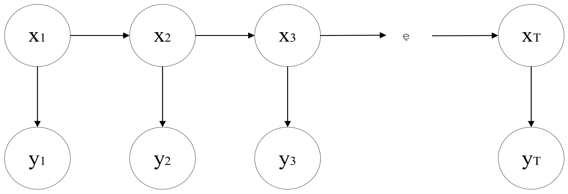
3.1.2. Brief Introduction of the DBN Principle
3.1.3. Brief Introduction to the Principle of Data Envelopment Analysis
3.2. Mapping Rule from the GO Methodology to Dynamic Bayesian Network
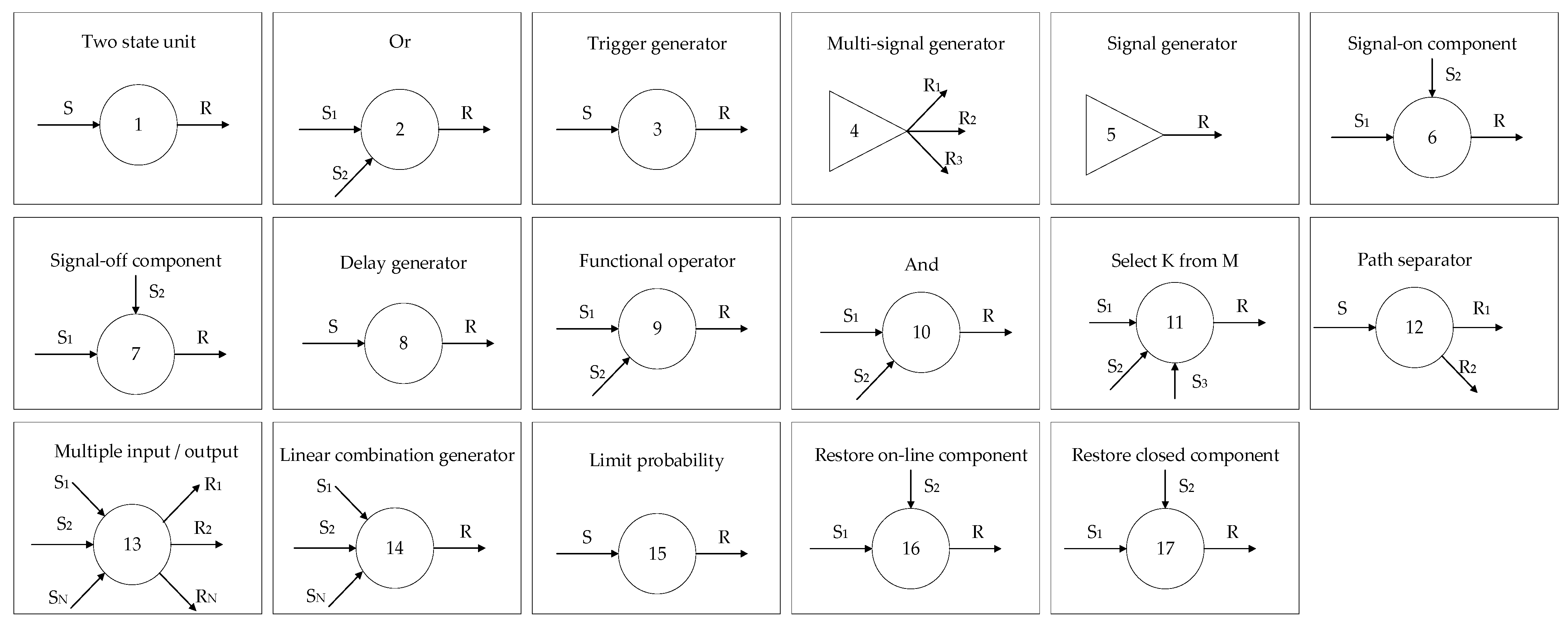
- Operators 1 (two-state unit): Simulation of only two states of the unit (success or failure). When the unit is working, the input signal can go through and there will be an output signal; when the unit fails, the input signal cannot go through and there is no output.
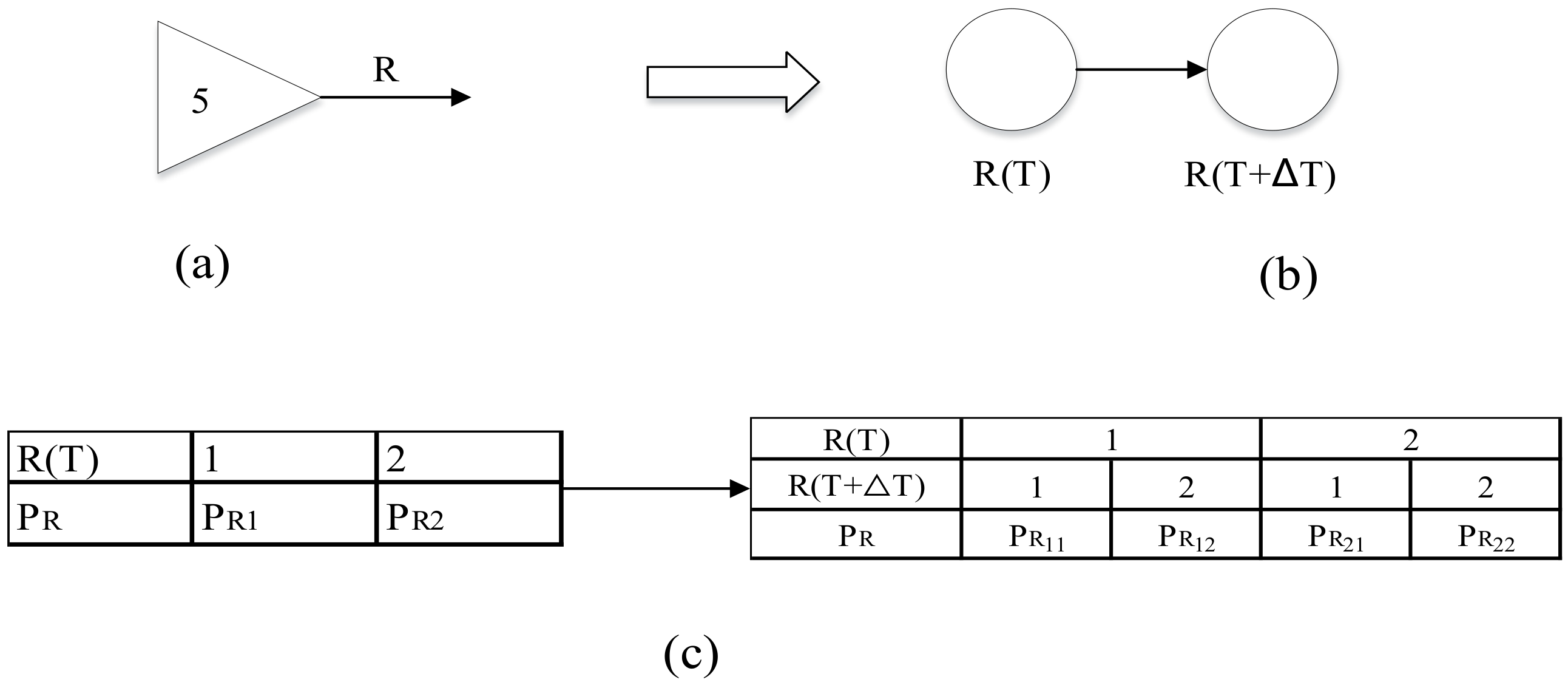
- Operators 5 (signal generator): As an input of the system, analog power supply, water source, generator, etc.
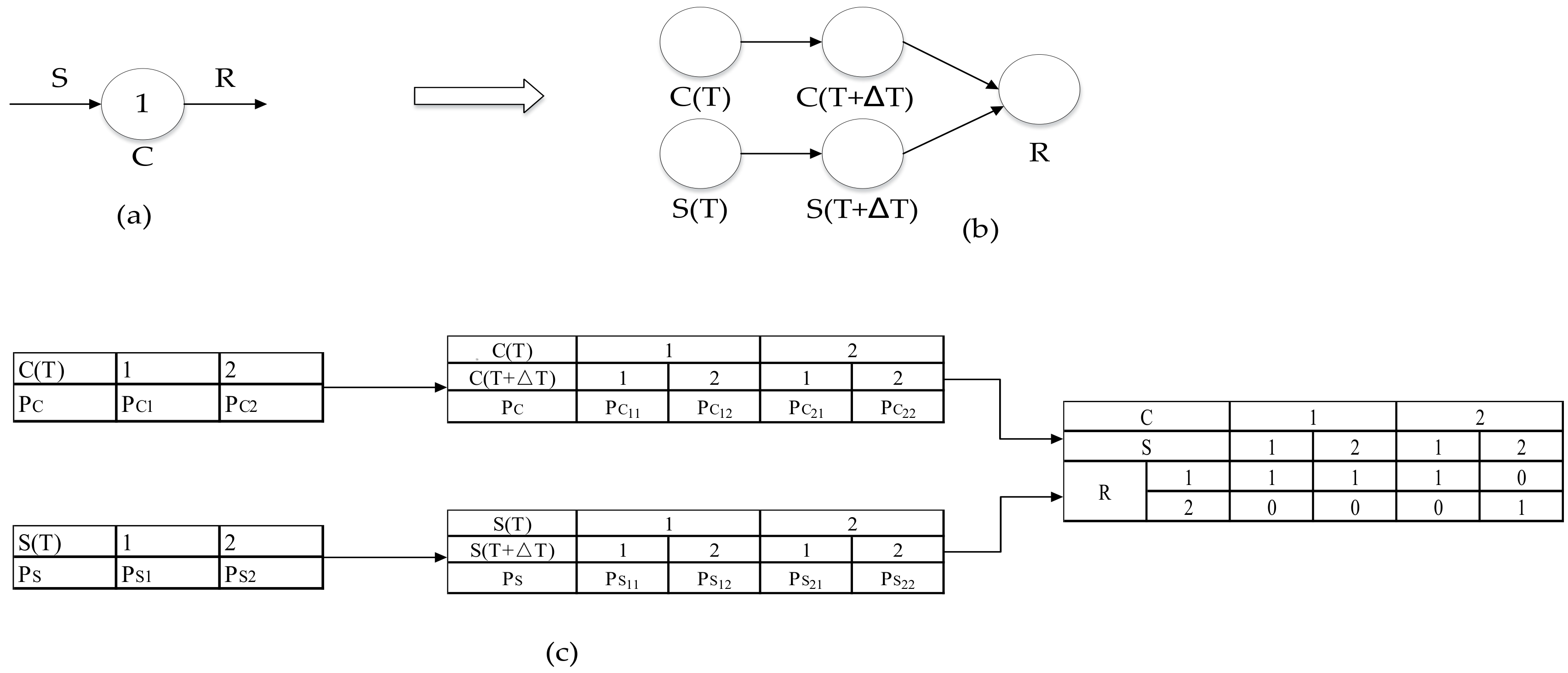
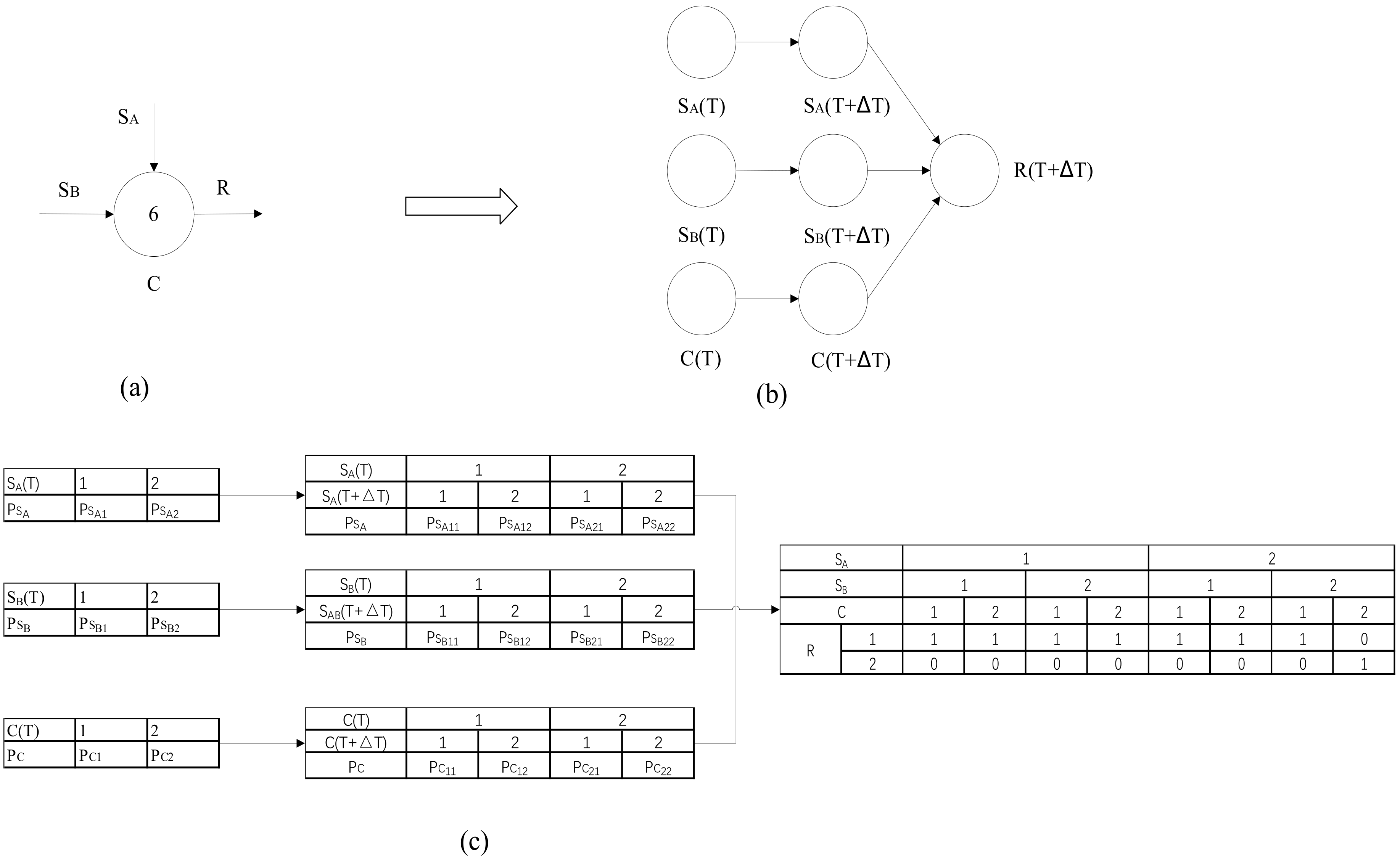
- Operator 6 (signal-on component): A component that requires two inputs to have an output signal.
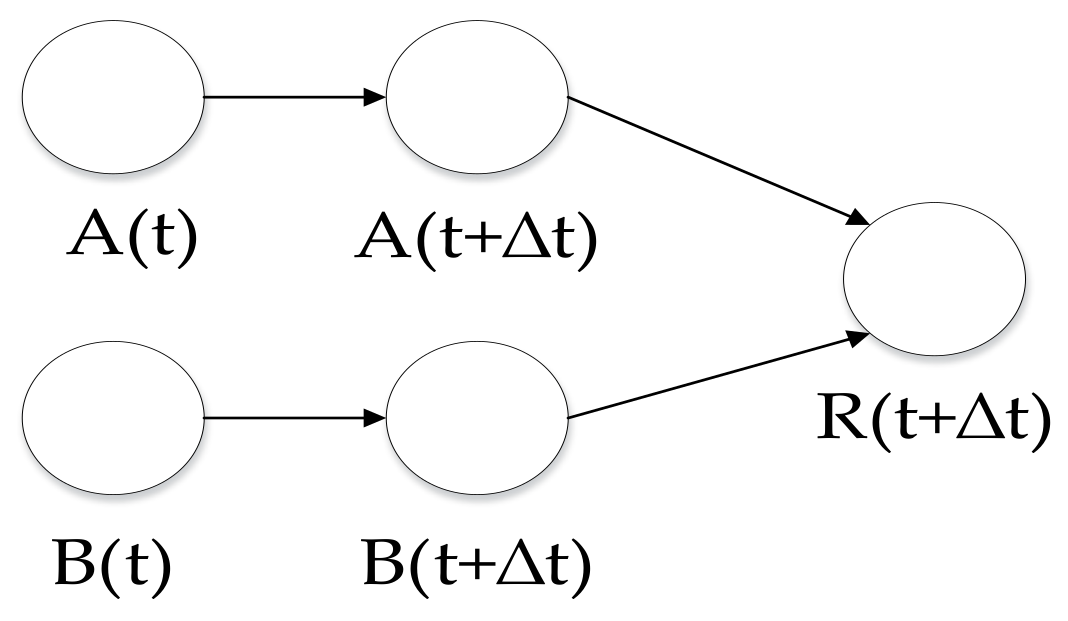
- Operator 10 (and): Multiple input and one output; only if all input signals are successful will there will be an output signal.
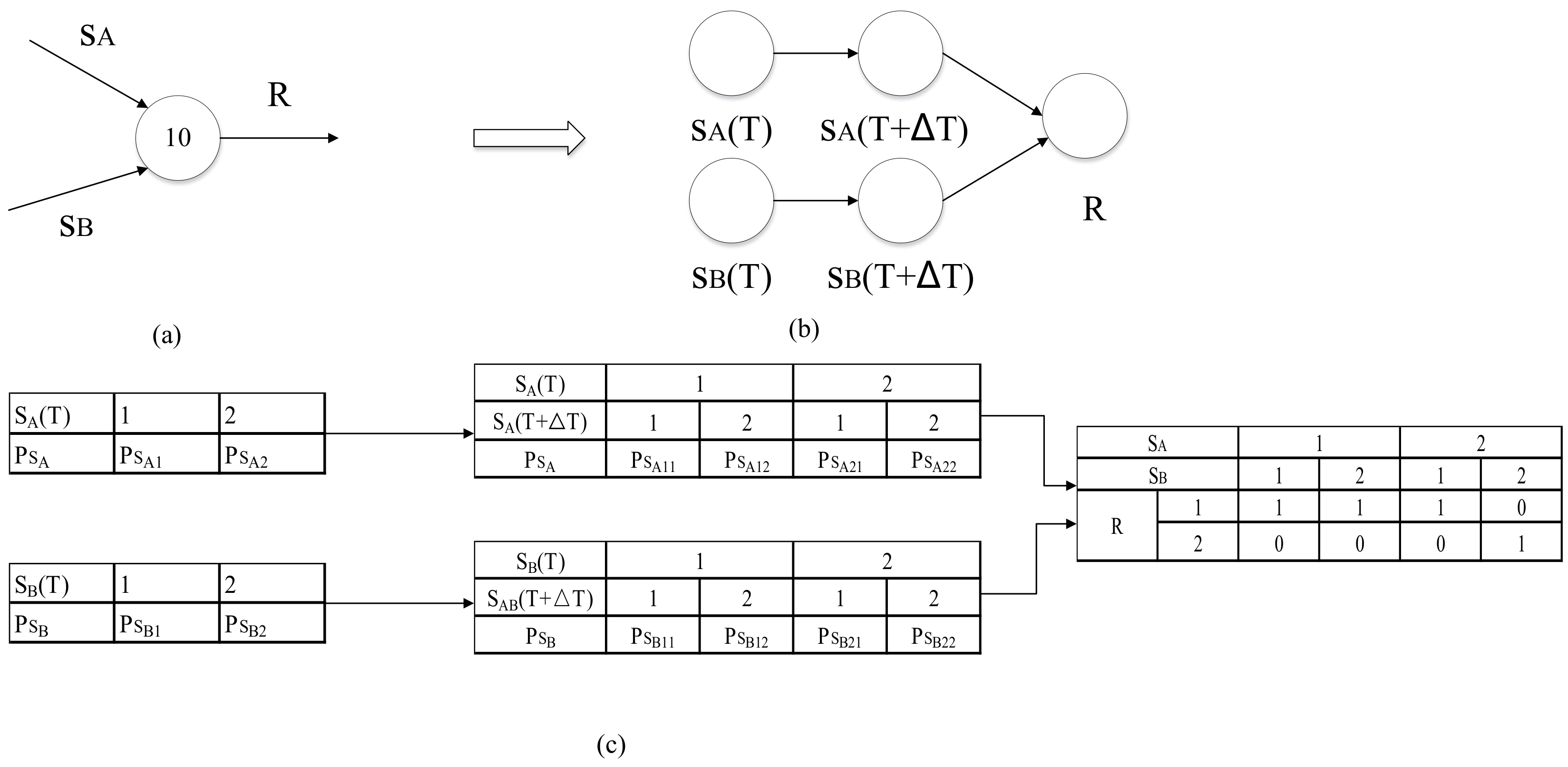
- The nonlogical operator and its input signal flow are mapped to the initial network root node of the dynamic Bayesian network, and the transition network child nodes of each root node are established at the same time. The arrow points from the parent node in the initial network to the corresponding child node in the transition network.
- Each output signal flow except the fifth operator is mapped to a node of the transfer network, and the parent–child connection relationship with all nodes in the transfer network in step 1 is established.
- The prior probability of the root node of the initial network and the conditional probability table (transition probability) of the corresponding child node of the transition network are determined.
- The conditional probability table of the child nodes of the transfer network corresponding to all the output signal flow is given.
3.3. Specific Steps for Reliability Allocation
3.3.1. Division of Units
3.3.2. Backward Reasoning of Dynamic Bayesian Networks
3.3.3. Analysis of Factors Affecting System Reliability
3.3.4. Establishment of the DEA Reliability Allocation Model
3.3.5. Calculation of the Reliability Allocation Weight of Each Unit
3.3.6. Calculation of Reliability after Allocation
4. Reliability Allocation of the Smart Meter
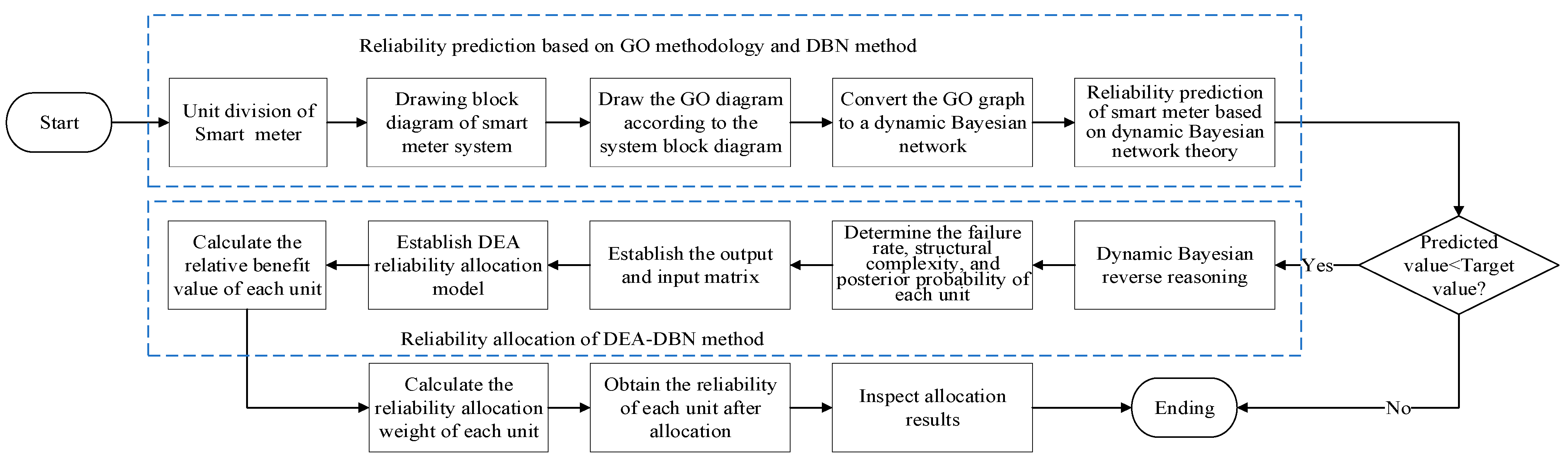
4.1. Reliability Prediction
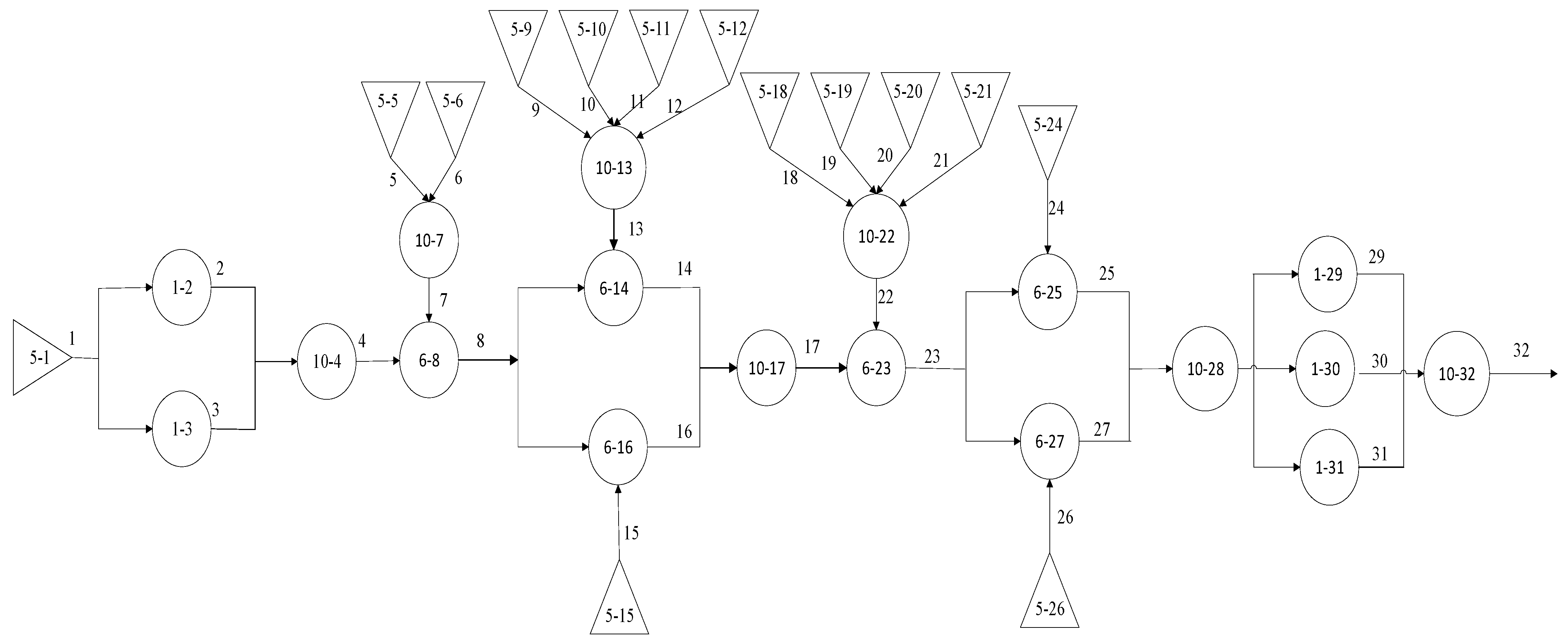
4.1.1. Creation of a GO Diagram for the Smart Meter

| Unit | Component Name | Number | Operator Type | Failure Rate (Fit) |
|---|---|---|---|---|
| power supply unit | Switch power supply | 1 | 5 | 70 |
| Metering core and peripheral power supply | 2 | 1 | 15 | |
| Management core peripheral power supply | 3 | 1 | 15 | |
| Expansion function model power supply | 15 | 5 | 15 | |
| Uplink communication model power supply | 24 | 5 | 28 | |
| metering core unit | Temperature measurement of terminal block | 5 | 5 | 18 |
| Error self-detection | 6 | 5 | 16 | |
| Measurement of RN2027 | 8 | 6 | 25 | |
| Replaceable clock battery | 9 | 5 | 20 | |
| Detection of keypad opening | 10 | 5 | 18 | |
| Metering core FLASH | 12 | 5 | 30 | |
| Metering core MCU | 14 | 6 | 53 | |
| Relay | 28 | 1 | 15 | |
| management core unit | Management core ESAM | 18 | 5 | 10 |
| Management core FLASH | 19 | 5 | 30 | |
| Bluetooth model | 21 | 5 | 20 | |
| Management core MCU | 23 | 6 | 48 | |
| storage unit | Metering core EEPROM | 11 | 5 | 15 |
| Management core EEPROM | 20 | 5 | 10 | |
| communication unit | Load identification model | 16 | 6 | 24 |
| Uplink communication model | 25 | 6 | 35 | |
| Downlink communication model | 26 | 6 | 40 | |
| display unit | Pulse indicator light, backlight | 29 | 1 | 3 |
| LCD display | 30 | 1 | 10 |
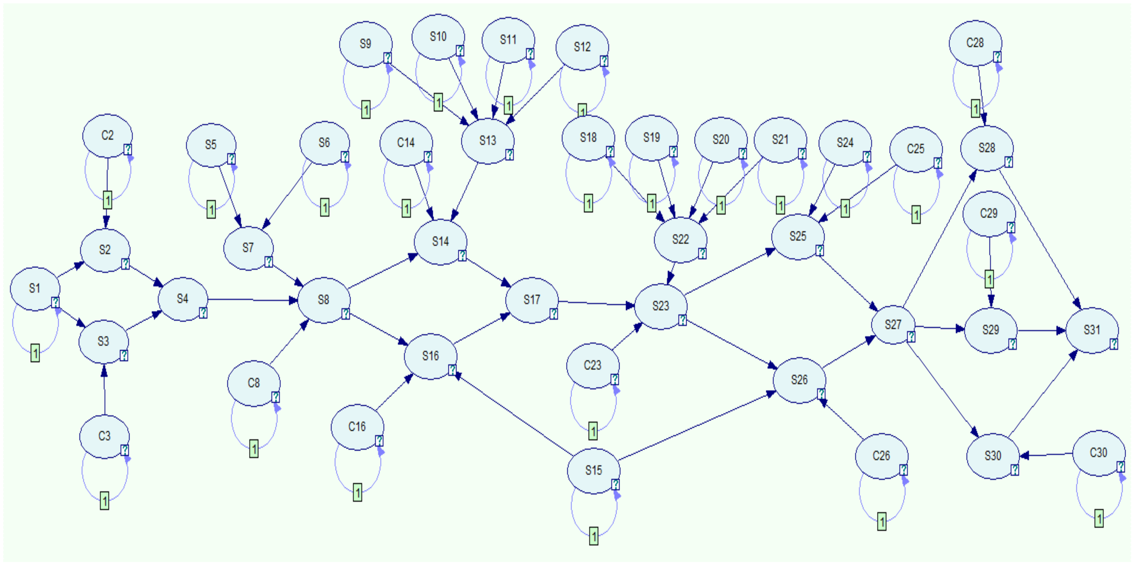
4.1.2. Conversion of the GO Diagram to a Dynamic Bayesian Network
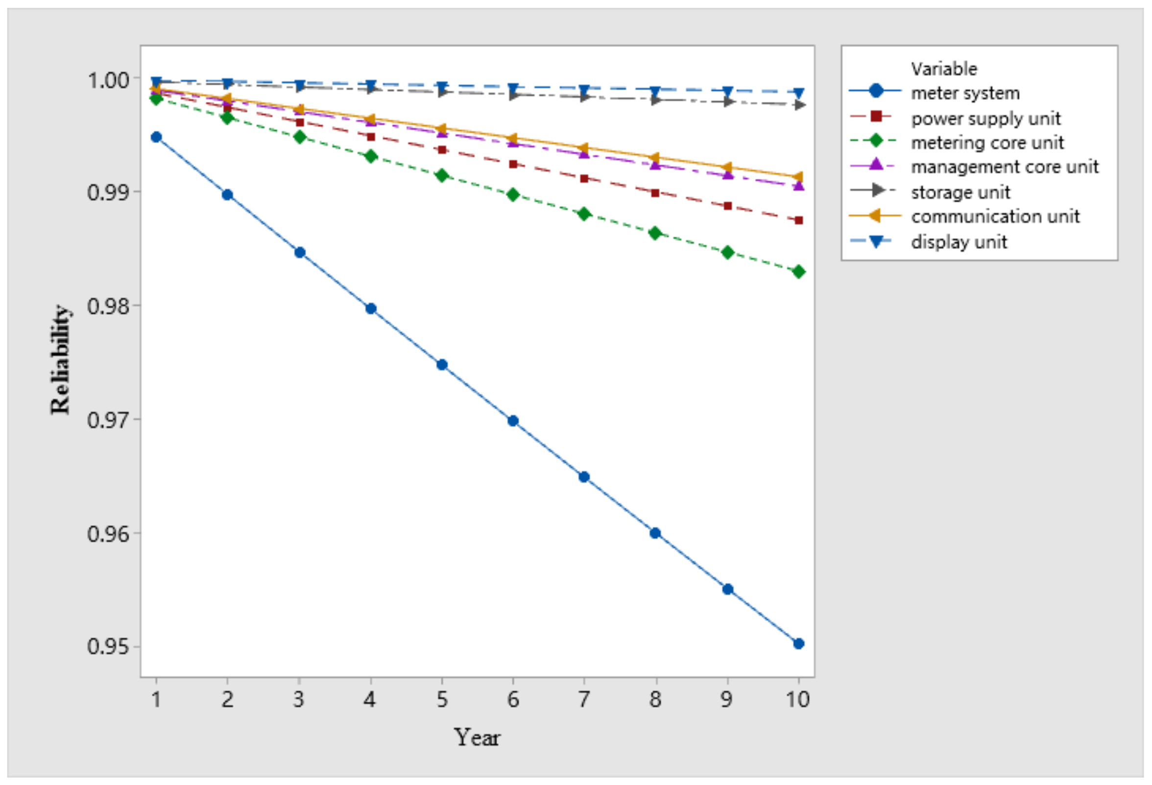
4.1.3. Prediction Results
4.2. Reliability Allocation
5. Verification of Allocation Results
6. Conclusions
Author Contributions
Funding
Institutional Review Board Statement
Informed Consent Statement
Data Availability Statement
Conflicts of Interest
References
- Ou, X.Y.; Zeng, Y.S.; Rang, X.H. IR46 Reliability design and test research of software in smart meters based on IR46. Electr. Meas. Instrumnenation 2019, 56, 147–152. [Google Scholar] [CrossRef]
- Ju, H.J.; Guo, L.J.; Liu, Y.Q. Intelligent Electric Energy Meter Reliability Prediction Research and Application Based on the Component Stress Method. Electr. Meas. Instrumnenation 2013, 50, 7–15. [Google Scholar]
- Han, L.; Li, R.; Xian, H.Z. Reliability Increase Application for Electricity Energy Meters Based on Failure Mechanism. Bull. Sci. Technol. 2017, 33, 193–196. [Google Scholar] [CrossRef]
- Chen, J.T.; Zhu, B.R.; Zhang, Y. Research on the accelerated degradation test scheme of smart meter. Electr. Meas. Instrumnenation 2018, 55, 104–108. [Google Scholar]
- Mellal, M.A.; Zio, E. System reliability-redundancy optimization with cold-standby strategy by an enhanced nest cuckoo optimization algorithm. Reliab. Eng. Syst. Saf. 2020, 201, 106973. [Google Scholar] [CrossRef]
- Yeh, C.T.; Fiondella, L.; Chang, P.C. Cost-oriented component redundancy allocation for a communication system subject to correlated failures and a transmission reliability threshold. Proc. Inst. Mech. Eng. Part O-J. Risk Reliab. 2018, 232, 248–261. [Google Scholar] [CrossRef]
- Zhang, G.B.; Yang, X.Y.; Li, D.Y. Reliability Allocation of Synthetic Assessment Combined with Grey System Theory. Mech. Sci. Technol. Aerosp. Eng. 2016, 35, 906–912. [Google Scholar] [CrossRef]
- Sun, T.; Sun, W.L.; He, L.Y. Research on reliability optimization allocation method of wind turbine based on genetic algorithm. Renew. Energy Resour. 2016, 34, 699–704. [Google Scholar] [CrossRef]
- Ju, P.H.; Jiang, D.X.; Ran, Y. The application of FTA and ANN in reliability reallocation. J. Chongqing Univ. 2018, 41, 11–19. [Google Scholar]
- Yang, Z.; Zhu, Y.P.; Zhang, Y.M. A Comprehensive Reliability Allocation Method for Numerical-controlled Lathes Based on Copula Function. Acta Armamentarii 2016, 37, 131–140. [Google Scholar]
- Wang, B.S.; Yin, J.Y.; Hu, S.S. Research on reliability allocation technology of smart meter based on analytic hierarchy process and group decision-making. Electr. Meas. Instrumnenation 2020, 1–7. [Google Scholar]
- Zhang, H.; Wang, X.B. Data envelopment analysis was used to evaluate green manufacturing process. Acta Armamentarii 2005, 4, 523–527. [Google Scholar]
- Yin, Q.R.; Su, N. Debris-flow risk assessment based on DEA redundancy analysis. Chin. J. Geol. Hazard Control. 2020, 31, 30–34. [Google Scholar] [CrossRef]
- Fang, J.; Ji, W.X.; Song, C.X. Research on the green evaluation decision of elevator parts machinery processing technology. Mod. Manuf. Eng. 2018, 9, 38–43. [Google Scholar] [CrossRef]
- Rashidi, K.; Cullinane, K. A comparison of fuzzy DEA and fuzzy TOPSIS in sustainable supplier selection: Implications for sourcing strategy. Expert Syst. Appl. 2019, 121, 266–281. [Google Scholar] [CrossRef]
- Shen, Z.P.; Huang, X.R. Principle and Application of GO Methodology—A System Reliability Analysis Methodology; Tsing Hua Press: Beijing, China, 2004; pp. 1–8. [Google Scholar]
- Wu, G.H.; Tan, L.; Wei, Z.W. Reliability analysis of regional computer interlocking system based on dynamic Bayesian network. J. Chongqing Univ. 2020, 43, 113–122. [Google Scholar] [CrossRef]
- Tang, Z.; Gao, X.G. Research on Radiant Point Identification Based on Discrete Dynamic Bayesian Network. J. Syst. Simul. 2009, 21, 117–120. [Google Scholar]
- Scutari, M. Bayesian network models for incomplete and dynamic data. Stat. Neerl. 2020, 74, 397–419. [Google Scholar] [CrossRef]
- Jang, L.; Wang, X.M.; Liu, Y.L. DBN-based Operational Reliability and Availability Evaluation of CTCS3-300T Onboard System. J. China Railw. Soc. 2020, 42, 85–92. [Google Scholar] [CrossRef]
- Shen, Z.P.; Gao, J.; Huang, X.R. A new quantification algorithm for the GO methodology. Reliab. Eng. Syst. Saf. 2000, 67, 241–247. [Google Scholar] [CrossRef]
- Shen, Z.P.; Gao, J. GO methodology principle and improved quantitative analysis method. J. Tsinghua Univ. Nat. Sci. Ed. 1999, 6, 16–20. [Google Scholar] [CrossRef]
- Shen, Z.P.; Zheng, T. Exact algorithm for complex system eliability using the GO methodology. J. Tsinghua Univ. Nat. Sci. Ed. 2002, 5, 569–572. [Google Scholar] [CrossRef]
- Motzek, A.; Moller, R. Indirect Causes in Dynamic Bayesian Networks Revisited. J. Artif. Intell. Res. 2017, 59, 1–58. [Google Scholar] [CrossRef]
- Foulliaron, J.; Bouillaut, L.; Aknin, P. A dynamic Bayesian network approach for prognosis computations on discrete state systems. Proc. Inst. Mech. Eng. Part O-J. Risk Reliab. 2017, 231, 516–533. [Google Scholar] [CrossRef] [Green Version]
- Gao, J.L. Research on Reliability of Uncertain Multi-State System Based on Dynamic Bayesian Network. Master’s Thesis, Xidian University, Xian, China, 2019. [CrossRef]
- Martin-gamboa, M.; Iribarren, D.; Garcia-gusano, D. A review of life-cycle approaches coupled with data envelopment analysis within multi-criteria decision analysis for sustainability assessment of energy systems. J. Clean. Prod. 2017, 150, 164–174. [Google Scholar] [CrossRef]
- Mardani, A.; Zavadskas, E.K.; Streimikiene, D. A comprehensive review of data envelopment analysis (DEA) approach in energy efficiency. Renew. Sustain. Energy Rev. 2017, 70, 1298–1322. [Google Scholar] [CrossRef]
- Wang, Y.L. Systems Engineering; China Machine Press: Beijing, China, 2017; pp. 144–147. [Google Scholar]
- Fan, D.M.; Ren, Y.; Liu, L.L. Repairable GO model algorithm based on dynamic Bayesian network. J. Beijing Univ. Aeronaut. Astronaut. 2015, 41, 2166–2176. [Google Scholar] [CrossRef]
- Xiao, Q.K.; Gao, S.; Gao, X.G. Theory and Application of Dynamic Bayesian Network Learning; National Defense Industry Press: Beijing, China, 2007; pp. 46–53. [Google Scholar]
- Chen, X.F.; Wang, H.B.; Xu, R.H. Research on reliability prediction of smart meter based on Bayesian network. Electr. Meas. Instrumnenation 2017, 54, 99–104. [Google Scholar]
- Zhang, Y.M.; Jian, C.J.; Huang, X.Z. Reliability allocation of CNC lathe based on edge worth series method and Data Envelopment Analysis. J. Mech. Strength 2016, 38, 69–73. [Google Scholar] [CrossRef]
- Harbin Electric Instrument Research Institute. Single-Phase Smart Meter Technical Specification; China National Standardization Administration Committee: Beijing, China, 2016; Volume Q/GDW364-2016. [Google Scholar]
- China National Standardization Administration Committee. Reliability of Electrical Measuring Equipment Part 311: Accelerated Temperature and Humidity Reliability Test; China National Standardization Administration Committee: Beijing, China, 2017; Volume GBT 17215.9311-2017. [Google Scholar]
- IEC/TC 13. Electricity Metering Equipment-Dependability-Part 31-1 Accelerated Reliability Testing-Elevated Temperature and Humidity; International Electrotechnical Commission: Geneva, Switzerland, 2008; Volume IEC 62059-31-1 Corrigendum 1-2008. [Google Scholar]


| Allocation Methods | Advantages | Disadvantages |
|---|---|---|
| Equal allocation | The calculation process is simple. | No distinction is made between subsystems and engineering practice. |
| Scoring allocation | The allocation process is simple and can overcome the problems such as insufficient reliability data in the initial stage of design. | Too much reliance on expert judgment. |
| Proportional combination | The allocation process is simple and the allocation result has certain accuracy. | It must be based on old products and be restrictive. |
| AGERR allocation method | Considering the complexity, importance, working time and failure relation of the subsystem, the result of allocation is reasonable. | The influence of engineering factors such as technical constraints on reliability allocation results is ignored. |
| Analytic hierarchy process (AHP) | Comprehensive consideration of reliability factors and full use of expert knowledge. | Large amount of calculation, too much reliance on expert judgment, strong subjectivity. |
| Neural networks | The allocation process is fully based on data, so the allocation result is more accurate. | It needs to be combined with other methods such as fault tree, and the trained neural network is uncertain. |
| Genetic algorithm | When solving the reliability allocation model, it has good convergence, high calculation accuracy, less calculation time and high robustness. | When solving large-scale problems, it is easy to fall into local optimum. |
| Dynamic programming | It can be used to solve nonlinear programming problems. | There is a dimension “disaster” problem. Generally, it is difficult to solve the problem with more than three constraints. |
| Node Number | Component Name | t = 1(Year) | |
|---|---|---|---|
| PR(1) | PR(2) | ||
| S1 | Switch power supply | 0.000613 | 0.999387 |
| C2 | Metering core and peripheral power supply | 0.000131 | 0.999869 |
| C3 | Management core peripheral power supply | 0.000131 | 0.999869 |
| S5 | Temperature measurement of terminal block | 0.000158 | 0.999842 |
| S6 | Error self-detection | 0.000140 | 0.999860 |
| C8 | Measurement of RN2027 | 0.000219 | 0.999781 |
| S9 | Replaceable clock battery | 0.000175 | 0.999825 |
| S10 | Detection of keypad opening | 0.000158 | 0.999842 |
| S11 | Metering core EEPROM | 0.000131 | 0.999869 |
| S12 | Metering core FLASH | 0.000263 | 0.999737 |
| C14 | Metering core MCU | 0.000464 | 0.999536 |
| S15 | Expansion function model power supply | 0.000131 | 0.999869 |
| C16 | Load identification model | 0.000210 | 0.999790 |
| S18 | Management core ESAM | 0.000088 | 0.999912 |
| S19 | Management core FLASH | 0.000263 | 0.999737 |
| S20 | Management core EEPROM | 0.000088 | 0.999912 |
| S21 | Bluetooth model | 0.000175 | 0.999825 |
| C23 | Management core MCU | 0.000420 | 0.999580 |
| S24 | Uplink communication model power supply | 0.000245 | 0.999755 |
| C25 | Uplink communication model | 0.000307 | 0.999693 |
| C26 | Downlink communication model | 0.000350 | 0.999650 |
| C28 | Relay | 0.000131 | 0.999869 |
| C29 | Pulse indicator light, backlight | 0.000026 | 0.999974 |
| C30 | LCD display | 0.000088 | 0.999912 |
| Unit | Smart Meter System | Power Supply Unit | Metering Core Unit | Management Core Unit | Storage Unit | Communication Unit | Display Unit | |
|---|---|---|---|---|---|---|---|---|
| Year | ||||||||
| 1 | 0.994907 | 0.99875 | 0.998293 | 0.999054 | 0.999781 | 0.999133 | 0.999886 | |
| 2 | 0.98984 | 0.997501 | 0.996589 | 0.99811 | 0.999562 | 0.998267 | 0.999772 | |
| 3 | 0.984799 | 0.996253 | 0.994888 | 0.997166 | 0.999343 | 0.997402 | 0.999658 | |
| 4 | 0.979784 | 0.995008 | 0.99319 | 0.996223 | 0.999124 | 0.996537 | 0.999544 | |
| 5 | 0.974794 | 0.993763 | 0.991495 | 0.99528 | 0.998906 | 0.995674 | 0.99943 | |
| 6 | 0.96983 | 0.992521 | 0.989803 | 0.994339 | 0.998687 | 0.994811 | 0.999316 | |
| 7 | 0.964891 | 0.99128 | 0.988114 | 0.993399 | 0.998468 | 0.993948 | 0.999202 | |
| 8 | 0.959977 | 0.99004 | 0.986427 | 0.992459 | 0.998249 | 0.993087 | 0.999088 | |
| 9 | 0.955088 | 0.988802 | 0.984744 | 0.991521 | 0.998031 | 0.992226 | 0.998974 | |
| 10 | 0.950224 | 0.987566 | 0.983063 | 0.990583 | 0.997812 | 0.991366 | 0.998861 | |
| Working Years | 1 | 2 | 3 | 4 | 5 | 6 | 7 | 8 | 9 | 10 |
|---|---|---|---|---|---|---|---|---|---|---|
| Allowable failure rate (%) | 0.2 | 0.25 | 0.3 | 0.35 | 0.4 | 0.45 | 0.5 | 0.55 | 0.6 | 0.65 |
| Reliability (%) | 99.8 | 99.55 | 99.25 | 98.90 | 98.50 | 98.05 | 97.55 | 97.00 | 96.40 | 95.75 |
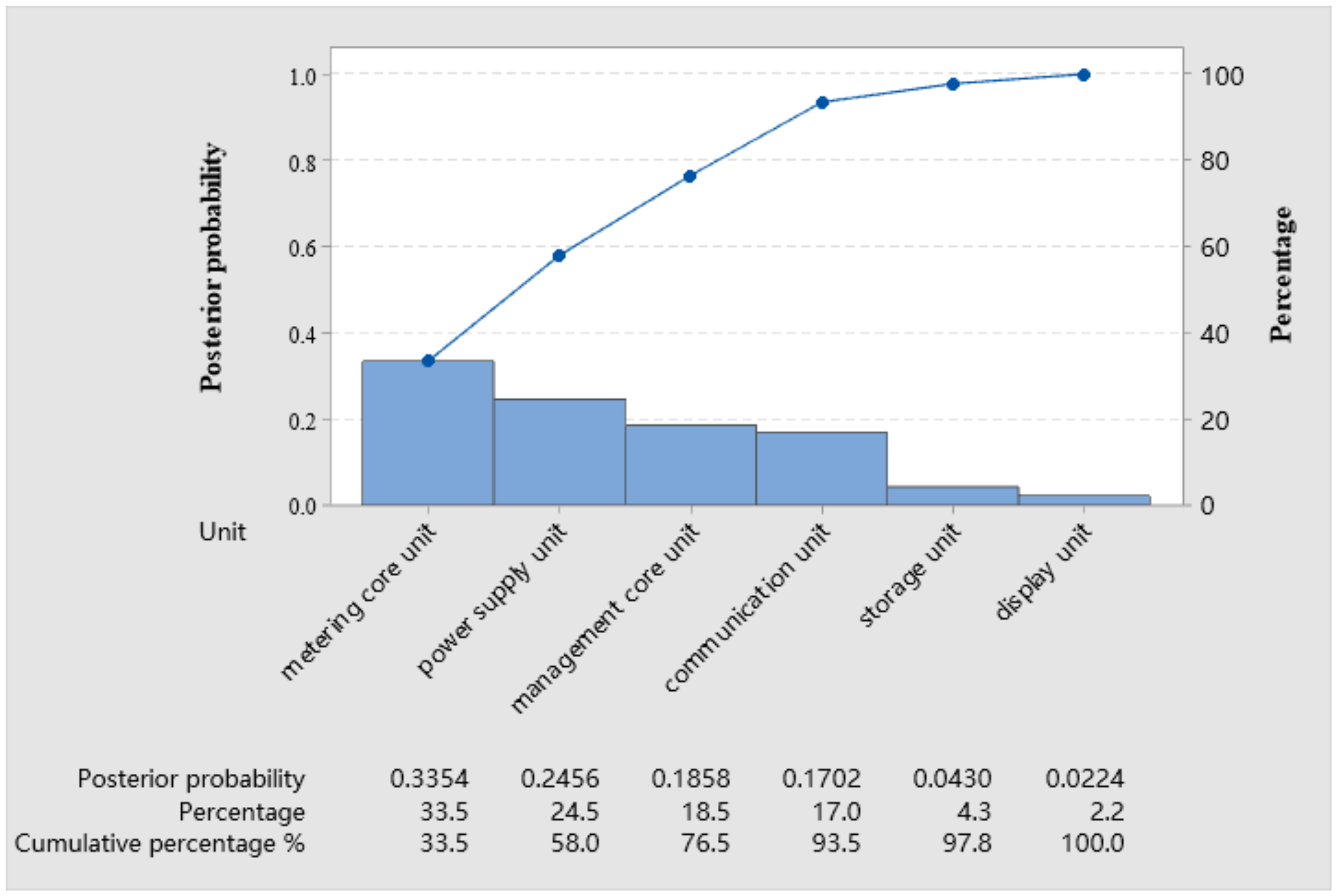
| Number i | Posterior Probability | Failure Rate | Structural Complexity | Value of Input Indicator | |
|---|---|---|---|---|---|
| 0 | Smart meter system | 1.000 | 1.000 | 1.000 | 1.000 |
| 1 | Power supply unit | 0.246 | 0.143 | 0.221 | 1.000 |
| 2 | Metering core unit | 0.335 | 0.195 | 0.286 | 1.000 |
| 3 | Management core unit | 0.186 | 0.108 | 0.195 | 1.000 |
| 4 | Storage unit | 0.043 | 0.025 | 0.065 | 1.000 |
| 5 | Communication unit | 0.170 | 0.099 | 0.143 | 1.000 |
| 6 | Display unit | 0.022 | 0.013 | 0.091 | 1.000 |
| 0 | 1 | 2 | 3 | 4 | 5 | 6 | |
|---|---|---|---|---|---|---|---|
| 1 | 0.614 | 0.604 | 0.656 | 0.672 | 0.144 | 0.264 |
| Unit | 1 | 2 | 3 | 4 | 5 | 6 |
|---|---|---|---|---|---|---|
| 0.614 | 0.604 | 0.656 | 0.672 | 0.144 | 0.264 | |
| 0.208 | 0.204 | 0.222 | 0.227 | 0.049 | 0.089 |
| Working Years | Power Supply Unit | Metering Core Unit | Management Core Unit | Storage Unit | Communication Unit | Display Unit |
|---|---|---|---|---|---|---|
| 1 | 0.999584 | 0.999591 | 0.999556 | 0.999545 | 0.999903 | 0.999821 |
| 2 | 0.999065 | 0.99908 | 0.999001 | 0.998976 | 0.999781 | 0.999598 |
| 3 | 0.998441 | 0.998466 | 0.998334 | 0.998294 | 0.999634 | 0.99933 |
| 4 | 0.997714 | 0.997751 | 0.997557 | 0.997498 | 0.999464 | 0.999017 |
| 5 | 0.996882 | 0.996933 | 0.996669 | 0.996588 | 0.999269 | 0.998659 |
| 6 | 0.995947 | 0.996013 | 0.99567 | 0.995564 | 0.999049 | 0.998257 |
| 7 | 0.994908 | 0.994991 | 0.994559 | 0.994427 | 0.998806 | 0.99781 |
| 8 | 0.993764 | 0.993866 | 0.993338 | 0.993175 | 0.998538 | 0.997319 |
| 9 | 0.992517 | 0.992639 | 0.992005 | 0.99181 | 0.998245 | 0.996783 |
| 10 | 0.991166 | 0.99131 | 0.990562 | 0.990332 | 0.997928 | 0.996202 |
| Year | The First Year | The Second Year | The Third Year | The Fourth Year | The Fifth Year |
|---|---|---|---|---|---|
| Reliability | 0.998002 | 0.995509 | 0.992522 | 0.989049 | 0.98509 |
| Year | The sixth year | The seventh year | The eighth year | The ninth year | The tenth year |
| Reliability | 0.980652 | 0.975741 | 0.970359 | 0.964516 | 0.958219 |
Publisher’s Note: MDPI stays neutral with regard to jurisdictional claims in published maps and institutional affiliations. |
© 2021 by the authors. Licensee MDPI, Basel, Switzerland. This article is an open access article distributed under the terms and conditions of the Creative Commons Attribution (CC BY) license (https://creativecommons.org/licenses/by/4.0/).
Share and Cite
Zhou, J.; Wu, Z.; Yu, Z. Research on the Reliability Allocation Method of Smart Meters Based on DEA and DBN. Appl. Sci. 2021, 11, 6901. https://doi.org/10.3390/app11156901
Zhou J, Wu Z, Yu Z. Research on the Reliability Allocation Method of Smart Meters Based on DEA and DBN. Applied Sciences. 2021; 11(15):6901. https://doi.org/10.3390/app11156901
Chicago/Turabian StyleZhou, Juan, Zonghuan Wu, and Zhonghua Yu. 2021. "Research on the Reliability Allocation Method of Smart Meters Based on DEA and DBN" Applied Sciences 11, no. 15: 6901. https://doi.org/10.3390/app11156901