1. Introduction
Currently, the use of robot arms has dramatically increased in various applications, including manufacturing, logistics, medicine, home, education, defense, and factories. due to their plentiful benefits such as high quality, fast production, less waste, and excellent safety (removing employees from hazardous working conditions, and handling heavy parts).
Because of their crucial role, path planning, including target reaching and obstacle avoidance, is essential. Therefore, this article tries to address the issues of path planning methods to improve the efficiency of their operation. In this regard, since all robot arms’ activities are dependent on their end-effector, target reaching (i.e., getting the end-effector to the desired position) is a crucial task for them. Additionally, obstacle avoidance is another equally vital task for these robots because robot arms must avoid self-collisions and any objects within their workspace.
For the past decades, scholars have presented many algorithms in robot arm path planning to improve those tasks. Artificial Potential Field (APF), Probabilistic Road Maps (PRM), Rapidly exploring Random Tree (RRT), Reinforcement Learning based (RL-based) are some of the well-known examples.
In this regard, some of the authors used the APF method for path planning. Sheng Nan Gai et al. presented a whole-arm path planning algorithm for a 6-DOF industrial robot based on the artificial potential field method [
1]. Hsien-I Lin et al. proposed a path planning method and gave an idea for collision avoidance by a three-dimensional artificial potential field for a robot arm [
2]. However, this method can become trapped in the local minima of the potential field and fail to find a path or find a non-optimal path [
3].
Some other authors used the PRM method for path planning. Zahid Iqbal et al. presented a path planning algorithm for robots based on PRM [
4]. Nevertheless, this approach is time-consuming and requires re-planning when the initial position changes [
3].
Some others presented an RRT algorithm for path planning. Kun Wei et al. proposed a dynamic path planning method for robotic manipulator autonomous obstacle avoidance based on an improved RRT algorithm [
5]. Yuelei Liu et al. proposed an improved RRT algorithm by introducing the random point generation mechanism based on random probability. Nonetheless, this method has many problems, including cubic graphs, irregular paths, and non-optimal paths [
6]. That is because the structural nature of these graphs hinders the probability of finding an optimal path. Additionally, like the PRM, this method is time-consuming and requires re-planning when the initial position changes [
3].
Since the reinforcement learning methods have the advantage of high computational efficiency, some authors used RL-based methods to address path planning limitations. Shuhuan Wen et al. presented a new obstacle avoidance algorithm based on an existing deep reinforcement learning framework called deep deterministic policy gradient (DDPG) [
7]. Evan Prianto et al. proposed a Soft Actor-Critic-based path planning algorithm to overcome RL-based path planning difficulties [
8]. Fangyi Zhang et al. proposed a modular method to efficiently learn and transfer visuomotor policies from simulation to the real world. They combine domain randomization and adaptation. In fact, in that paper, they could generate trajectories to control the arm with a random initial configuration to reach a target arbitrarily placed in the operation area, regardless of obstacle avoidance [
9]. Mengyu Ji et al. used approximate regions instead of accurate measurements to define new state space and joint actions in the Q-learning method [
3]. Nevertheless, some other researchers prefer not to use RL-based methods for solving the robot arm path planning problem because it has to take each joint’s motion into account, which makes them slow and complex.
Other authors presented some unconventional methods, for example, polynomial path planning method. In this method, the end-effector positions can be determined by a polynomial from the start point to the final point. Then, the joints angles can be obtained by using inverse kinematic. Firas S. Hameed et al. presented a real-time path planning method to avoid collision with obstacles for a fixed robot arm that combines the benefits of both global and local techniques. This method is based on the idea of configuring the robot arm to adjust its joints on a selected polynomial to solve the inverse kinematics problem [
10]. Tse-Ching Lai et al. proposed a path planning method to avoid collision with obstacles, based on non-uniform rational B-splines and a smooth polynomial [
11]. However, these methods have many problems, including high computational costs and time-consuming processes because to find the joints angles, the inverse kinematic should be used in each step, which makes the algorithm too slow.
All in all, there are many problems in the methods mentioned above, including failing to find a path, finding a non-optimal path, complexity, time-consuming, requiring re-planning, cubic graphs, irregular paths, and slowness. Since slowness and complexity can negatively affect the performance of robot arms and thus production, finding a new path planning method to address these two limitations is essential. Solving these limitations can significantly reduce the computational cost of robot arms’ path planning. More than this, it can also increase the speed of production, which has many economic benefits for factories. Indeed, the faster production, the more efficient the costs are spent by the company for the production process. For these reasons, in this paper, we present a novel hybrid path planning method based on Q-learning and a neural network to improve the slowness and complexity.
In the proposed approach, we divide the path planning process into two separate phases, active and passive. In the first part, using the Q-learning algorithm and inspired by the “windy grid world” problem, a sequence of simple actions is found in a gridded workspace so that the robot arm begins moving from the start cell to reach the target cell while avoiding collision with an obstacle. In other words, the robot arm learns how to get the target and avoid collision with the obstacle in a simplified agent-environment interaction. A simplified RL problem reduces the complexity and slowness due to using a simple environment, states, and actions. The states are the cells in the gridded workspace, and the actions are moving up, down, left, and right. Although this simplification makes the process fast, the results of this process, such as up, down, left, and right, cannot be used in the robot arm, so the second part is used to find useable actions. In the second part, using a trained neural network, the required angles of the found actions are obtained. It is worth mentioning that it does not need to run a time-consuming neural network process because its weights were already trained; thus, it saves computational time.
The first part, action-finding, is called the active phase because, in this part of the hybrid path planning, a learning code is run, which takes time to learn. In other words, during this part of our hybrid path planning, the robot uses an active section of memory and computer brain that needs to do a learning process, which is a time-consuming process. On the other hand, the second part, angle-finding, is called the passive phase because, in this part of path planning, the neural network does not need to be trained every time; instead, it is trained only one time and is used forever. In other words, during this part of our hybrid path planning, the robot uses a passive section of memory without needing to do any learning or training processes, which are time-consuming. The combination of these two active and passive phases reduces the complexity and improves slowness.
In summary, in this paper, it is hypothesized that dividing the path planning into two separate phases, including active and passive phases, can improve the slowness and complexity of the path planning methods, which are among the two most important issues. This is because using simplified environment, agent, and state-action spaces helps us to avoid linking a simulator with a learning code to perform an agent-environment interaction. Furthermore, using a trained neural network for finding the joints angles helps us to save time before starting the path planning. This is because, unlike the training mode of a neural network which is time-consuming, the using mode takes less time which means time is saved. Therefore, if we use a hybrid method, path planning will be faster and less complex than before.
The paper is organized into four sections. Introduction and background, method and strategies, simulation and experimental results, and conclusion are, respectively, four sections.
2. Method Description
Path planning for robot arms is a computational problem that is defined as finding a sequence of valid joints angles that moves the robot from the start point to the target. Since robot arms contain multi DOF and a large workspace, finding an optimal path is a complex and slow process. Given the presented literature review, according to previous path planning methods, the robot arm had to run a time-consuming algorithm and compute complex calculations that need large memory and a strong computer brain to support such huge calculations. Additionally, a slow process prevents an algorithm from being used in a real-time process. Therefore, to address that, we raise the idea of the hybrid active-passive phases to reduce the load of computation on the robot arm computer brain. In the following sections, we present each component in detail.
2.1. Action-Finding by Q-Learning (Active)
The first component, action-finding, contributes to this study by offering a simple action and state in the Q-learning algorithm. This component of the hybrid path planning is called the active phase because, in this part, a learning code is run, which needs to spend time. In other words, during this part of our hybrid path planning, the robot uses an active section of memory and computer brain that needs to do the learning process, which is a time-consuming process.
Q-learning, which is used in this section, is an off-policy algorithm in RL, which is an area of machine learning concerned with how intelligent agents ought to take actions in an environment to maximize the notion of cumulative reward. An RL agent interacts with its environment in discrete time steps. At each time , the agent receives the current state and reward . It then chooses an action from a set of available actions, which is then subsequently sent to the environment. The environment moves to a new state and the reward associated with the transition (, , ) is determined. The goal of an RL agent is to maximize the expected cumulative reward.
Since this component of our hybrid method uses the Q-learning algorithm, we need to clarify the difference between this part of our method and other RL-based path planning methods. In the traditional RL-based path planning methods, the path, which is a discrete sequence of the joints angles from the start point to the final point, is found via RL algorithms. The goal is to discover the optimal policy maximizing the total reward that the agent gets in path planning iteration. In other words, RL determines how an agent can take a series of actions to maximize cumulative returns. It means that the robot needs to interact with the environment to learn. Yet, interacting with the real world to be trained is highly dangerous and harmful because the robot may hit obstacles and get hurt or damage its environment. Additionally, interacting with a real environment is time-consuming and expensive. Thus, to avoid these damages and costs, scholars usually use a simulator so that the robot arm interacts with the environment. Although using simulators is highly useful, they are relatively complex because learning via interacting with the simulation world needs linking between simulators and learning codes. Additionally, in the traditional RL-based path planning, since the robot arm is a multi-rigid series structure with several degrees of freedom, the rotation of each joint needed to be taken into account as states. This should not be done not only in each iteration but in each action in the sequence of actions of the path. This makes these types of path planning highly complex and slow.
However, in this paper, we use the Q-learning algorithm to find a simplified sequence of actions such as up, down, left, and right instead of joints angles without the need of linking between a simulator and learning code. The action-finding component of our hybrid path planning method is inspired by the “windy grid world” problem. We first divide the 2D workspace into several cells. The number of cells depends upon the resolution. In the original “windy grid world” problem described by Sutton and Barto [
12], the goal is to move from the start cell to the target cell while facing an upward wind in the middle of the grid. In contrast, in this paper, we assume an obstacle in an arbitrary cell, and there is also no wind. Unlike RL-based methods, instead of finding a sequence of joints angles, this method finds a simple sequence of actions, including up, down, left, and right, to move from a cell (state) to its adjacent cells (states). This assumption makes the action-finding process simple and fast because it no longer needs to connect to a simulator for learning; instead, the gridded workspace is simple enough to be used in a learning code as an environment. We can write the state space and action space in the following ways.
where
n and
m are the world width and world length, respectively. In fact, the more resolution it needs, the more cells we should provide. The state space has only
members.
The action space has members, including simple movements of up, down, left, and right.
Since the state space and action space are smaller and more straightforward, interacting with the environment can be modeled in programming software easily without using simulators, which are basically complex software. This strategy can significantly reduce the running time of code and improve complexity.
Before starting the Q-learning algorithm to find the optimal path, we must identify three positions: the position of start, the position of the target, and the obstacle’s position. Like in real applications, we place the position of start, target, and obstacle randomly. Therefore, to detect the positions, an image processing algorithm is used. We use a picture taken by the camera from the top view, which is cropped from the 2D workspace, as input of the image processing section. Indeed, by a computer vision algorithm, five different colors, including yellow, which represents the start point; red, which represents the obstacle; green, which represents the target; black, which represents grid borders; and white, which represents background color, are detected via their RGB code. Then, it is ready to use the KNN algorithm for further analysis. KNN is one of the simplest classification algorithms available for supervised learning. This algorithm falls under the supervised learning category and is used for classification (most commonly) and regression. It is a versatile algorithm also used for imputing missing values and resampling datasets. As the name (K Nearest Neighbor) suggests, it considers K Nearest Neighbors (data points) to predict the class or continuous value for the new data point [
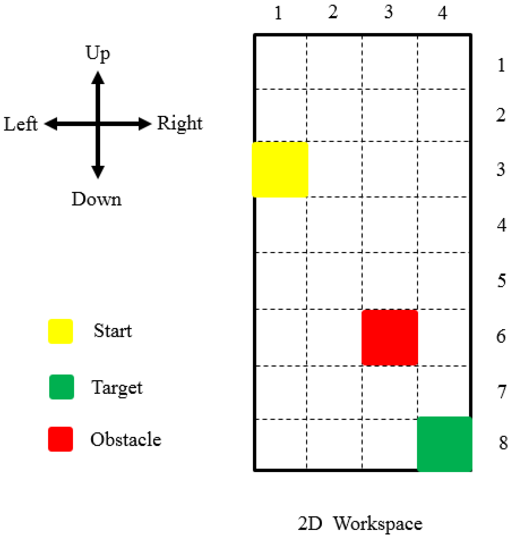
13]. By means of the KNN algorithm, we classify pixels of the images by different colors via RGB code of colors to differentiate between the start cell in yellow, the obstacle cell in red, the target cell in green, and the rest of the cells in the background color. The idea is to search for the closest match of the RGB code of colors of pixels. So, since there are five main colors, including yellow, red, green, black, and white, we use an optimum number for the K. In this section, the image pixels are swept so that the coordinate of the center of each particular color is obtained. Thus, in order to increase the speed of sweeping, a low-resolution image can be used. Simply put, the KNN algorithm classifies unknown pixel points by finding the most common class among the K-closest examples. We defined a distance metric or similarity function by pixels indexes of the image to apply the KNN classification. This simple algorithm is used to avoid complexity. In other words, we use this algorithm because the KNN classifier is by far the simplest machine learning and image classification algorithm. In fact, it is so simple, and it does not need to be trained. However, this algorithm has a few limitations: since KNN finds coordinates of pixels with similar colors, start, obstacle, and target cells have to have different colors. Additionally, we can only use one obstacle unless we use different colors for obstacles. In fact, although the KNN is simple and faster than other algorithms, it is not able to distinguish objects by their shape, but it can detect them by their colors. All in all, KNN image processing distinguishes the start, target, and obstacle from other areas, and then it obtains their coordinates of the center of the area by analyzing the picture taken from the top view of the 2D workspace. It should be noted that a workspace of a robot arm is the set of all positions that it can reach. This depends on several factors, including the arm’s dimensions, number of joints. However, in this method, the 2D workspace is a fraction of the whole workspace active in the production line, which is highly common in factories. Where robot arms are fixed and placed next to a conveyor belt and do assembly process or manufacturing process. In
Figure 1, a scheme of the 2D workspace with three main cells, including the start in yellow, target in green, the obstacle in red, and direction of actions, are shown from the top view.
As
Figure 1 shows, in this paper, we choose four actions, including up, down, left, and right as action space. Although it is possible to increase the number of actions, the computational cost will increase as well. Additionally, the resolution, which is actually the size of end-effector motion in each step, can be increased but at the cost of a higher computational load. It is also possible to decrease it but at the risk of finding no path. Indeed, there is a trade-off in the granularity of discretization or resolution: too fine will increase the search space exponentially, result in greater computational cost and slowness, and too coarse may result in failing to find a path even if there exists one or finding inaccurate results. In the results section, we will show the resolution effect on slowness by providing the diagram of Q-learning, neural network, and total running time versus the number of cells. As the number of cells increases, the time of running Q-learning code increases too. According to the application of the robot arm, one should determine that what resolution and speed are suitable. In this article, according to the required resolution and speed, we use an eight-by-four gridded 2D workspace that means there are thirty-two cells (states) in which the end-effector can be placed. The cells in which the start, target, and obstacle are located are considered the start, target, and obstacle cells, respectively. Then, the best actions from the start cell to the target cell are found by the Q-learning algorithm under reward and punishment conditions.
We use Q-learning as the RL algorithm because, according to Seijen’s results [
14], to get a maximum accumulated reward in windy grid world and maze problems, the Q-learning algorithm is better than the SARSA and other algorithms. In other words, since our problem is similar to Seijen’s problem, we use Q-learning as the RL algorithm in the action-finding phase. Q-learning is an off-policy RL algorithm that seeks to find the best action to take given the current state. It is considered off-policy because the Q-learning function learns from actions that are outside the current policy, like taking random actions, and therefore a policy is not needed. More specifically, Q-learning seeks to learn a policy that maximizes the total reward. In this method, the reward and punishment are defined as follows: the agent receives a reward +50 if it reaches the target cell. The agent gets a punishment of −100 if it reaches the obstacle cell. Finally, all other actions result in −1 punishment. Given these roles, the agent tries to reach the target to earn and collect the maximum reward. Additionally, the agent tries to avoid obstacles and other useless actions to collect maximum rewards. It can be said that the Q-learning algorithm starts searching the optimal sequence of actions from the start cell and then reaches the target cell while avoiding the obstacle cell. In this article, the gridded 2D workspace has the following configuration and rules:
The gridded 2D workspace is 8-by-4 and bounded by borders, with four possible actions including up, down, left, and right;
The agent begins from the start cell, which is randomly located in a cell;
The agent receives a reward of +50 if it reaches the target cell which is randomly located in a cell;
The agent receives a punishment of −100 if it reaches the obstacle cell which is randomly located in a cell;
All other actions result in −1 punishment.
By following the Q-learning algorithm, the best actions that the robot can do in any state (cell) to reach the target and avoid the obstacle are determined. Having a matrix of the best actions that the robot arm can do in each cell is the aim of the action-finding section.
2.2. Angle-Finding by Trained Neural Network (Passive)
The second component, angle-finding, provides joints angles of each selected action in a particular cell by a trained neural network. In other words, after finding the appropriate actions in the action-finding section, it is time to obtain the joints angles for each selected action in each cell to be understandable for the robot arm. This component of our hybrid path planning is called the passive phase because we use a trained neural network, which is a static process in contrast to a dynamic process like Q-learning. In other words, the neural network does not need to be trained every time; instead, it is trained only one time, but that trained neural network is used every time during path planning. Indeed, during this part of our hybrid path planning, the robot uses the passive section of memory without needing to do any learning or training processes, which are time-consuming.
Before definition the type of neural network used in this paper, it is better to discuss other angle-finding methods because it can help to understand the advantages of using neural networks. One of the most common approaches in the classic methods to find joints angles is inverse kinematics (IK). The idea behind IK is to calculate the joints angles of the robot arm for a given position of the end-effector. To accomplish motion with this approach, one would first compute a path for the end-effector from the initial position to the target position. Then, with IK, the joint configurations needed for each intermediate time step along the trajectory are calculated. However, using IK in each step makes the method extremely slow. Considering the article’s aims, which are improving slowness and improving complexity, the IK is not a suitable one due to its slowness.
Another way of angle-finding is to use table lookup. In this method, a table containing states in its rows, actions in its columns, and angles in its heights is used. Nonetheless, this method is still inefficient because, in high resolution of moving (i.e., more cells), a large table should be provided and saved. It is blatantly apparent that using a large table can make the method slow, which slowness is out of the aim of this article.
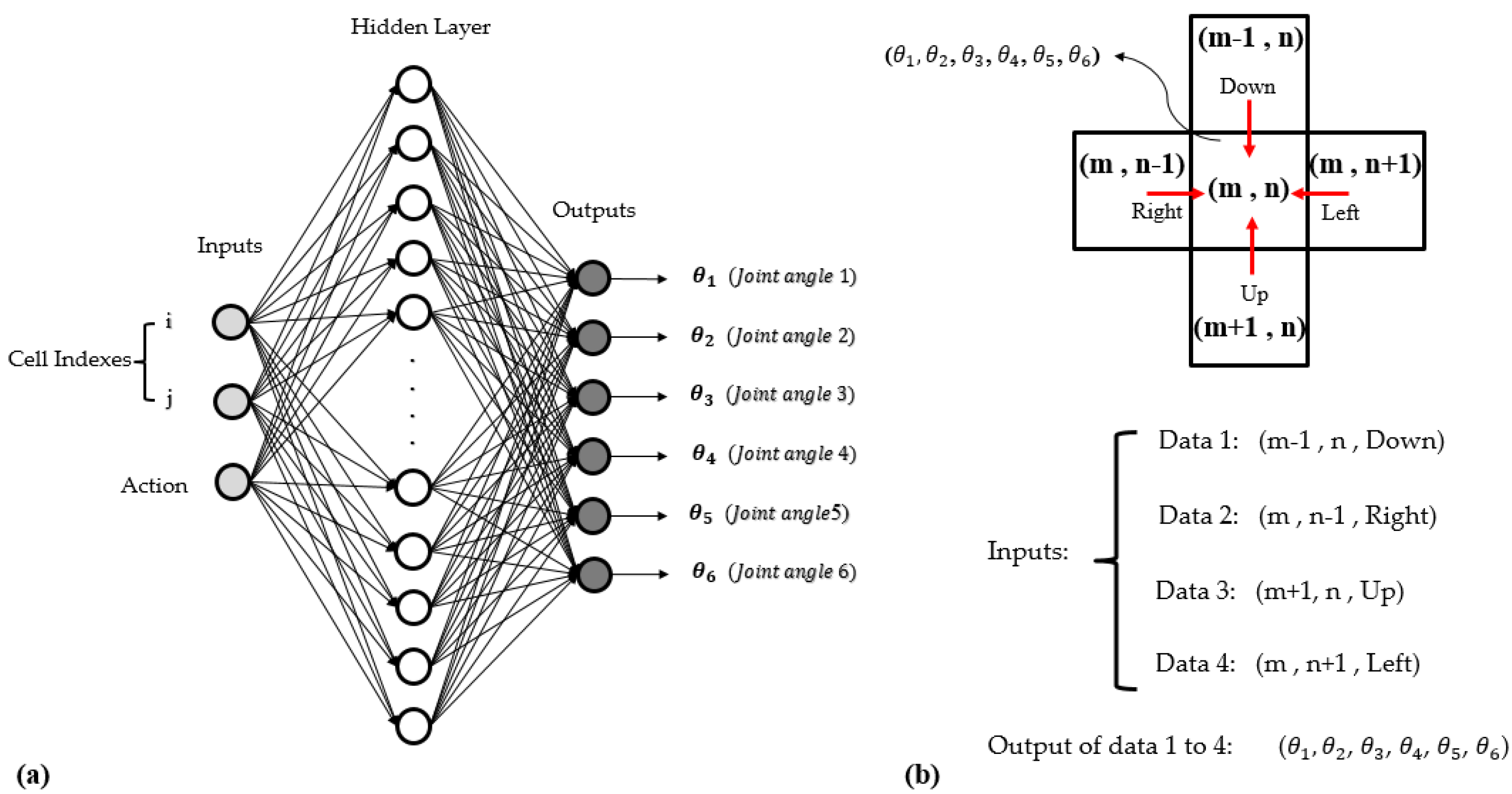
Given the disadvantages of IK and table lookup methods presented in previous paragraphs, we use a neural network in the angle-finding phase. In this paper, we train a neural network to use in the angle-finding section. The proposed neural network is trained by using a data set. A data set usually is collected by a real robot in experimental environments. Yet, in the cases that a robot arm there exists in the simulator’s library, one can use simulator software to collect data. However, it should be noted that for high resolution of the grid, in which the distance between cells is small, using the real robot in experimental environments is recommended because the error between the simulator and the real robot is no longer ignorable. In this paper, we collected the data by means of the RoboDK simulator because our robot arm exists in the RoboDK library, and also our resolution of the grid is relatively low. Since required joints angles of moving toward each direction are dependent on the current state of the end-effector, in each step, that current cell must be taken into account in the neural network. Therefore, the indexes of the cell’s row and column and the selected action should be the inputs of the neural network, and then the joints angles that provide the position of the next cell corresponding to the action are its outputs. It is worth mention that since the input must be in numerical form, the actions including up, down, left, and right are rewritten numerically as 1, 2, 3, and 4, respectively. Moreover, the number of outputs is dependent on the degree of freedom of the robot arm. In a robot arm which have six joints, the number of outputs is equal to six.
The neural network structure we propose has one hidden layer, which has thirty neurons. The number of hidden layers and their neurons was selected empirically by trial and error during the training. It also has three inputs, including indexes of the row and column of the current cell and selected action. It has six outputs because the robot arm used in this article is model IRB 1600 that is a 6 DOF type. The activation functions of the input and output neurons are the ReLU (Rectified Linear Unit) function because this function is most widely simply used without any complexity. Additionally, the activation function of the hidden neurons is the sigmoid function.
After designing the overall structure of the neural network, we collect data set to train it with respect to the designed structure. In order to collect the data set, we place the end-effector of the robot arm in different cells of the gridded workspace. In each cell, the vicinity cells such as upper, lower, left, and right cells are considered as input that we use their indexes as current cell indexes. In fact, they are four different data that by executing up, down, left, and right actions that they potentially can reach the central cell in which the end-effector is placed. Next, when the end-effector is in the central cell, the joints angles of the robot arm are measured as the output of those four data. In fact, by placing the end-effector in each cell, four data can be generated which their inputs are different, but their outputs are the same. The end-effector can reach the central cell from those four vicinity cells by setting the robot arm to measured joints angles. Since the inputs are cell indexes and numerical forms of actions, they are integers, but the outputs, which are joints angles, are float types because a joint angle is a float value. In this regard, in order to use in neural network training, we collect 128 data points which around 70% of which are used in the learning mood, and the rest are used in testing and validation mood. Since we chose an eight-by-four gridded workspace, that amount of data points are enough to train our neural network well. Obviously, the higher the resolution, the more data is needed. Since we have a total of 32 cells (eight by four grid), and each cell can potentially move in 4 directions, the number of all possible moves is 128 (32 × 4). That means we use all possible data in the data set. Therefore, we may claim that our data set is effective because it is rich enough to cover all motions from all cells. We want to highlight that when the robot is in the cells that are on the border of the grid also has four possible actions. The only difference is that when it gets an action to leave the grid, it stays in that border cell and does not move.
After data acquisition, we switch to train the neural network to use it in the angle finding phase. In order to train the neural network, we first initialize the weights to small random numbers. Next, for each training sample, we compute the output value. Then, by means of the gradient descent algorithm, we update the weights via the backpropagation method. This process repeats again and again so that the weights converge to their optimum values and the error ranges are within the allowable range.
Figure 2a shows the structure of the neural network, and
Figure 2b shows the data acquisition sample through vicinity cells.
The neural network that we use in this part is a multi-layer perceptron with a single hidden layer neural network (MLP-single hidden layer) with ReLU and sigmoid activation function. This type of neural network was first introduced by Paul Werbos [
15]. In our hybrid method, we train the neural network only once, and after training, we use in the angle-finding process. In other words, this time-consuming training could be a single process before path planning in the experimental environment, while using the trained neural network takes only a few seconds and could be used every time during path planning in factories. Since during path planning, we only use the trained weights, which are in memory, we call it the passive phase. Therefore, savings in processing time would be significant. Additionally, using a neural network is efficient than IK and table lookup. This is because calculating joints angles are often faster and cheaper than carrying out an expensive computation like the IK method for each step or saving a large table to use in the table lookup method.
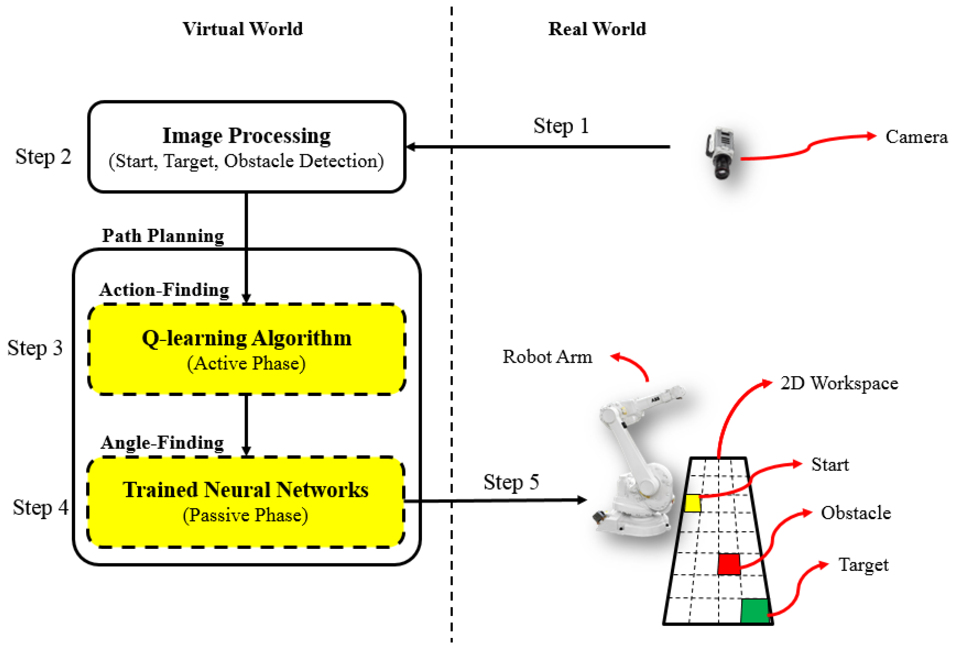
To summarize, the proposed method includes following five steps:
Capturing a picture from the top view of the 2D workspace;
KNN image processing to detect start, target, and obstacle cells;
Using the Q-learning algorithm to find the best path from start to target while avoiding collision with the obstacle (Active phase);
Using the trained neural network to find the joints angles of the found actions (Passive phase);
Implementation of the obtained sequence of joints angles on the robot arm in the real world or simulation world.
As it can be seen, in each step of our hybrid method, we try to use the simplest and fastest way because it would result in a fast and simple path planning method overall. In detail, in step 1, we can use a low-resolution image to increase the speed of image analysis because the start, obstacle, and target cells are distinguished by their colors which can be detected even in low-resolution images. In step 2, we use the KNN algorithm because it is one of the simplest classification algorithms which does not need to be trained. In step 3, we use a simple action space to model it in a programming software without needing a linking the simulator with programming software; we additionally use Q-learning because it can help us to find the optimal path. In step 4, instead of using IK and table lookup, we use a trained neural network that is fast. These simple tasks do not interfere with path planning goals. The performance of our hybrid method is evaluated and tested in simulation and real world in the next section.
3. Simulation and Experiment Results
In this section, the method described in the previous section is implemented in the simulation world and experimental setup. Then, their results are presented and discussed.
3.1. Simulation Results
Robot simulation is an essential tool in every robot researcher’s toolbox. A well-designed simulator makes it possible to test algorithms, design robots rapidly, and perform regression testing using realistic scenarios. Many simulators can be used in the simulation. RoboDk, Webots, Gazebo, SimSpark, Roboguide, MotoSim, RobotExpert, RobotStudio, and RobotSim are some of the most important of them. While robot simulation software vary in feature sets and capabilities, they all share a few common things. They are simulation tools built to replicate real-world robotic applications, considering every environmental and physical factor and testing for possible variables.
In this section, to ensure the performance of presented hybrid method, we test it in the RoboDK simulator before implementing it in the experimental setup. This helps to make sure that the technique is safe and the robot does not collide with itself, the obstacle, and its environment.
RoboDK, developed by Albert Nubiola, is an offline programming and simulation software for industrial robots. This simulation software can be used for many manufacturing projects, including milling, welding, pick and place, packaging and labeling, palletizing, painting, and calibration [
16].
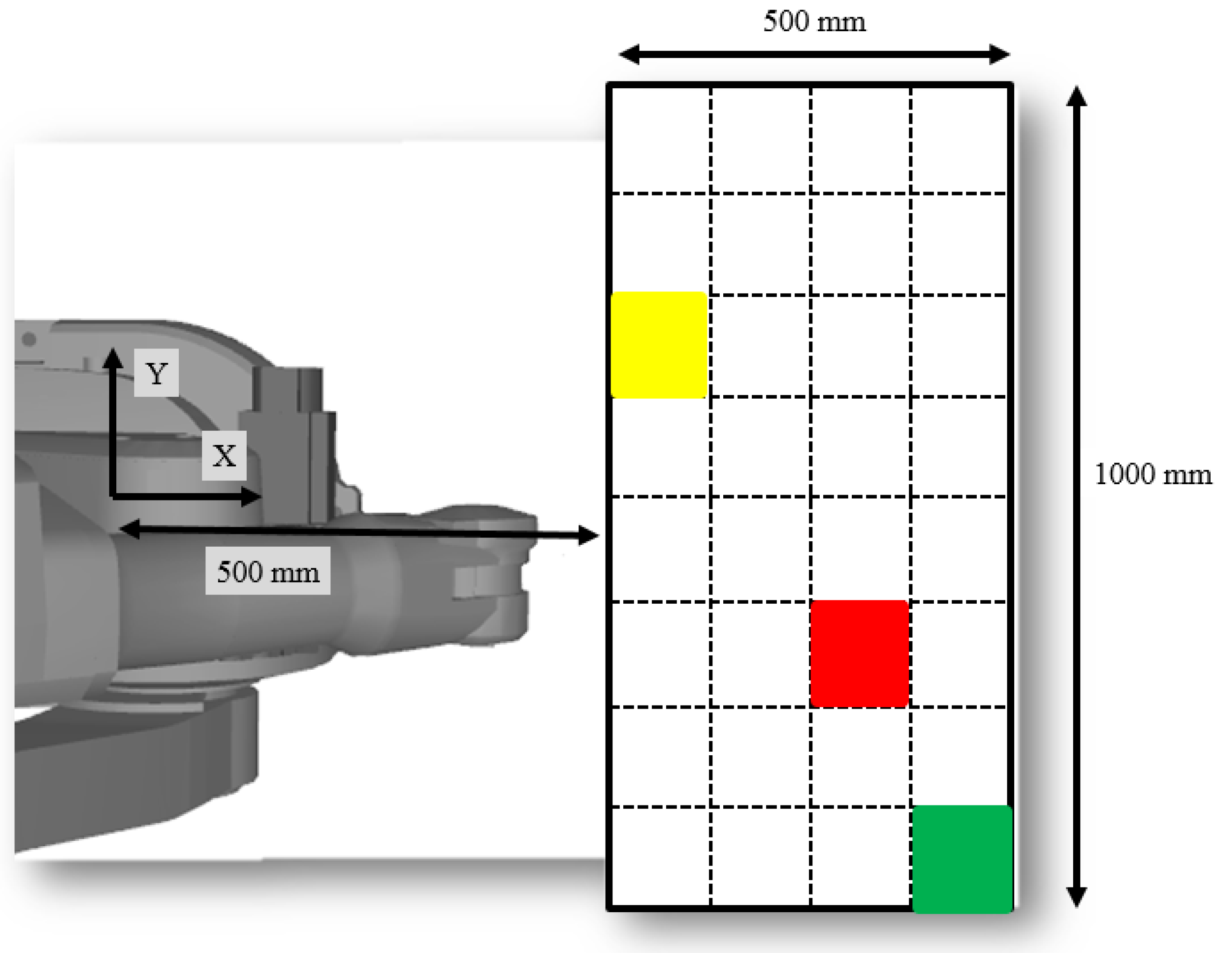
As explain in step 1, we take a photo from the top view of the workspace, as shown in
Figure 4. This includes a rectangular workspace with dimensions of 1000 mm by 500 mm, a yellow square as the start point, a red square as the obstacle, and a green square as the target with dimensions of 125 mm by 125 mm. In step 2, we use the KNN algorithm to find the coordinate of the center of the colorful areas. In this image, given that the reference coordinate system shown in
Figure 4, which is located in the center of the robot arm, the found coordinates of start, obstacle, and target via image processing are (+565,+189), (+801,−193), (+920,−434), respectively.
In step 3, the indexes of the cells of start, obstacle, and target are determined. The indexes of start, obstacle, target cells whose coordinates mentioned in the previous paragraph are (3,1), (6,3), (8,4), respectively. Then, we use them in the Q-learning algorithm to find a sequence of actions from the start cell to the target cell while avoiding collision with the obstacle cell. Inspired by the windy grid world problem, in each cell of the gridded workspace, the best action is obtained so that the agent gets the maximum accumulate reward.
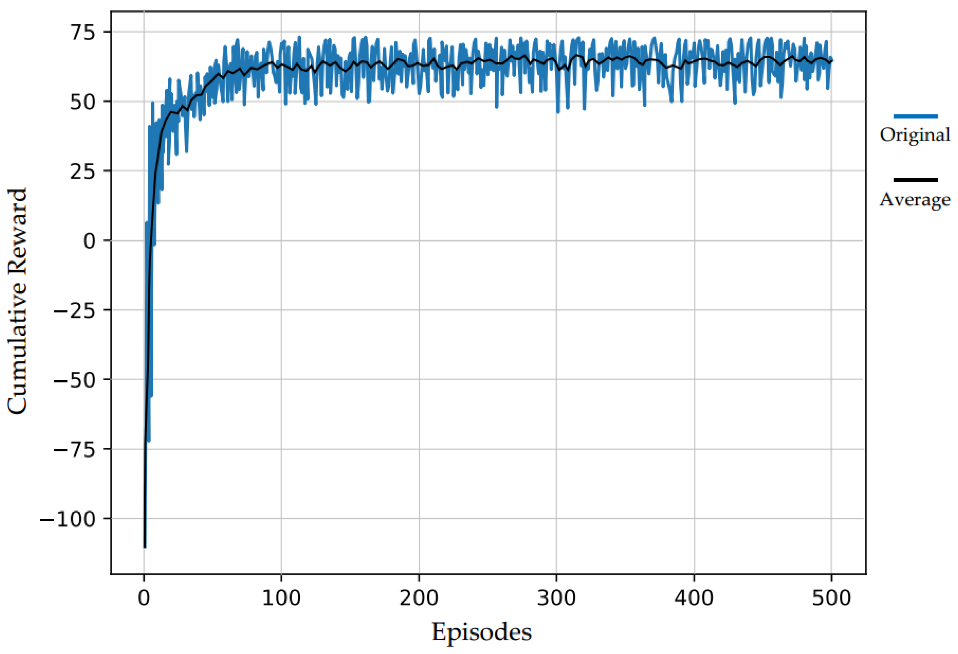
In this article, the values of learning rate (α), discount factor (γ), and probability of exploration (ε) are equal to 0.5, 0.9, and 0.1, respectively. The cumulative reward value is monitored while running the Q-learning algorithm for the environment shown in
Figure 4. Given
Figure 5, we can observe that the cumulative reward converges quickly as the episode increases, which implies the algorithm finds the optimum actions efficiently. It additionally demonstrates that the agent finds actions by the proposed action-finding method such that it not only reaches the given target mostly but also maximizes the return due to the quickly converged reward. Furthermore, since this method uses a simplified state, action, and environment compare with other RL-based path planning methods [
3,
8,
17,
18], it reaches the maximum cumulative reward value in fewer episodes. Consequently, it significantly reduces the required time for path planning.
As
Figure 5 shows, during training, the cumulative reward generally increases until finding a path that leads to the maximum reward and begins fluctuating. This fluctuation happens due to the marginal probability of a non-optimal action being chosen at each step in epsilon-greedy exploration policy, even though an optimal path has been found. In order to better understanding the trend of the cumulative reward and showing concise reward value, the average rewards were added to the diagram.
In
Table 1, the best actions provided by the Q-learning algorithm are shown for the current workspace. By following the sequence of actions from the start cell in yellow, the robot can reach the target cell in green.
Given
Table 1, the end-effector starts from the start cell in (3,1) and moves down to reach cell (4,1). Then, it moves downward four times to reach cells (5,1), (6,1), (7,1), and (8,1). Finally, it moves rightward three times and passes through the cells (8,2) and (8,3) to reach the target cell in cell (8,4). In summary, the obtained actions and passing cells are written as a set of sequence of actions and cells as reported in the following:
| Actions: | {Down, | Down, | Down, | Down, | Down, | Right, | Right, | Right}; |
| Passing cells: | {(3,1), | (4,1), | (5,1), | (6,1), | (7,1), | (8,1), | (8,2), | (8,3), | (8,4)}; |
In order to use actions in the neural network, we rewrite their numerical forms as follows:
| Numerical form of actions: | {2, | 2, | 2, | 2, | 2, | 4, | 4, | 4}; |
Where Up is denoted by 1, Down is denoted by 2, Left is denoted by 3, Right is denoted by 4.
With the help of cells’ indexes and actions obtained in the previous step, in step 4, a neural network that was trained by the data set is used to determine the joints angles. As mentioned, the number of neural network inputs is three, including row index of the cell (i), column index of the cell (j), and action. Thus, according to the obtained data, the neural network inputs are as follows:
| Input of neural network: | {[3,1,2], | [4,1,2], | [5,1,2], | [6,1,2], | [7,1,2], | [8,1,4], | [8,2,4], | [8,3,4]}; |
Where are written in the form of [I-index, J-index, Numerical form of Action].
The outputs should be the required angles to move from the cell (3,1) to down, move from the cell (4,1) to down, move from the cell (5,1) to down, move from the cell (6,1) to down, move from the cell (7,1) to down, move from the cell (8,1) to the right, move from the cell (8,2) to the right, and move from the cell (8,3) to the right, respectively. The angles of the start cell are determined as [18°, 47°, 49°, 1°, −6°, 198°]. The joints angles of found actions via the trained neural network are as follows:
| Angles: | | |
| {[18°, 47°, 49°, 0°, −6°, 198°], | [6°, 47°, 51°, 0°, −8°, 186°], | [−7°, 46°, 51°, 0°, −8°, 171°], |
| [−20°, 46°, 49°, 0°, −6°, 158°], | [−29°, 46°, 43°, 0°, −1°, 149°], | [−34°, 46°, 38°, 0°, 3°, 144°], |
| [−32°, 47°, 28°, 0°, 12°, 146°], | [−28°, 51°, 13°, 0°, 23°, 150°], | [−25°, 54°, 4°, 0°, 29°, 153°]}; |
All findings in active and passive phases are summarized in
Table 2.
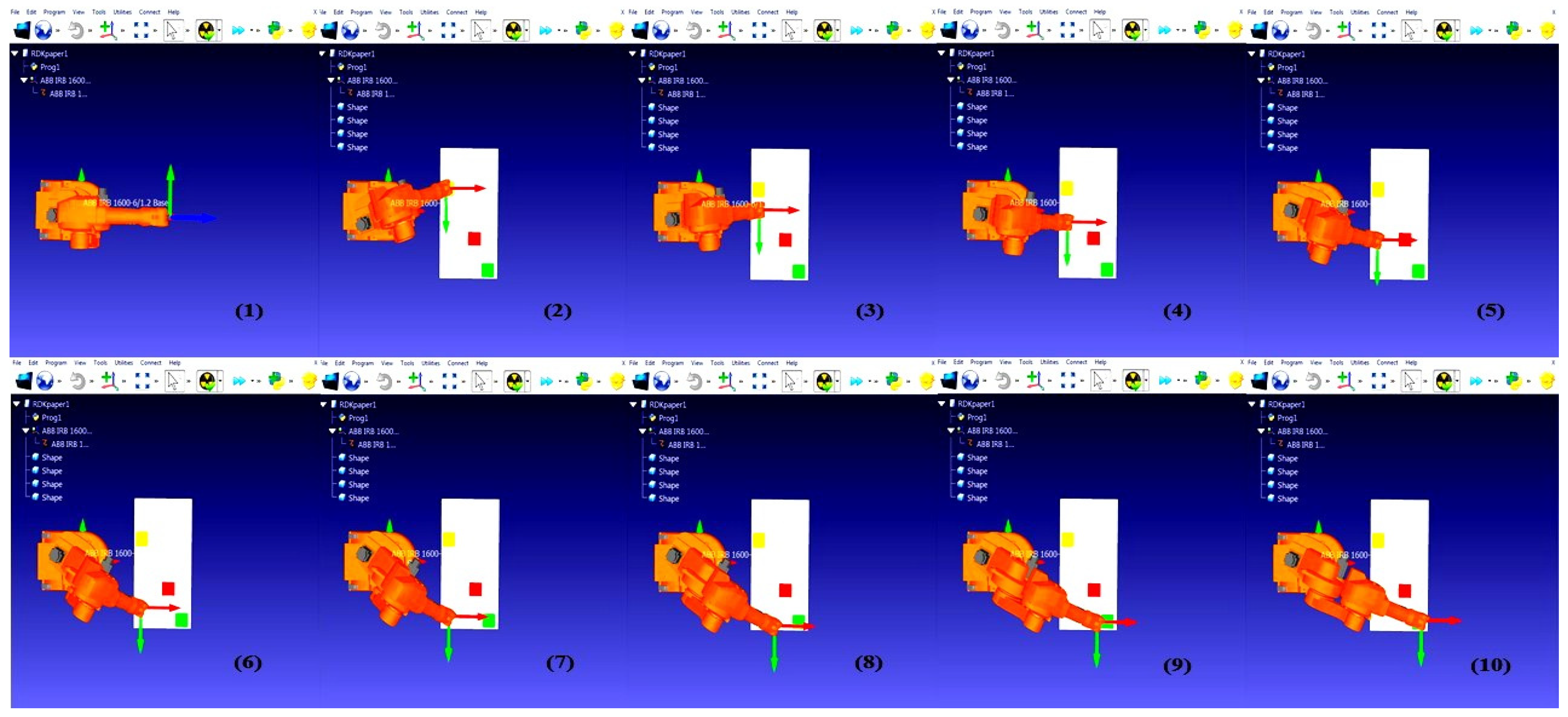
The simulation of our hybrid method helps us to evaluate its performance and safety before implementing it on a real-world experimental setup. Therefore, we can identify joints angles implemented in the RoboDK simulator step by step from the start cell to the target cell, respectively.
Figure 6 shows this process.
3.2. Experiment Results
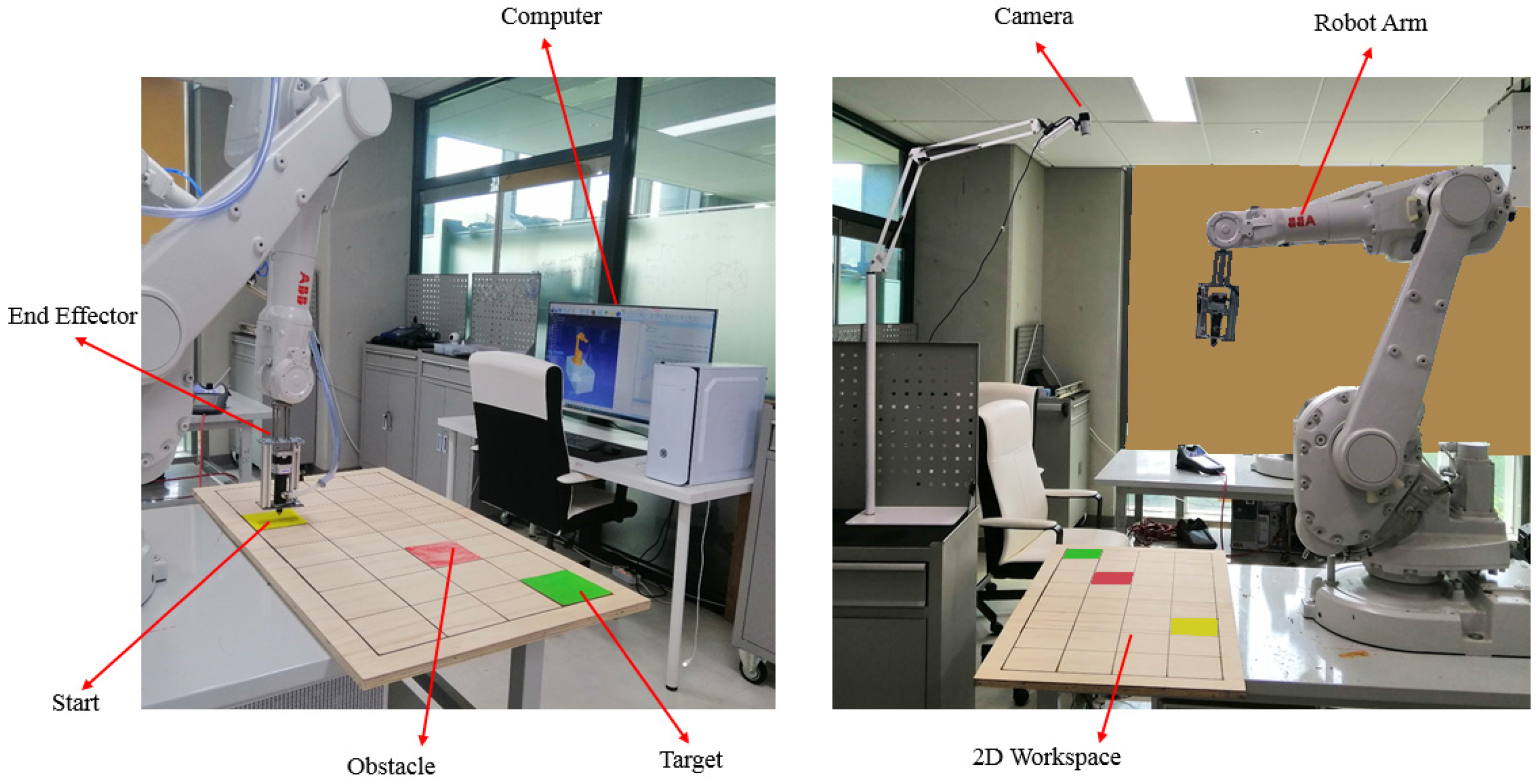
After implementing the hybrid method in the simulation world and confirming the safety during its operation, we can implement it using a real robot arm. In this regard, the experimental setup is presented at first.
Figure 7 shows the setup used to test the presented method. In this setup, a camera installed at the top of the workspace covers this area. Moreover, the robot arm is fixed on the next left side of the gridded workspace, just like the construction robot in a factory near a conveyor belt in a production line. Additionally, a computer is connected to both the camera and robot arm. All the algorithms that exist in this method, including the KNN algorithm (Image Processing), Q-learning algorithm (RL), and neural network, are performed by the computer.
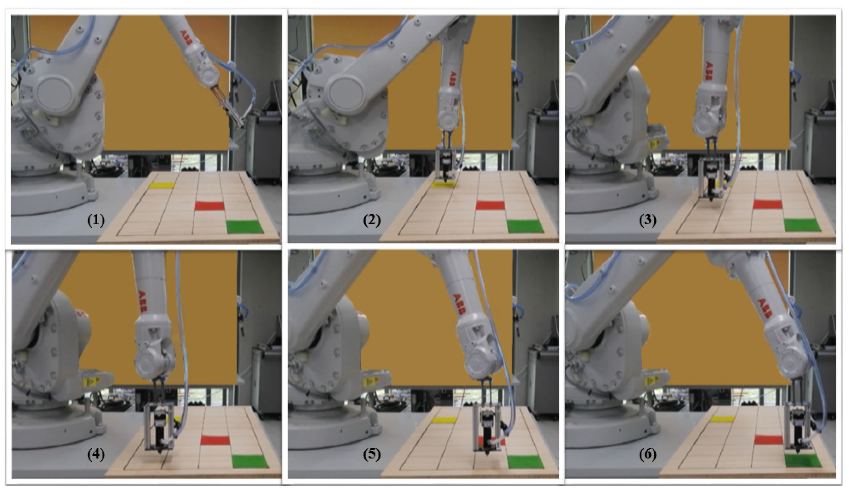
Like the previous section, the image is processed in this part, then the start cell, obstacle cell, and target cell are obtained. Next, using the Q-learning algorithm, the actions are determined. After that, the joints angles are obtained by using the trained neural network. Finally, the found joints angles are implemented in the real robot.
Figure 8 shows the real-world test process. As shown in the images, the end-effector moves from the start cell and follows the path; eventually, it reaches the target while avoiding the obstacle.
Taking the simulation and real-world test results into account, we prove that the proposed hybrid method is a unique path planning approach that has several advantages and resolves the shortcomings of previous path planning methods. This hybrid method has two different active and passive phases to reduce complexity and improve slowness. Unlike the previous methods, which directly tried to find joints angles, this hybrid method first uses simple cells and actions to find optimal actions. Second, this method uses a trained neural network to obtain required joints angles concerning the actions in each cell of the path found in the active phase. The combination of these two active and passive phases is the new approach proposed in this article, which significantly increases the speed of robots in a production line and improves the complexity of path planning. As a result, it reduces computational costs and increases the speed of manufacturing, which causes factories to take advantage economically and perform efficiently.
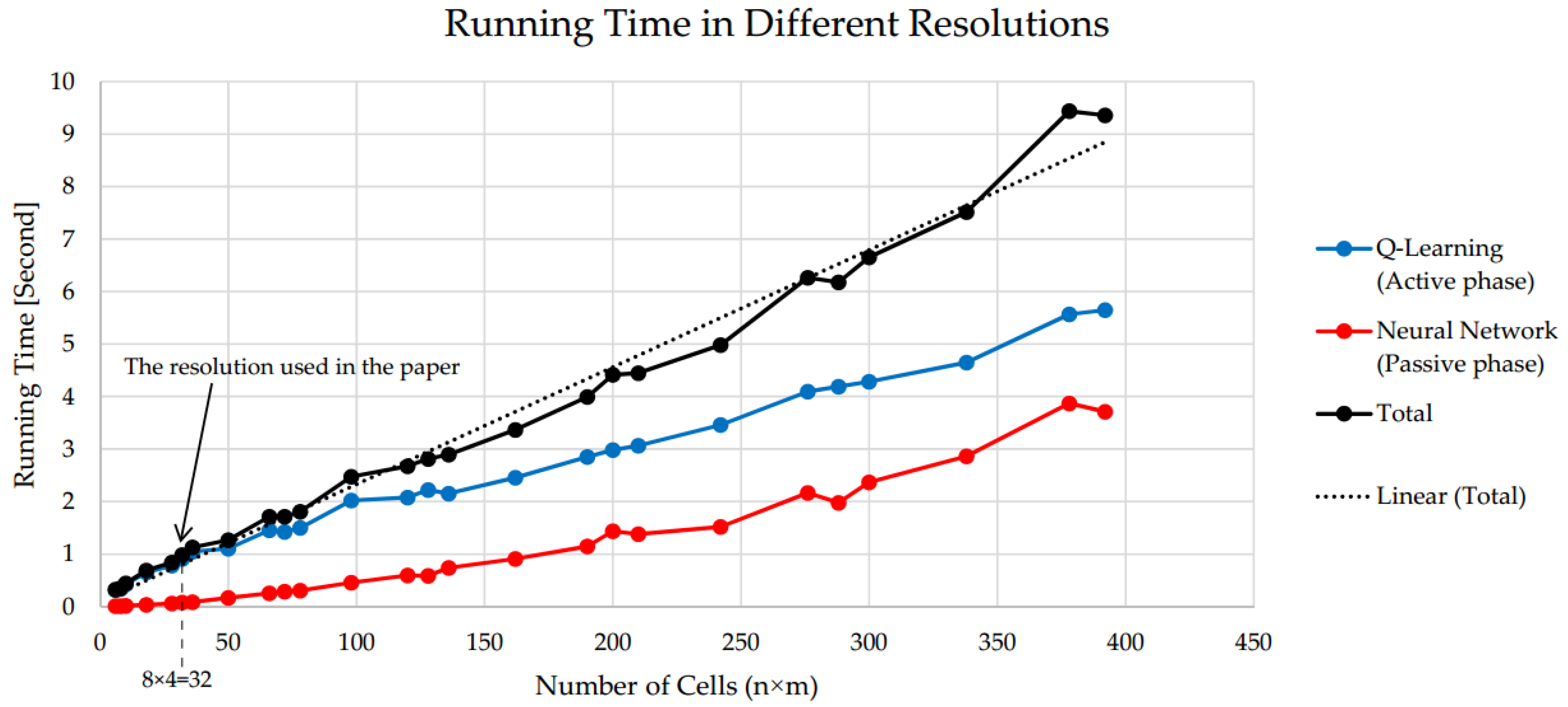
To understand the speed of the proposed hybrid method,
Figure 9 shows the running time of codes, including active phase (Q-Learning) and passive phase (Neural Network), as well as total running time, which is actually the sum of them. These times have been plotted in different numbers of cells of the gridded 2D workspace (i.e., different resolutions). As we highlight in the previous section the neural network completed its training, and here is the time of using trained weights in the joint angles finding phase. As
Figure 9 shows, the running time of Q-learning code is generally longer than that of neural network code because a learning algorithm requires to interact with the environment modeled in programming software to learn optimal actions, but the neural network does not. Therefore, we call them as active and passive phases, respectively. As shown in the below plot, since the resolution in our experiment is eight by four, we have thirty-two cells, so the total running time of this hybrid method for that particular resolution is around 1 s.
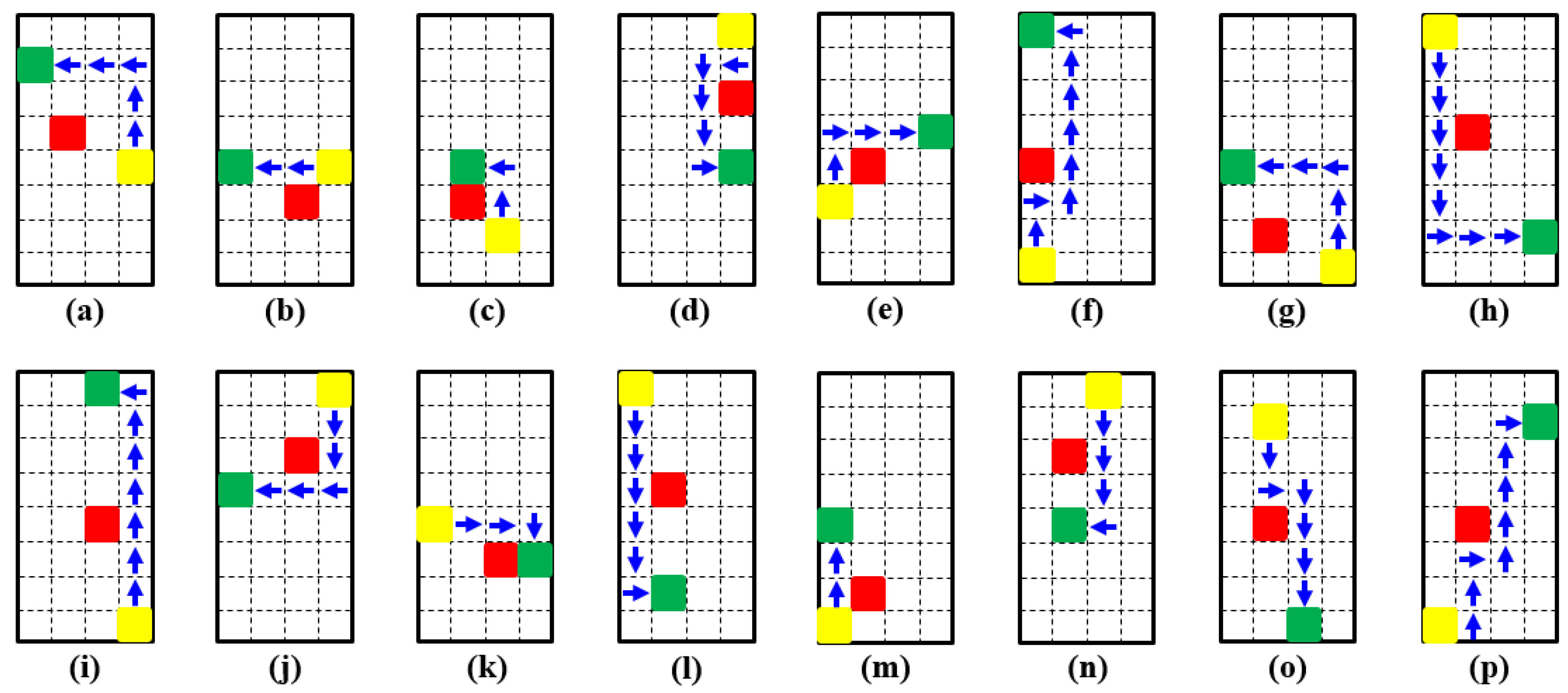
To evaluate the performance of the method in different situations, we test it in various configurations. The start, obstacle, and target cells are placed in different cells arbitrarily. An attempt has been made to cover all different types of configurations. Those configurations are presented in
Figure 10.
The running time of these different configurations are obtained and are presented in
Table 3. It is obvious that when the start and target cells are close to each other, the running time is slightly less than when they are far apart. This is because, since they are close to each other, during the exploring for the target cell, the path is found in fewer episodes. Additionally, since the number of actions is small due to the short path, fewer joint angles are calculated by the trained neural network. Therefore, the total running time of the code is reduced.
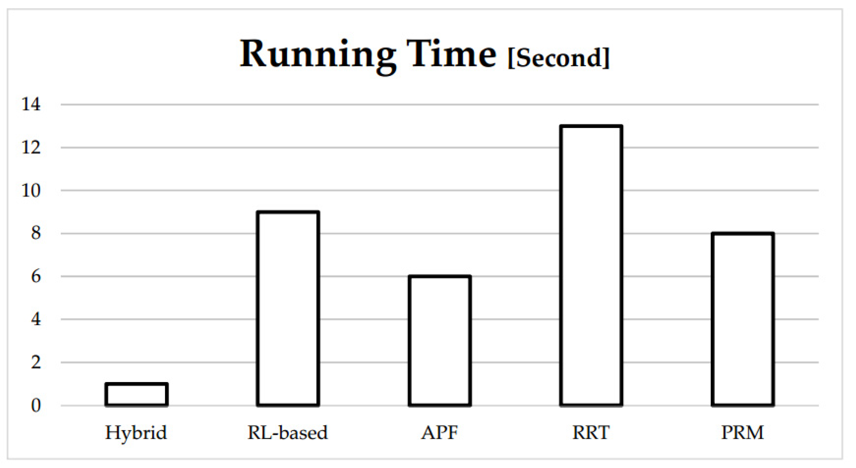
In order to compare the speed of our hybrid method with conventional path planning methods such as RL-based, APF, PRM, and RRT, we run a simple code of each method on the same computer to compute its running time. It is worth mentioning that we downloaded Atsushi Sakai’s APF and PRM (2020), Fanjin Zeng’s RRT (2019), and Valentyn N Sichkar’s RL-based (2018) from Github [
19,
20,
21]. Then, according to our subject, we change and modify their codes and make them similar to our work to become comparable with ours. As can be seen in
Figure 11, our hybrid method needs less running time to do the path planning process under the same conditions, which means it is faster than traditional methods due to using separate active and passive approaches. In fact, our hybrid method makes finding the path faster and simpler in two ways. First and foremost, in the passive phase, we save time by spending a fraction of time before path planning and using it during path planning. In other words, we spend time training the neural network before path planning and use the trained weights during path planning. This is because, unlike the training mode of a neural network which is time-consuming, the using mode takes less time. Second, in the active phase, instead of linking simulators with programming software to obtain a sequence of joints angles, we use simplified state-action spaces to simulate the agent-environment interaction. These two factors have led our hybrid method to reduce the running time and increase the speed.
Future research could examine the performance of this method in dynamic environments in which obstacles and the target continuously change. In other words, since this hybrid method is fast, it can be used for almost real-time path planning. In addition, future research could expand the 2D workspace to a 3D workspace by providing a 3D gridded world and further actions. Finally, future work can improve the limitations which there exist in the image processing section, such as using different colors.


