1. Introduction
To minimize software testing efforts by predicting defect-prone software modules beforehand, many software defect-prediction (SDP) approaches, as described in [
1,
2,
3,
4,
5,
6,
7,
8], have been presented so far. These studies showed that SDP models analyze software metrics data to predict and fix bugs early in the software-development process to improve software testability and to therefore improve the overall software quality [
9].
These prediction models perform well (more accurately) if the software metrics data analyzed are stable. However, the prediction performance of these models may degrade if metrics data evolve dynamically over time. This change is affected by the variation in the underlying properties of the metrics data. This variation in the properties of the data over time is known as concept drift (CD) [
10]. One of the causes of these changes might be the change in hidden variables of data that cannot be measured directly [
11].
SDP aims to ease the allocation of constricted Software Quality Assurance (SQA) resources optimally via prior prognosis of the defect-proneness of software components [
9]. The degradation in performance of prediction due to the presence of CD may significantly affect the detection of bugs in the software, thereby putting a negative impact on software-testing efforts and causing an increase in the software-development cost. As a result, the quality of the software, which is an important factor in the software-development life cycle process, can degrade. Therefore, one solution of this problem is to first detect drift in the currently processed data and to therefore handle the detected drift before further prediction.
Only a couple of studies [
10,
12,
13,
14] have examined CD in SDP. Ekanayeke et al. were the first to investigate the presence of CD in SDP. They proved that software-defect data are prone to CD. The recent work by Kabir et al. [
13] used an existing Drift Detection Method (DDM) [
15] to detect CD and its related impacts on SDP performance. They evaluated the statistical significance of this method using the chi-square test with Yates continuity correction. Bennin et al. [
14] recently assessed the existence of CD and its impact on performance of SDP. These works create the foundation and are the motivational factors for discovering and handling concept drift in software-defect prediction. Therefore, further work is required to better detect CD points and to adapt the detected CD in SDP. To the best of our knowledge, none of them used the paired learner (PL) to discover concept drift in SDP.
In this paper, we present a dynamic approach based on paired learner to detect and adapt to the concept drift in software-defect prediction. Dynamic behavior occurs as the learned experience from the processed modules is used to predict the presence of drift in unseen modules. We investigate the presence of sudden and gradual drifts in software-defect data. The presented approach first divides the validation dataset into assorted separate subsets using a partitioning technique, and then, trains one of the learners using modules in all subsets exercised previously and the other learner from the modules in the recent subset only. Afterwards, both learners are used to disjointedly predict on unseen data modules; then, the difference in predictions of the two learners is compared to a threshold value for the purpose of detecting drift. If drift is detected, the first learner is updated to handle the CD.
The following are the contributions of this study:
We present a dynamic approach based on paired learner to detect and adapt to CD in SDP.
An exhaustive assessment of the presented method for several defect datasets collected from different open source data repositories is presented. We evaluate the presented method in terms of the improvement in detection of concept drift points using the prediction model in SDP.
We present a comparative evaluation of the presented method with the base learning methods used in the study.
In our current study, we aim to answer the following research questions, which were not answered by previous studies:
RQ1—Available studies on CD in SDP are mainly focused on showing the proneness of defect data to concept drift. Therefore, there is a need to explore how significantly the concept drift points in numbers are present in defect data used for SDP.
RQ2—Studies in other domains of data analysis proved that CD adaptation is required to prevent performance degradation of the prediction model. No previous studies in SDP ever used paired learner for CD adaptation in SDP. Therefore, how would the proposed approach adapt to the CD discovered in SDP?
In this work, we provide a procedure for concept-drift detection and adaptation in SDP along with a comparative analysis of the number of drift points discovered to answer question 1. In order to answer question 2, we provide an algorithmic procedure to explain the CD adaptation procedure and a comprehensive comparative performance analysis of the results as proof by implementing the window-based approach.
The remainder of this paper is organized into the following sections. The background of the study is presented in
Section 2.
Section 3 presents the synopsis of the related studies. A detailed description of the proposed approach is presented in
Section 4. The experimental settings are presented in
Section 5.
Section 6 presents the experimentation results and discussion. The comparative analysis results are provided in
Section 7.
Section 8 describes the threats to validity. Finally,
Section 9 concludes the paper.
2. Background
2.1. Definition of Concept Drift
Concept drift has been previously studied by many researchers in different domains. The authors in [
16,
17] provided a formal definition of concept drift in terms of the statistical properties of a target variable over a period of time and the joint probabilities of the feature vector and target variable. These researchers discovered three sources of CD in terms of the joint probabilities of a feature vector and a class variable. Using these relations between probabilities, the authors characterized two types of drifts i.e., virtual and real. In terms of statistical properties of target variable, we can define CD as follows—
If represents the statistical properties of target variable at time t and represents the statistical properties of target variable at time t + 1, then there is CD if ! = .
2.2. Concept-Drift Types
The change in concept over a period of time is known as concept drift. This concept change may happen in four ways, giving four types of CD categories, defined as follows:
There is a concept change within a short duration of time (Sudden).
An old concept is gradually replaced by a new concept over a period of time (Gradual).
A new concept is incrementally reached over a period of time (Incremental).
The old concept reoccurs after some time (Reoccurring).
2.3. Concept-Drift Handling
Dong et al. in [
18] proved and showed that a well-trained defect-prediction model may output inaccurate results if the data distribution changes over time. They also proved that training a prediction model becomes more difficult in such scenarios. This points out that concept drift must be handled if data distributions change over time. In our current study, we present an approach to detect and handle concept drift in SDP.
While predicting defects in software, drift could happen when the trained predictor does not perform well due to the presence of a changing concept. Therefore, these changing concepts must be discovered to update the predictor. Our proposed approach, as described in the following sections, efficiently discovers the concept-drift points in software-defect data.
3. Related Work
A few investigations revealing assessments of CD in SDP are found in the literature. Below, we talk about these works, which are summarized in
Table 1.
Rathore et al. [
8] evaluated various fault-prediction research studies from 1993 onwards. They classified the revision of these studies into three groups: data-quality issues, fault-prediction techniques, and software metrices. They found that most fault-prediction studies experimented eith publicly available, object-oriented and process metrics data. They also found that the performance of fault prediction models vary with datasets used for prediction.
Hall et al. [
7] reviewed the prediction performance of thirty-six defect-prediction techniques published during 2000 to 2010 in software engineering. The major contributions of that study were centered on the classification of techniques on the grounds of a prediction model, software metrics, the dependency of variables, and the prediction performance of SDP. They proved that prediction methods using naive Bayes and linear regression (LR) produced better defect predictions than C4.5 and support vector machine. The prediction results for object-oriented software metrics were found to be better than other LOC or complexity metrics. On the other hand, they did not provide any taxonomical classification of SDP models.
These exhaustive review studies on SDP showed that the SDP models are trained using the historical metrics data. Thereafter, these models use this learned experience to predict the number of faults or the presence/absence of faults in the currently used software modules. This provided the basis for diagnosing the effects of changing data distributions in SDP processes. Only a few studies in this domain have been presented so far, as reviewed below:
Ekanayake et al. [
10,
12] were the first to explore the idea of CD in SDP and provided the basis for predicting the occurrence of CD in these studies and for inspecting and evaluating the causes of CD in prediction performance. The authors in those studies determined that the accuracy of prediction changes when chronological datasets are used for training a prediction model. They attributed the altering outputs to changes in the data characteristics. Using an analysis of the files and the defect-fixing procedure of software programs, the authors noticed that changes made to software files tend to drift the concept in the distribution of data, accordingly affecting the outcome of the defect prediction. They evaluated their model on CVS and bugzilla data from four open-source projects: Mozilla, Eclipse, Open Office, and Netbeans. They discovered that variations in the bug-fixating process and the coders responsible for editing the implementation codes are mainly responsible for changes in the quality of the prediction.
Kabir et al. [
13] used a CD-detection method proposed by Gama et al. to discover CD in defect datasets. They applied the Chi-square statistical test with Yates continuity correction to detect CD. They selected two windows for data analysis, recent and overall, through Naive Bayes (NB) and Decision Tree (DT) classifiers and used the accuracy measure to detect drifting points in the data.
A recent study by Kwabena E. Bennin et al. [
14] investigated the impact of CD in SDP. They used defect datasets from five open-source projects and showed that the performance of prediction models is not stable over time when using historical datasets for training the static predictor. They suggested designing a tool to detect the CD before training.
The research in these studies did not provide any solution for handling concept drift in SDP, and they did not explore paired learner for CD adaptation in SDP. Therefore, in our current work, we provide the solution to overcoming the listed shortcomings. We proposed a dynamic approach for detecting CD in SDP. Thereafter, we perform a comprehensive comparative analysis of the results using the Wilcoxon statistical test.
4. Proposed Approach
In this section, we present the proposed approach to handling CD in software-defect prediction. The concept of paired learner was previously discussed by Bach and Maloof [
19].
4.1. Paired Learner
Bach and Maloof [
19] presented their study on a new CD adaptation method named paired learner. This method consists of two learners (stable and reactive) as a pair, hence the name paired learner. Stable PL learns from all data samples from beginning or from the last drift point onward, while the reactive learner utilizes learning from the data samples from the window in recent time. They used reactive learner to discover drift in the data, whereas the stable learner was used for prediction. The difference in accuracies of these two learners along with a threshold parameter value was used to discover drift in two synthetic and three real-world datasets. Their proposed method analyzes data in online mode processing one example at a time.
Zhang et al. in [
20] presented their study using a long-term stable classifier and a dynamic classifier to detect both sudden and gradual changes. They presented a paired ensemble for online learning for CD and class imbalance.
4.2. Proposed Approach Based on PL
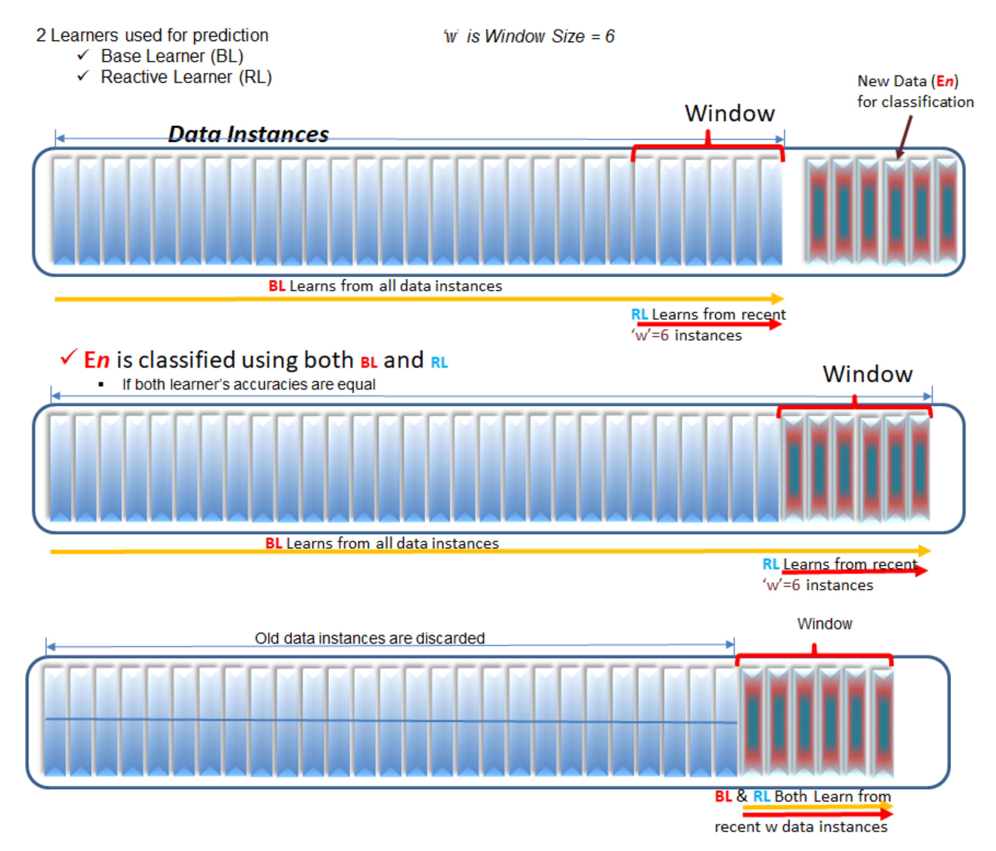
In this section, we present a PL-based approach in which batches of data examples are processed at a time to predict the presence of defects in the batch. The stable learner is trained using past data, whereas the reactive one always learns from the recent window only. Both the stable and reactive learners of the pair predict at the same time using the software metrics data samples in the currently processed window. The difference in accuracies of the learners in the pair is used to detect drift in the data. If drift is detected, then it is assumed that the past learned experience of the stable learner is causing harm as the reactive one performs better. Therefore, it is time to update the stable learner of the pair. As a consequence, the algorithm forces the stable learner to be updated by making a new instance of it and therefore training the newly created stable learner with the data samples in the currently processed window only. This removes the chances of affecting the performance of the paired learner from the learned experience using old data examples.
Figure 1 below depicts the working of the proposed approach. A batch size of six samples from defect data was selected to depict the pictorial representation of the concept. At any point of time, the stable learner (SL) of the pair is trained using all examples from the beginning or last drift points onward and the reactive learner (RL) is trained using the examples in recent batch. As soon as a new batch of examples arrives, both SL and RL make predictions based on their training until then, as described earlier. The approach uses actual values of a target variable to compute the performances of SL and RL in terms of correct classifications and misclassifications. As RL and SL predict on the same test data, the difference in their performances is used to detect drift. If CD is detected, the approach forces the SL of the pair to be reinitialized by the current learning experience of the RL. Then, both SL and RL are trained using the examples in the currently tested batch and RL is made to forget its learning from the previous batch. Therefore, at any point of time, RL’s learning experience is only from the examples in the recent window.
Algorithm 1 presents the algorithmic procedure of the proposed approach. The input to the algorithm (line 1) is a collection of example instances from the defect dataset, window size (k) (line 4), threshold value () (line 5) and the learners (S, R) (line 6,7). Both stable and reactive learners of the pair are initially trained (line 12) with the data samples in the first window. A loop (line 13) repeats the execution until all samples in the dataset are evaluated. The stable learner predicts (line 14), whereas the reactive one performs prediction (line 15) using the data samples in the currently processing window. The number of places in the current window where predictions of the reactive learner are correct whereas that of the stable learner are incorrect are computed (lines 16–20). This count is then compared with the user-supplied threshold value for detecting drift. If drift is detected (line 21), it is handled by updating the stable learner (line 23). Finally, the training experiences of both the learners are enhanced by the data examples in the currently exercised window (lines 27–28) before the next iteration proceeds.
The workings of the algorithm are described in
Figure A1. This diagram represents the block diagram showing various steps followed in the proposed approach.
| Algorithm 1 PL-based approach for CD detection and adaptation in SDP. |
|
▹ Inputs to the Algorithm
|
|
1: Input: D = : n is the size of defect dataset
|
|
2: : vector of independent variables
|
|
3: : The value of dependent variable
|
|
4: k: size of the window
|
|
5: threshold for drift detection
|
|
6: S: stable learner
|
|
7: R: reactive learner
|
|
8: : k predicted values by stable learner
|
|
9: : k predicted values by reactive learner
|
|
10: C: count to hold miss-classifications, initially 0
|
|
11: index: start counter for stable, initially 1
|
|
▹ Initially Train the models using samples in the first window
|
|
12: S.train(, ), R.train(, )
|
|
13: for to do |
|
▹ Make Classification using stable learner
|
|
14: |
|
▹ Make Classification using reactive learner
|
|
15: |
|
▹ Count misclassifications
|
|
16: for to k do |
|
17: if and then |
|
18: |
|
19: end if |
|
20: end for |
|
▹ Detecting CD in current batch of data samples
|
|
21: if then |
|
22: Output concept drift at i and adapt to drift
|
|
▹ New instance of SL
|
|
23: |
|
24: index = i |
|
25: end if |
|
26: C = 0
|
|
▹ Train the learners with corresponding set of data
|
|
27: |
|
28: |
|
29: end for |
5. Experimental Settings
The study by Žliobaitė et al. [
21] showed that machine learning models can be applied in software engineering. The study by Lin et al. [
22] presented a three-stage process (Learning⟶Detection⟶Adaptation) for handling CD. In our presented study, we chose to use machine learning models for finding and adapting to concept drift while predicting defects in software-defect datasets.
5.1. Choosing the Base Learners
For our experimentation, we used paired learners of naive Bayes (NB) and random forest (RF) classifiers (also known as PL-NB and PL-RF). We chose these learners due to the following reasons:
Naive Bayes has been widely used in the literature [
13,
19,
23]. NB stores the distributions for every class and for every attribute given the class. It also stores the frequency counts of each value for symbolic attributes and the sum of the values along with sum of the squared values for numeric attributes. These distributions are estimated from the training data. NB computes the prior and conditional probabilities for each class, assuming that the attributes are conditionally independent. Afterwards, it uses the Bayes theorem to predict the most probable class as follows:
Let the prior probability for each class be .
The conditional probability for each class is ; here, is the instance j.
Then, the most probable class H is . These steps, involve adding and subtracting counts and values to/from the appropriate distributions, are easy and efficient to implement for NB.
Previous studies [
1,
2] showed that RF outperformed other classification techniques. The random forest classifier consists of many decision trees operating as an ensemble. Each tree in the random forest makes a class prediction, and the class with the majority of votes becomes the model’s prediction. The probability of making correct predictions increases as the number of uncorrelated trees are increased in the RF model. Random forest is an efficient algorithm for large datasets. It generates an internal unbiased estimate of the generalization error as the building of forests progresses.
We also evaluated a few available learners including decision tree (DT), K-nearest neighbor (KNN), naive Bayes (NB), random forest (RF), and support vector machine (SVM) used in the defect-prediction literature. While predicting the defects in a software dataset, the accuracy scores reported by these learners are used to select two top-performing classifiers (NB and RF) for our experimental study.
5.2. Choosing the Dataset
We chose the versions of publicly available NASA (JM1 and KC1) and Jureczko PROP datasets because they have already been used in past research [
1,
3,
13,
24,
25,
26,
27,
28,
29] on CD and the Jureczko datasets has been better explained by Jureczko in [
30]. We ran the proposed methods PL-NB and PL-RF on these selected defect datasets one by one and computed their performance measures (accuracy and area under the ROC curve). We summarized the experimentation results in both tabular and graphical representations for better understanding.
Summary of Datasets
We conducted our experiments on the datasets collected from the PROMISE and SEACraft online public repositories. The JM1 and KC1 datasets consist of Lines of Code, McCabe’s [
31], and Halstead metrics [
32] attribute data, whereas the prop dataset consists of C & K object-oriented metrics [
33] attribute data. The McCabe and Halstead metrics represent the measurements of complexity of the code modules in different forms, whereas the Lines of Code metrics are what the name suggest. McCabe in [
31] presented a metric set that measures the code module’s complexity by computing the possible paths in the program. Furthermore, it used cyclomatic complexity as the main metric in this category and demonstrated that, as the number of branches (paths) in the program increases, the cyclomatic complexity also increases. McCabe focused his intention to deliver a measuring metric that could tell the developers that their software code is over complicated and should be segmented into smaller modules. McCabe suggested to further break-up the software module if its cyclomatic complexity exceeds ten. These metrics were later used for defect prediction in software modules with the reason that modules with higher complexity more probably carry defects. On the other hand, Halstead metrics originated in [
32] and are based on the readability and operations (operators and operands) complexities of the modules. These measurements are used in defect prediction with the notion that, if a program module is hard to read, it will be more likely to carry defects. Eventually, LOC metrics along with the number of comments are used to predict defects in software with the idea that longer modules are more likely to carry defects.
The Chidamber & Kemerer object-oriented metrics suite originated in [
33] and consists of six metrics (WMC, DIT, NOC, CBO, RFC, and LCOM1) computed for each class. The weighted method count (WMC) is simply a number representing the count for methods of a class and is a measure of how much effort and time is required to develop the class. Researchers later found that a high value of WMC leads to more defects. The depth of inheritance tree (DIT) represents the maximum inheritance path from the derived class up to the root class. Deep inheritance trees stipulate more design complexity. A recommended DIT value is five or less. A high value of DIT has been found to add more defects [
33]. Number of Children (NOC) represents the count for immediate child classes derived from the base. NOC is a measure of the breadth of the class hierarchy. Possibly due to reuse, a high value of NOC has been found to indicate less defects [
33]. Coupling between objects (CBO) represents the number of classes to which a class is coupled. A high value of CBO is not considered good in programming and has been found to indicate defect proneness [
33]. Response for a class (RFC) represents the number of methods in a response set of a class, which is the set of methods that is executed in response to a message received by an object of that class. A large value of RFC indicates that the class is more complex and harder to understand and has been found to indicate more defects. A high value of the lack of cohesion of methods (LCOM) metric also indicates more defects.
Catal and others in [
2] categorized the metrics used in software-defect prediction into six groups: quantitative value-level metrics, process-level metrics, component-level metrics, file-level metrics, class-level metrics, and method-level metrics. The McCabe and Halstead metrics used in this study correspond to the method-level metrics group, whereas C & K object-oriented metrics correspond to the class-level metrics group. The study in [
2] reported that the WMC, CBO (coupling between object), RFC (response for a class), LCOM (lacks of cohesion of methods), and LOC (lines of code) metrics are very useful in predicting defect-proneness in software modules. A more detailed description of the metrics can be found in [
32].
Table 2 and
Table 3 present the summary of the attributes used in the selected datasets for our experiment.
Table 4 represents the summary selected datasets for our experiment. There are 22 attribute features in the NASA datasets and 21 attribute features in the Jureczko datasets. The last attribute in these datasets is the target feature.
5.3. Choosing the Window
Previous studies [
13,
16,
17] on CD have proven that the selection of an appropriate window size is a challenging task because, in scenarios, a small window size may accurately reflect the current data distribution and may identify sudden concept changes more accurately, but it worsens the performance of the system in stable periods. In contrast, a large window improves the performance of the system in stable periods, but its reaction is slow in changing concepts. The training window size can be fixed or variable.
We selected the best fixed, small window based on the ROC-AUC scores and accuracy of prediction for each dataset after repeatedly experimenting with the procedure for different values of the window sizes starting from 100 to 500 samples; refer
Table 5. We were successful in detecting the sudden drift in the experimented software defect data.
5.4. Performance Evaluation Measures
AUC-ROC: We used the area under the ROC curve to compare the performance of the proposed approach. The accuracies of the PL-NB and PL-RF are computed based on the true and false positive and negative values of prediction. Additionally, the number of misclassifications by the stable learner in the window where the corresponding reactive learner made correct classifications along with a user specified threshold value is used to detect CD. Accuracy alone is not used for drift detection to avoid mis-detection in scenarios where the stable learner’s predictions are correct and reactive learner’s predictions are wrong for the first half of the window whereas the reactive learner’s predictions are correct and stable learner’s predictions are wrong for the next half of the window. In such a scenario, as the reactive learner’s accuracy increases and the stable learner’s accuracy decreases because of a changing concept, the accuracies of both the stable learner and the reactive learner are 50%. Hence, the accuracy measure could not detect the changing concept in such a situation. To avoid such misclassifications, the second proposed measure, i.e., the difference in misclassifications of two learners, is used to detect CD.
The area under the ROC curve corresponds to the confidence in positive classifications. As none of the true positive and false positive rates consider the number of true negatives, the classifier performance is not impacted by the skewed class distribution. Therefore, we chose to use these rates to evaluate the performance of the classification in spite of the accuracy measure, which was the same method employed by Lessmann et al. in [
1].
Cost–Benefit Analysis: To determine the cost-effectiveness of SDP models, a cost–benefit analysis of the employed CD detection and adaptation technique is undertaken. In the context of SDP, Wagner first developed the concept of a cost–benefit analysis [
34]. In another real-time application for IoT devices, Anjos et al. [
35] proposed a dynamic cost model to minimize the energy consumption and task execution time to meet the restricted QoS requirements and battery limitations. Using the outputs of SDP models in conjunction with the software-testing process in the software development life cycle, this analysis estimates the amount of testing effort and cost that may be saved. To estimate the defect removal cost of a certain defect prediction model, the analysis model considers the defect removal cost and the defect identification efficiency of different testing phases generated from case studies of different software organizations. Kumar et al. [
36] looked into how a cost–benefit analysis could be used in SDP. We used the model offered in our study to assess the cost-effectiveness of the CD-detection and -adaptation approach.
When defect-prediction results are combined with the software-testing process, Equation (
1) provides the estimated defect-elimination cost (Ec). The Ec value is computed on the basis of the base model results. After executing the proposed CD-detection and -adaptation approach, another E’c value is computed using the same equation. The normalized defect-removal cost after the application of the CD-adaptation approach and its interpretation is shown in Equation (
2). The phenomenon of normalization has been previously presented by Silva et al. [
37] for the computation of normalized RMSE in execution of the hybrid control method for exoskeletons.
when:
The definitions of the notations used are the same as those specified in one of the studies by [
36]:
“Ec: Estimated software defect elimination costs based on software defect prediction results
NormCost: Normalized defect removal cost of the software when software defect prediction along with CD handling is used
Initial setup cost for using software defect-prediction model ( = 0)
Normalized defect removal cost in unit testing
Normalized defect removal cost in system testing
Normalized defect removal cost in field testing
Normalized defect removal cost in integration testing
FP: False positives in numbers
FN: False negatives in numbers
TP: True positives in numbers
Defect identification efficiency of unit testing
Defect identification efficiency of system testing
Defect identification efficiency of integration testing”
The defect identification efficiency of various testing phases is defined as staff hour per defect and is based on research by Jone [
38]. In our study, we used the median of Jone’s defect identification efficiency estimates taken as
= 0.25,
= 0.5, and
= 0.45. The normalized defect-removal cost is derived from Wagner’s work [
39,
40] and is defined as a staff hour per defect. We used the median of these data values in our study.
= 27.6,
= 6.2,
= 2.5, and
= 4.55 are the values used. The study [
36] goes into great detail about the cost–benefit analysis model that was used.
5.5. Statistical Test
Wilcoxon statistical test [
41] is adopted to discover the statistically significant difference between the performances of the two classifiers over time. This test determines whether two or more sets of pairings are statistically significantly different from one another. This test is based on the assumption of independence, which means that the paired observations are picked at random and separately. In our analysis, the two sets of values for the class variable are determined independently by two different learners. Therefore, Wilcoxon signed rank test is suitable to discover the statistical significant difference between the compared sets of values.
To test the hypothesis, Wilcoxon signed rank test is executed with the zero_method, alternative, correction, and mode parameters in default settings. A significance level of 0.05 with a confidence interval of 95% is chosen. That is, for all of the experiments, the null hypothesis is that there is no significant difference between the two data distributions where the observed significance level is greater than or equal to 0.05. Otherwise, the null hypothesis is rejected and the alternate hypothesis is assumed, declaring the detection of concept drift.
The null hypothesis and the alternate hypothesis for the Wilcoxon statistical test may be stated as follows:
Null Hypothesis : There is no difference between the distributions of the two populations.
Alternate Hypothesis : There is significant difference between the distributions of the two populations.
The p-values less than alpha (0.05) indicate that the Wilcoxon test rejects the null hypothesis and accepts the alternate hypothesis.
5.6. Experimental Procedure
This experimentation describes the presence of CD in software-defect datasets. It also reports the improvements in prediction performance as part of handling the discovered CD. Around 9600 sample instances from the NASA jm1 dataset, 2100 from the NASA KC1 dataset, and 27,750 from the Jureczko prop dataset are used for our experimentation. For the jm1 and prop datasets, initially 500 samples are used to train the model. Thereafter, samples in chunks of 500 are used to detect and handle CD in subsequent runs. For the KC1 dataset, chunks of 100 sample instances are used for the experiment following a similar process. We trained the model by taking all of the samples in one window and the only recently used chunk in another window. We iterated this process until all data samples were experimented upon. We used paired learners of naive Bayes and random forest classifiers for the prediction. A threshold value of 95% confidence interval along with the predictions by stable and reactive learners of the pair was used to detect the change in concept.
Initially, we executed the base versions of the NB and RF classifiers to compute the accuracy and ROC-AUC scores.
Secondly, we executed the paired versions of NB and RF to find the concept-drift points.
Finally, we updated the stable learner of the pair to adapt the detected concept drift and computed the accuracy and ROC-AUC scores using the paired versions.
6. Experimentation Results and Discussion
This experiment first found out the presence of CD in our studied software defect datasets using the proposed PL based method. Afterwards, we handled the discovered drift by updating the prediction model. The error rate between the predictions by stable and reactive learners of every experimental run was monitored to investigate the existence of drift.
Table 6 presents the accuracy and ROC-AUC scores obtained after experimenting the PL based method for the jm1, KC1, and 9 versions of the prop datasets.
We monitored the error rate between the classifications using the stable learner on the overall distributions and using the reactive learner on the recent distribution to monitor the changes in recent data distribution. The significant change in error rate between the two distributions indicate the change in concept.
Changes in concept were detected in the experimented prop and jm1 & KC1 defect datasets, discovering drift. Then, the prediction models were updated and obtained better prediction performances, as shown in
Table 6.
6.1. Experimentation on NASA Defect Datasets
This section presents the results obtained after conducting experiments on the NASA jm1 and KC1 defect datasets collected from the PROMISE online public data repository. There are 22 features in the dataset, of which 21 are used to represent feature vectors and 22 are used as class variables. A window size of 500 samples for jm1 and 100 samples for the KC1 dataset was used for the experiment.
The AUC-ROC curves, as shown in
Figure 2a,b, showed that the ROC-AUC scores of PL-NB and PL-RF are better than the ROC-AUC scores of base NB and base RF (Refer
Table 6), respectively. That is to say, the application of PL for CD adaptation in SDP showed significant improvement in the performance of the prediction model.
6.2. Experimentation on Jureczko Prop Defect Datasets
In this section, we presented the results obtained after conducting experiments on versions of the Jureczko ’prop’ dataset collected from the SEACraft [
8] online public repository. There are 21 features in the dataset, of which 20 are used to represent feature vectors and 21 are used as class variables.
The AUC-ROC curves, as shown in
Figure 2a,b and
Figure 3a–i, showed that the ROC-AUC scores of PL-NB and PL-RF are better than the ROC-AUC scores of base NB and base RF (Refer
Table 6), respectively. That is to say, the application of PL for CD adaptation in SDP showed significant improvement in the performance of the prediction model.
6.3. Cost–Benefit Analysis for Realistic Applications of the Proposed Approach
SQA is a process that runs concurrently with software development. It aims to improve the software-development process so that issues can be avoided before they become a big problem. SQA is a form of umbrella operation that covers the entire software-development process. Testing is the process of using every function of a product in order to ensure that it meets quality-control requirements. This might include putting the product to use, stress testing it, or checking to see if the actual service results match the predicted ones. This method detects any flaws before a product or service goes live [
40].
Programming testing is a fundamental activity, and it is over-the-top expensive to test the software defects altogether. An investigation on the Cost of Software Quality (CoSQ) model announced that the expense of software defects in the USA is 2.84 trillion dollars and, furthermore, influenced more than four billion individuals on the planet [
42]. Thus, the early identification of programming flaws can be helpful for computer programmers to diminish the expense and time of the production of a software [
26]. In Google, the half code base changes each month. Thus, Google utilizes a code-audit strategy for all new source codes to guarantee a solid code base. Nonetheless, Google engineers work on more unpredictable issues ordinarily. In this way, it is difficult to audit all new source codes; even some source codes function admirably. To determine these issues, specialists utilize defect forecasts to distinguish the problem areas in codes and caution the product designer to fix the deficient module [
43]. A few analysts likewise recommended that field bug forecasts can diminish the dangers related to field faults for programmers and shoppers on a huge scope industry such as ABB Inc. [
44].
It is critical for a software manager to know whether they can depend on a bug prediction model as a wrong prediction of the number or the location of future bugs can lead to problems [
10]. Concept drift is inherent in software-defect datasets, and its existence thereafter degrades the performance of prediction models [
13]. The concept drift should be considered by software quality-assurance teams while building prediction models. Existing techniques, such as predicting co-evolution based on historical data, are weakened by the concept drift effect as software evolves [
45]. Yu et al. [
46] studied software co-evolution based on both component dependency and historical data in order to discover other methods that can overcome the weakness of existing techniques. Recently, Wang et al. [
47] proposed a concept drift-aware temporal cloud service API recommendation approach for composite cloud systems to adapt user’s preference drifts and the provide effective recommendations to composite cloud system developers. Additionally, Jain and Kaur [
48] investigated distributed machine learning-based ensemble techniques to detect the presence of concept drift in network traffic and to detect network-based attacks.
Cost–Benefit Analysis Results
The normalized cost values (NormCost) of the basic and proposed approach are presented in
Table 7. The NormCost value from the respective PL for each dataset is reported in the table, and values less than 1.0 indicate that the suggested approach is cost-effective. This means that, if SDP results are combined with CD adaptation, overall testing costs and time can be reduced. Values greater than 1.0, on the other hand, indicate that CD adaptation in SDP in that scenario is ineffective at reducing testing costs and effort; therefore, it is recommended that CD adaptation in SDP models be avoided in such cases. In contrast, the value of 1 for NormCost indicates that the PL-based technique could not reduce the testing costs and efforts. From
Table 7, it can be seen that the normalized cost values of PL-NB are less than 1 for the KC1, V40, V192, V236, and V318 datasets. This proves that, by applying the PL-NB approach for SDP, overall testing costs and efforts can be reduced on these datasets. Similarly, PL-RF showed improvements in costs for the jm1, KC1, V40, V85, V192, V236, and V318 datasets.
7. Comparative Analysis
Comparative analysis primarily involves comparing the performance of the proposed PL-based approach with existing approaches in terms of the number of drift points for defect datasets. The work in [
13] only presented the detection of CD points using the chi-square statistical test in software-fault datasets. A comparison of the proposed approach with the work in [
13] is shown in
Table 8.
We also performed a comparison of the proposed approach with similar work in reference to various parameters, as shown in
Table 9.
From the results shown in
Table 8 and
Table 9, it can be deduced that the proposed PL-based approach performed significantly better than existing works for the detection of concept-drift points in software-defect datasets. Furthermore, to observe the accuracy of PL-based approach in handling the CD, we applied the base versions of naive Bayes and random forest classifiers with the same settings as their paired versions on the datasets selected for the experiments and computed the prediction performances of the base methods in terms of ROC-AUC score and accuracy measures. We then compared the performances of PL-NB and PL-RF with that of the performances of base NB and base RF classifiers, respectively. We performed a comparative analysis using the experimentation results reported in
Section 5.
7.1. Analysis of Results
We performed a statistical analysis of the results using Wilcoxon statistical test [
41]. To evaluate the presented approach, we executed the statistical test on accuracy scores from the NASA and Jureczko datasets using the base NB and PL-NB, and base RF and PL-RF approaches. These test results, presented in
Table 10, showed that the accuracy scores of base and paired learners of the NB and RF classifiers, previously presented in
Table 6 in
Section 5, are statistically significant.
The Wilcoxon signed rank test statistic is defined as small W+ (sum of positive ranks) and W− (sum of the negative ranks). In our experimental results, all of the values of the AUC scores for PL-NB and PL-RF are higher than or equal to the corresponding AUC scores for basic NB and basic RF. Therefore, the Wilcoxon signed rank test resulted in 0 value of the test statistic.
7.2. Answers to Questions
In this work, we applied the PL approach in SDP and computed ROC-AUC scores for basic as well as paired learners. We selected two NASA datasets and nine versions of the Jureczko prop defect datasets from public online data repositories. We answer the questions raised in
Section 1 by referring to the results posted in previous sections.
RQ1-How significantly are the concept-drift points present in defect data used for SDP?
The software-defect data presented in
Table 4 comprises both dependent and independent variables of categorical software metrics data collected from various software projects. A defect-prediction model predicts the value of a dependent variable by analyzing the data of the independent variables. The presence of CD in data may lead to worse predictions and therefore may downgrade the model’s performance. Paired learners of NB and RF were used for detecting the presence of CD in defect data. The experimental results presented in
Table 8 show that the PL-based approach has significantly detected more drift points compared to a similar approach [
13]. To cope with CD, the PL-based method described in
Section 4 updates the stable learner of the paired learner; refer to Algorithm 1 and
Figure A1 for details.
RQ2-How would the proposed approach for CD adaptation in SDP impact the performance of the defect prediction model?
The ROC-AUC measure was used as a performance-evaluation parameter in our current study. The performances of the base learner and its corresponding paired learner on the NASA and Jureczko datasets are presented in
Table 6 and in
Section 6.1 and
Section 6.2. Running the Wilcoxon test on accuracy scores of NB and PL-NB resulted in a rejection of the null hypothesis, with a corresponding
p-value of 0.007, whereas that of RF and PL-RF also rejected the null hypothesis, with a corresponding
p-value of 0.027. The hypothesis test results are presented in
Table 10.
8. Threats to the Validity
This section describes the threats to the validity of the experimental analyses presented in the current study.
For our experiment, we selected publicly available defect datasets consisting of a large range of metrics data. These datasets have been highly referenced by many previous studies in SDP [
13,
25,
26,
27,
28,
29]. These studies inspired us to believe the correctness and selection of the datasets. We proved that PL outperformed its basic learner on the same data. We conducted our experiments using models available in the sci-kit learn machine learning library in python. The aim of our study was to determine CD in software-defect datasets and its adaptation thereon, showing improvements in prediction performance. As we selected publicly available datasets, the results of the study must be considered in this domain only. The performance of the studied method may vary based on the chosen dataset size, window size, and threshold value.
9. Conclusions
This paper presents a PL-based approach to detect and adapt CD in the jm1, KC1, and prop software defect datasets. The proposed approach was evaluated and validated using the model’s training and predictions following a window-based approach.
The experiments performed assessed the model’s response for the accuracy of prediction along with the presence or absence of drift points. The number of drift points detected by PL-NB and PL-RF are 23 and 34 for the jm1 dataset, 36 and 5 for the prop dataset, and 1 and 2 for the KC1 dataset, respectively, which are better than the number of drift points reported by a similar study. The adaptation of concept drift in the experimented defect datasets showed significant improvement in the ROC-AUC scores by PL-NB and PL-RF over the base NB and base RF models, as evidenced by the Wilcoxon statistical test results presented in
Table 10. For reference, the AUC scores, as presented in
Table 6, by NB and PL-NB on the jm1 and KC1 datasets are 0.50 and 0.56, and 0.95 and 0.97, respectively. In contrast, the ROC-AUC scores by RF and PL-RF on these datasets are 0.83 and 0.87, and 0.81 and 0.84, respectively. This showed that the use of the PL-based approach for CD detection and adaptation in software-defect prediction shows significant improvement in the performance of the prediction model.
As future work, we intend to extend our current study by exploring the paired learners of more classifiers. Another consideration is an assessment of the performance of the proposed approach on real-world software-defect datasets.
Author Contributions
Conceptualization, A.K.G. and S.K.; methodology, A.K.G. and S.K.; software, A.K.G.; validation, A.K.G.; formal analysis, A.K.G. and S.K.; investigation, A.K.G.; resources, A.M. and S.K.; data curation, A.K.G.; writing—original draft preparation, A.K.G. and S.K.; writing—review and editing, S.K. and A.M.; visualization, A.K.G.; supervision, S.K.; project administration, S.K.; funding acquisition, A.M. All authors have read and agreed to the published version of the manuscript.
Funding
This research received no external funding.
Institutional Review Board Statement
Not applicable.
Informed Consent Statement
Not applicable.
Data Availability Statement
Acknowledgments
The authors acknowledge Santosh S. Rathore, Assistant Professor, IIIT, Gwalior, for his assistance during concept formulation.
Conflicts of Interest
The authors declare no conflict of interest.
Abbreviations
| AUC | Area Under the ROC Curve | KNN | K-Nearest Neighbor |
| CBO | Coupling Between Objects | LCOM | Lack of Cohesion of Methods |
| CD | Concept Drift | LOC | Lines of Code |
| CoSQ | Cost of Software Quality | LR | Linear Regression |
| C & K | Chidamber and Kemerer | MAE | Mean Absolute Error |
| DDM | Drift-Detection Method | NB | Naive Bayes |
| DIT | Depth of Inheritance Tree | NOC | Number of Children |
| DT | Decision Tree | PL | Paired Learner |
| FN | False Negative | PL-NB | Paired Learner of Naive Bayes |
| FP | False Positive | PL-RF | Paired Learner of Random Forest |
| FPR | False-Positive Rate | IoT | Internet of Things |
| QoS | Quality of Service | RFC | Response For a Class |
| RMSE | Root Mean Square Error | RL | Reactive Learner |
| SL | Stable Learner | ROC | Receiver Operating Characteristics |
| SQA | Software Quality Assurance | RF | Random Forest |
| SVM | Support Vector Machine | TP | True Positive |
| TN | True Negative | TPR | True Positive Rate |
| USA | United States of America | WMC | Weighted Method Count |
Symbols
The following symbols are used in this manuscript:
| Threshold Value | | Significance Level |
| k | Size of the Window | C | Miss-classification count |
| Feature Vector | Y | Class Variable |
| S | Stable Learner | R | Reactive Learner |
| Distribution of data at time ‘t’ | | |
Appendix A
Figure A1.
PL-based Approach in SDP for detecting CD.
Figure A1.
PL-based Approach in SDP for detecting CD.
References
- Lessmann, S.; Baesens, B.; Mues, C.; Pietsch, S. Benchmarking Classification Models for Software Defect Prediction: A Proposed Framework and Novel Findings. IEEE Trans. Softw. Eng. 2008, 34, 485–496. [Google Scholar] [CrossRef] [Green Version]
- Cagatay, C. Review: Software fault prediction: A literature review and current trends. Expert Syst. Appl. 2010, 38, 4626–4636. [Google Scholar] [CrossRef]
- Ezgi, E.; Ebru, A.S. A comparison of some soft computing methods for software fault prediction. Expert Syst. Appl. 2015, 42, 1872–1879. [Google Scholar] [CrossRef]
- Rathore, S.S.; Kumar, S. An Approach for the Prediction of Number of Software Faults Based on the Dynamic Selection of Learning Techniques. IEEE Trans. Reliabil. 2019, 68, 216–236. [Google Scholar] [CrossRef]
- Yu, L.; Mishra, A. Experience in Predicting Fault-Prone Software Modules Using Complexity Metrics. Qual. Technol. Quant. Manag. 2012, 9, 421–434. [Google Scholar] [CrossRef] [Green Version]
- Bal, P.R.; Kumar, S. WR-ELM: Weighted Regularization Extreme Learning Machine for Imbalance Learning in Software Fault Prediction. IEEE Trans. Reliabil. 2020, 68, 1355–1375. [Google Scholar] [CrossRef]
- Hall, T.; Beecham, S.; Bowes, D.; Gray, D.; Counsell, S. A Systematic Literature Review on Fault Prediction Performance in Software Engineering. IEEE Trans. Softw. Eng. 2012, 38, 1276–1304. [Google Scholar] [CrossRef]
- Rathore, S.S.; Kumar, S. A study on software fault prediction techniques. Artif. Intell. Rev. 2019, 51, 255–327. [Google Scholar] [CrossRef]
- Menzies, T.; Milton, Z.; Turhan, B.; Cukic, B.; Jiang, Y.; Bener, A. Defect prediction from static code features: Current results, limitations, new approaches. Autom. Softw. Eng. 2010, 17, 375–407. [Google Scholar] [CrossRef]
- Ekanayake, J.; Tappolet, J.; Gall, H.C.; Bernstein, A. Time variance and defect prediction in software projects. Empir. Softw. Eng. 2012, 17, 348–389. [Google Scholar] [CrossRef]
- Widmer, G.; Kubat, M. Learning in the Presence of Concept Drift and Hidden Contexts. Mach. Learn. 1996, 23, 69–101. [Google Scholar] [CrossRef] [Green Version]
- Ekanayake, J.; Tappolet, J.; Gall, H.C.; Bernstein, A. Tracking concept drift of software projects using defect prediction quality. In Proceedings of the 6th IEEE International Working Conference on Mining Software Repositories, Vancouver, BC, Canada, 16–17 May 2009; pp. 51–60. [Google Scholar] [CrossRef] [Green Version]
- Kabir, M.A.; Keung, J.W.; Benniny, K.E.; Zhang, M. Assessing the Significant Impact of Concept Drift in Software Defect Prediction. In Proceedings of the IEEE 43rd Annual Computer Software and Applications Conference (COMPSAC), Milwaukee, WI, USA, 15–19 July 2019; pp. 53–58. [Google Scholar] [CrossRef]
- Bennin, K.E.; Ali, N.B.; Börstler, J.; Yu, X. Revisiting the Impact of Concept Drift on Just-in-Time Quality Assurance. In Proceedings of the 2020 IEEE 20th International Conference on Software Quality, Reliability and Security (QRS), Macau, China, 11–14 December 2020; pp. 53–59. [Google Scholar] [CrossRef]
- Gama, J.; Medas, P.; Castillo, G.; Rodrigues, P. Learning with Drift Detection. In Advances in Artificial Intelligence—SBIA 2004. SBIA 2004. Lecture Notes in Computer Science; Bazzan, A.L.C., Labidi, S., Eds.; Springer: Berlin/Heidelberg, Germany, 2004; Volume 3171. [Google Scholar] [CrossRef]
- Nishida, K.; Yamauchi, K. Detecting Concept Drift Using Statistical Testing. In Discovery Science; DS 2007. Lecture Notes in Computer Science; Corruble, V., Takeda, M., Suzuki, E., Eds.; Springer: Berlin/Heidelberg, Germany, 2007; Volume 4755. [Google Scholar] [CrossRef]
- Lu, J.; Liu, A.; Dong, F.; Gu, F.; Gama, J.; Zhang, G. Learning under Concept Drift: A Review. IEEE Trans. Knowl. Data Eng. 2019, 31, 2346–2363. [Google Scholar] [CrossRef] [Green Version]
- Dong, F.; Lu, J.; Li, K.; Zhang, G. Concept drift region identification via competence-based discrepancy distribution estimation. In Proceedings of the 12th International Conference on Intelligent Systems and Knowledge Engineering (ISKE), Nanjing, China, 24–26 November 2017; pp. 1–7. [Google Scholar] [CrossRef] [Green Version]
- Bach, S.H.; Maloof, M.A. Paired Learners for Concept Drift. In Proceedings of the Eighth IEEE International Conference on Data Mining, Pisa, Italy, 15–19 December 2008; pp. 23–32. [Google Scholar] [CrossRef]
- Zhang, H.; Liu, W.; Shan, J.; Liu, Q. Online Active Learning Paired Ensemble for Concept Drift and Classs Imbalance. IEEE Access 2018, 6, 73815–73828. [Google Scholar] [CrossRef]
- Žliobaitė, I.; Pechenizkiy, M.; Gama, J. An Overview of Concept Drift Applications. In Big Data Analysis: New Algorithms for a New Society. Studies in Big Data; Japkowicz, N., Stefanowski, J., Eds.; Springer: Cham, Swizterland, 2016; Volume 16. [Google Scholar] [CrossRef] [Green Version]
- Lin, C.-C.; Deng, D.-J.; Kuo, C.-H.; Chen, L. Concept Drift Detection and Adaptation in Big Imbalance Industrial IoT Data Using an Ensemble Learning Method of Offline Classifiers. IEEE Access 2019. [Google Scholar] [CrossRef]
- Minku, L.L.; Yao, X. DDD: A New Ensemble Approach for Dealing with Concept Drift. IEEE Trans. Knowl. Data Eng. 2012, 24, 619–633. [Google Scholar] [CrossRef] [Green Version]
- Abdullateef, O.B.; Shuib, B.; Said, J.A.; Ahmad, S.H. Performance Analysis of Feature Selection Methods in Software Defect Prediction: A Search Method Approach. Appl. Sci. 2019, 24, 2764. [Google Scholar] [CrossRef] [Green Version]
- Rathore, S.S.; Gupta, A. Investigating object-oriented design metrics to predict fault-proneness of software modules. In Proceedings of the 2012 CSI Sixth International Conference on Software Engineering (CONSEG), Indore, India, 5–7 September 2012; pp. 1–10. [Google Scholar] [CrossRef]
- Peng, H.; Li, B.; Liu, X.; Chen, J.; Ma, Y. An empirical study on software defect prediction with a simplified metric set. Inf. Softw. Technol. 2015, 59, 170–190. [Google Scholar] [CrossRef] [Green Version]
- Madeyski, L.; Jureczko, M. Which process metrics can significantly improve defect prediction models? An empirical study. Softw. Qual. J. 2015, 23, 393–422. [Google Scholar] [CrossRef] [Green Version]
- Ma, Y.; Zhu, S.; Qin, K.; Luo, G. Combining the requirement information for software defect estimation in design time. Inf. Process Lett. 2014, 114, 469–474. [Google Scholar] [CrossRef]
- Wang, S.; Minku, L.L.; Yao, X. Online class imbalance learning and its applications in fault detection. Int. J. Comput. Intell. Appl. 2013, 12. [Google Scholar] [CrossRef]
- Marian, J. Significance of Different Software Metrics in Defect Prediction. Appl. Sci. 2011, 1, 86–95. [Google Scholar] [CrossRef] [Green Version]
- McCabe, T.J. A Complexity Measure. IEEE Trans. Softw. Eng. 1976, SE-2, 308–320. [Google Scholar] [CrossRef]
- Halstead, M.H. Elements of Software Science; Elsevier Science Inc.: New York, NY, USA, 1977; ISBN 0444002057. [Google Scholar]
- Chidamber, S.R.; Kemerer, C.F. A metrics suite for object oriented design. IEEE Trans. Softw. Eng. 1994, 20, 476–493. [Google Scholar] [CrossRef] [Green Version]
- Stefan, W. A literature survey of the quality economics of defect-detection techniques. In Proceedings of the 2006 ACM/IEEE international symposium on Empirical software engineering (ISESE ’06), Association for Computing Machinery, New York, NY, USA, 21–22 September 2006; pp. 194–203. [Google Scholar] [CrossRef] [Green Version]
- Dos Anjos, J.C.S.; Gross, J.L.G.; Matteussi, K.J.; González, G.V.; Leithardt, V.R.Q.; Geyer, C.F.R. An Algorithm to Minimize Energy Consumption and Elapsed Time for IoT Workloads in a Hybrid Architecture. Sensors 2021, 21, 2914. [Google Scholar] [CrossRef] [PubMed]
- Kumar, L.; Misra, S.; Rath, S.K. An empirical analysis of the effectiveness of software metrics and fault prediction model for identifying faulty classes. Comput. Stand. Interfaces 2017, 53, 1–32. [Google Scholar] [CrossRef]
- Da Silva, L.D.L.; Pereira, T.F.; Leithardt, V.R.Q.; Seman, L.O.; Zeferino, C.A. Hybrid Impedance-Admittance Control for Upper Limb Exoskeleton Using Electromyography. Appl. Sci. 2020, 10, 7146. [Google Scholar] [CrossRef]
- Capers, J.; Olivier, B. The Economics of Software Quality, 1st ed.; Addison-Wesley Professional: Hoboken, NJ, USA, 2011; ISBN 0132582201. [Google Scholar]
- Menzies, T.; Krishna, R.; Pryor, D. The SEACRAFT Repository of Empirical Software Engineering Data. 2017. Available online: https://zenodo.org/communities/seacraft (accessed on 5 April 2020).
- Tiempo Development. What Is QA in Software Testing. 2019. Available online: https://www.tiempodev.com/blog/what-is-qa-in-software-testing/ (accessed on 30 April 2021).
- Frank, W. Individual Comparisons by Ranking Methods. Biometr. Bull. 1945, 1, 80–83. [Google Scholar] [CrossRef]
- Krasner, H. The Cost of Poor Quality Software in the US: A 2018 Report, Consortium for IT Software Quality. 2018, Volume 10. Available online: https://www.it-cisq.org/the-cost-of-poor-quality-software-in-the-us-a-2018-report/The-Cost-of-Poor-Quality-Software-in-the-US-2018-Report.pdf (accessed on 22 May 2021).
- Lewis, C.; Ou, R. Bug Prediction at Google. 2011. Available online: http://google-engtools.blogspot.com/2011/12/bug-prediction-at-google.html (accessed on 22 May 2021).
- Li, P.L.; Herbsleb, J.; Shaw, M.; Robinson, B. Experiences and results from initiating field defect prediction and product test prioritization efforts at 720 abb inc. In Proceedings of the 28th International Conference on Software Engineering, Shanghai, China, 28 May 2006; Association for Computing Machinery: New York, NY, USA, 2006; Volume 1, pp. 413–422. [Google Scholar] [CrossRef]
- Yu, L.; Schach, S.R. Applying association mining to change propagation. Int. J. Softw. Eng. Knowl. Eng. 2008, 18, 1043–1061. [Google Scholar] [CrossRef]
- Yu, L.; Mishra, A.; Ramaswamy, S. Component co-evolution and component dependency: Speculations and verifications. IET Softw. 2010, 4, 252–267. [Google Scholar] [CrossRef]
- Wang, L.; Zhang, Y.; Zhu, X. Concept drift-aware temporal cloud service APIs recommendation for building composite cloud systems. J. Syst. Softw. 2021, 174, 110902. [Google Scholar] [CrossRef]
- Jain, M.; Kaur, G. Distributed anomaly detection using concept drift detection based hybrid ensemble techniques in streamed network data. Cluster Comput. 2021, 1–16. [Google Scholar] [CrossRef]
| Publisher’s Note: MDPI stays neutral with regard to jurisdictional claims in published maps and institutional affiliations. |
© 2021 by the authors. Licensee MDPI, Basel, Switzerland. This article is an open access article distributed under the terms and conditions of the Creative Commons Attribution (CC BY) license (https://creativecommons.org/licenses/by/4.0/).


