1. Introduction
With global economic growth, consumer demand for seafood products is also increasing. However, fishery productivity is facing a massive challenge of declining resources due to environmental pollution and overfishing [
1]. The recirculating aquaculture mode is an effective solution to maintain the supply of seafood products and support the modern and sustainable development of the aquaculture industry while decreasing ecological impact [
2]. A recirculating aquaculture system (RAS) can offer a high degree of environmental control and uses various technologies to carry out physical filtration, biofiltration, and disinfection for water recycling [
3].
The core of an RAS is the water treatment system, which mainly includes micro-screen drum filters, biofilters, oxidation devices, and disinfection devices [
4]. Suspended solids removal is a critical part of water treatment in the RAS. Suspended solid particles are composed mainly of feces, residual feed, and bacterial flocs [
5,
6,
7]. Feed is the main source of suspended solids in the system, and studies have shown that 25% of feed is converted into suspended solids in an RAS [
8]. Suspended solid particles have been proven to be the leading cause of high turbidity in aquaculture water, which can cause stress reactions and endanger the health of aquatic animals [
9]. As residence time increases, the suspended solids block the breeding facilities and increase chemical oxygen demand. Organic solid waste can be mineralized and decomposed to increase ammonia and nitrite concentrations and increase the load on the nitrification function of the biofilter [
10]. Suspended solids removal devices in an RAS can be roughly classified according to the particle size of the suspended matter: sedimentation separation devices, micro-mesh filtration devices, foam fractionators, and ozone generators. The micro-screen drum filter, which is a physical filter device widely used in RASs, has the characteristics of strong adaptability, minimal floor space, and a high level of automation [
11]. In a drum filter, the screen is fixed on a rotating drum frame on the horizontal axis and partially submerged in water; water flows into the drum and radially through the straining cloth, which captures fine particles with a suitable mesh size [
12]. The micro-screen is the central working part of the drum filter, and the mesh number can directly affect filtration performance. Gravdal Arve et al. [
13] reported that the removal rate of particles larger than 60 μm by the drum filter could reach more than 68%. Su et al. [
14] found that the removal rate rapidly increased when the mesh number was increased from 150 to 200. The effect was apparent when the screen mesh was 200; the TSS removal rate reached 54.90%. Generally, 200 mesh is the principal mesh size used, as it is the one with the most outstanding technical and economic advantages [
11].
A high-power centrifugal pump and an oversized drum filter are generally used to ensure sufficient circulation flow and filtration ability in an RAS [
15]. The water in a traditional fixed-flow RAS is highly turbid when the breeding animals are fed and when they defecate. However, at other times, the water is relatively clean and does not require high-power pumps to recirculate it, resulting in wasting resources. Compared with the traditional fixed-flow RAS, the variable-flow RAS can increase the total water circulation to accelerate the water treatment process when organic particles increase, and the ammonia and nitrite then can be eliminated from the source [
16]. In addition, the variable-flow RAS consumes a low amount of electricity when the water is relatively clean. However, manual operation is often used to adjust the circulation pump frequency to determine the appropriate total water circulation in the variable-flow RAS. The manual operation experience may cause the water treatment efficiency to not match the actual situation, resulting in insufficient water processing efficiency or waste of electricity. Hence, an intelligent variable-flow RAS for culturing
Litopenaeus vannamei was developed in the present study. Machine learning, which has emerged with Big Data technologies and created new opportunities in multidisciplinary aquaculture, was used to develop the intelligent variable-flow model. Currently, machine learning is applied in related fields, including environmental assessment, water management, animal welfare, disease detection, feeding control, and species recognition [
17,
18,
19,
20,
21,
22,
23]. More data-intensive machine learning approaches have been reported, but model- and technology-intensive approaches have been infrequent [
24,
25]. For industrial control in recirculating aquaculture, in particular, there is an urgent need to apply machine learning models to improve instrument efficiency and promote the development of intelligent equipment applications.
The primary purpose of the present study was to develop the circulating pump-drum filter linkage working technique using machine learning methods. Water quality indicators and the backwash frequency of the drum filter were used as primary indicators in developing a variable-flow model. An intelligent variable-flow RAS can rapidly remove suspended solids and reduce ammonia and nitrite generation from the source.
2. Materials and Methods
2.1. Experimental RAS
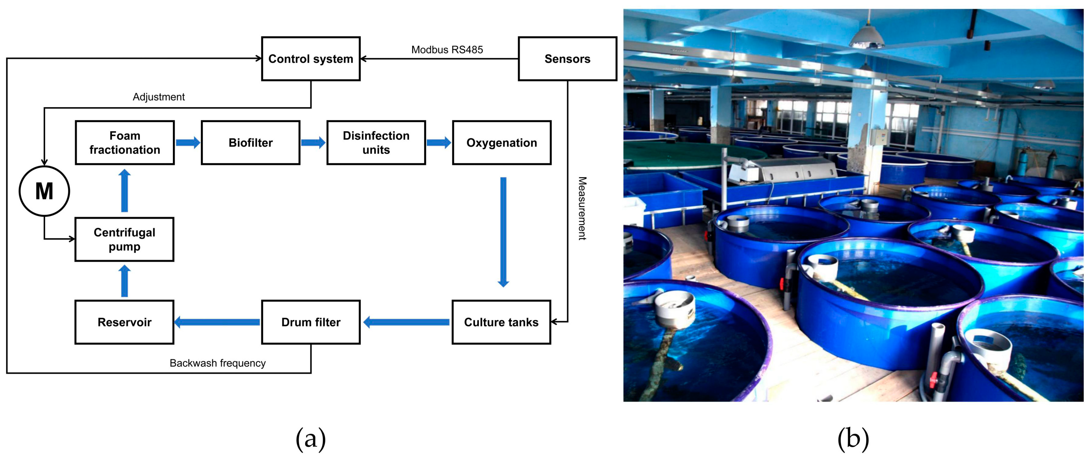
The experimental RAS used the recirculating aquaculture system of Dalian Huixin Titanium Equipment Development Co., Ltd. (Dalian city, China) for breeding
L. vannamei. Figure 1a shows the schematic of the experimental RAS control system. The control system collected the water quality indicators by connecting them with the sensors. Water quality changes can be monitored in real time, and the centrifugal pump was controlled by variable-frequency operation using a flow regulation model based on machine learning. The variable-flow circulation caused different trends in the drum filter backwash frequency during the unit period (0.5 h). The water quality indicators were used to train the regulation strategy model for variable-flow circulation. The types of water treatment equipment included biofilters, a micro-screen drum filter, an ultraviolet generator, ozone generators, foam fractionators, and oxygenation cones.
Figure 1b shows the actual indoor workshop. The RAS contained 10 circular FRP tanks with a diameter of 1.8 m and a depth of 1.4 m, with a total water volume of 35 m
3. Shrimp were fed five times a day during the culture period with a 36% protein commercial feed (Dale 2# shrimp commercial feeds, Dale, Inc., Yantai, China). During the early stage of shrimp culture, the amount of feed accounted for 5–8% of the total biomass of shrimp. The amount of feed was reduced over time and accounted for 3.7–5% of the total biomass by the end of the culture process. The whole culture process lasted for 90 days, with a culture density of 800 individuals/m
3 and a final yield of 525 kg of shrimp.
2.2. Variable-Flow Experiment Design
Turbidity (NTU) is mainly influenced by water flow fluctuations and can only reflect the instantaneous transparency of the water body. This study proposes a technique for detecting turbidity in an RAS based on a micro-screen drum filter. The backwash frequency of the drum filter within a unit period (0.5 h) was used to represent overall RAS turbidity, and the variable-flow regulation model was constructed using the backwash frequency and various water quality data. The variable-flow regulation model can determine the operating frequency of the centrifugal pump for the next period using real-time data from the current period. The intelligent variable-flow RAS technology is implemented by controlling the RAS circulation rate by changing the circulating pump flow rate. The primary purpose of the variable-flow RAS is to implement a linkage control technology to model the relationship between the micro-screen drum filter backwash frequency and the circulation flow rate.
The total flow rate of the circulating pump was set to three levels: 55, 65, and 75 m3/h. The circulation rate was operated with a cycle of 24 h. A cycle started with a circulation rate of 55 m3/h and was adjusted to 65 m3/h after an interval of 24 h and then to 75 m3/h after the same interval (24 h). The drum filter controller collected backwash data every 0.5 h. Turbidity sensors were placed at the main return pipeline to monitor and record overall RAS water turbidity. Water quality indicators, including water temperature (T), dissolved oxygen (DO), pH, and salinity, were measured by sensors in real time using YSI ProPlus portable sensors. Total suspended solids (TSS), total ammonia nitrogen (TAN), and nitrite nitrogen (NO2-N) were measured daily with a Palintest 7500 water quality analyzer.
The circulating pump was set to three circulating levels: slow (55 m3/h), medium (65 m3/h), and fast (75 m3/h). In the variable-flow RAS, the circulation rate was maintained at a medium level, and the control system read water quality indicators and backwash times from sensors at every unit period. The circulation rate for the next period could be adjusted to slow or fast levels. The circulation adjustment process could be operated in two ways: upshift and downshift. In the drum filter controller program, the backwash frequency was recorded for 48 periods in a day, using 0.5 h as a period. The circulating pump was utilized to determine the upshift/downshift for the next period by reading the current water quality sensors, current backwash frequency, and current circulating level. A water gauge controlled the drum filter backwash frequency; the backwash frequency reflects water turbidity in the RAS. Downshifts (−1) and upshifts (+1) of circulating pump frequency were used as indicators of circulation levels. The water quality indicators, current circulating pump frequency, and the drum filter backwash frequency were chosen as independent variables, and the downshifts (−1)/upshifts (+1) data were considered as the dependent variable. As the whole culture process lasted for 90 days in the RAS, the total circulation rate was set to 55 m3/h for the first 30 days, 65 m3/h for the middle 30 days, and 75 m3/h for the last 30 days. Establishing a variable-flow circulation strategy was the core task of the experiment, and therefore the circulation rate regulation model was constructed using the optimal classification model based on machine learning to control the variable-flow circulation rate in the RAS.
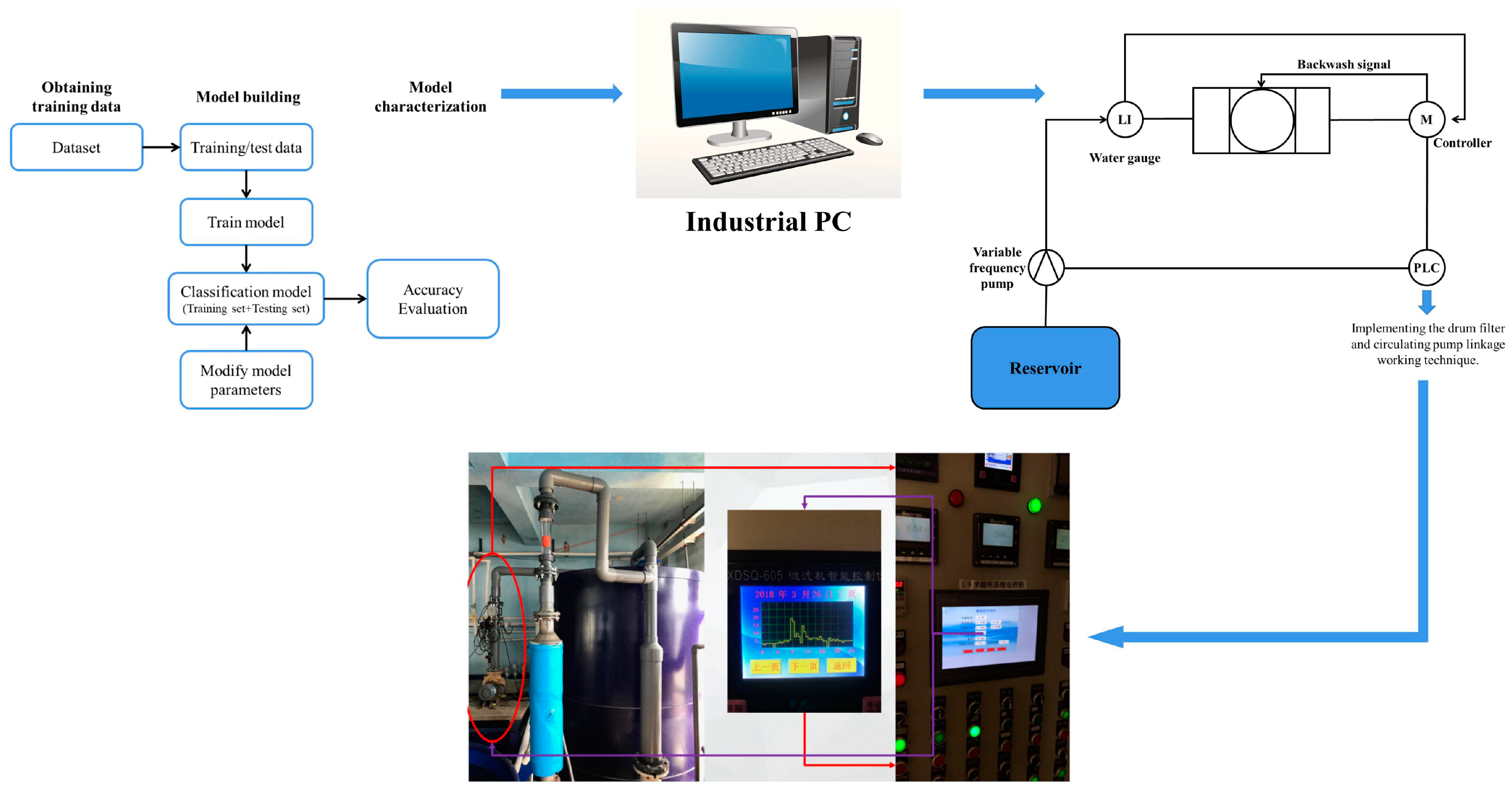
As shown in
Figure 2, the drum filter controller was used to collect the backwash frequency, circulation flow rate, and water quality data that were then uploaded to the industrial PC through the RS485 protocol. The embedded system was connected to the industrial computer. The dataset was processed with the optimal machine learning model in the industrial computer to regulate pump frequency for the next period and feed it back to the embedded system, so that the RAS circulation flow rate could be regulated intelligently.
2.3. Machine Learning Methods
2.3.1. Artificial Neural Networks (ANNs)
ANNs are statistical learning algorithms that possess prediction and approximation abilities given sufficient and considerable inputs [
26]. ANNs are derived from the biological neural networks in the human brain. Interconnected artificial neural networks are usually composed of neurons that can deal with the inputs and follow various situations. ANNs are suitable not only for machine learning but also pattern recognition. Therefore, ANNs have become a popular way of indicating a function by observation in the case of complex data.
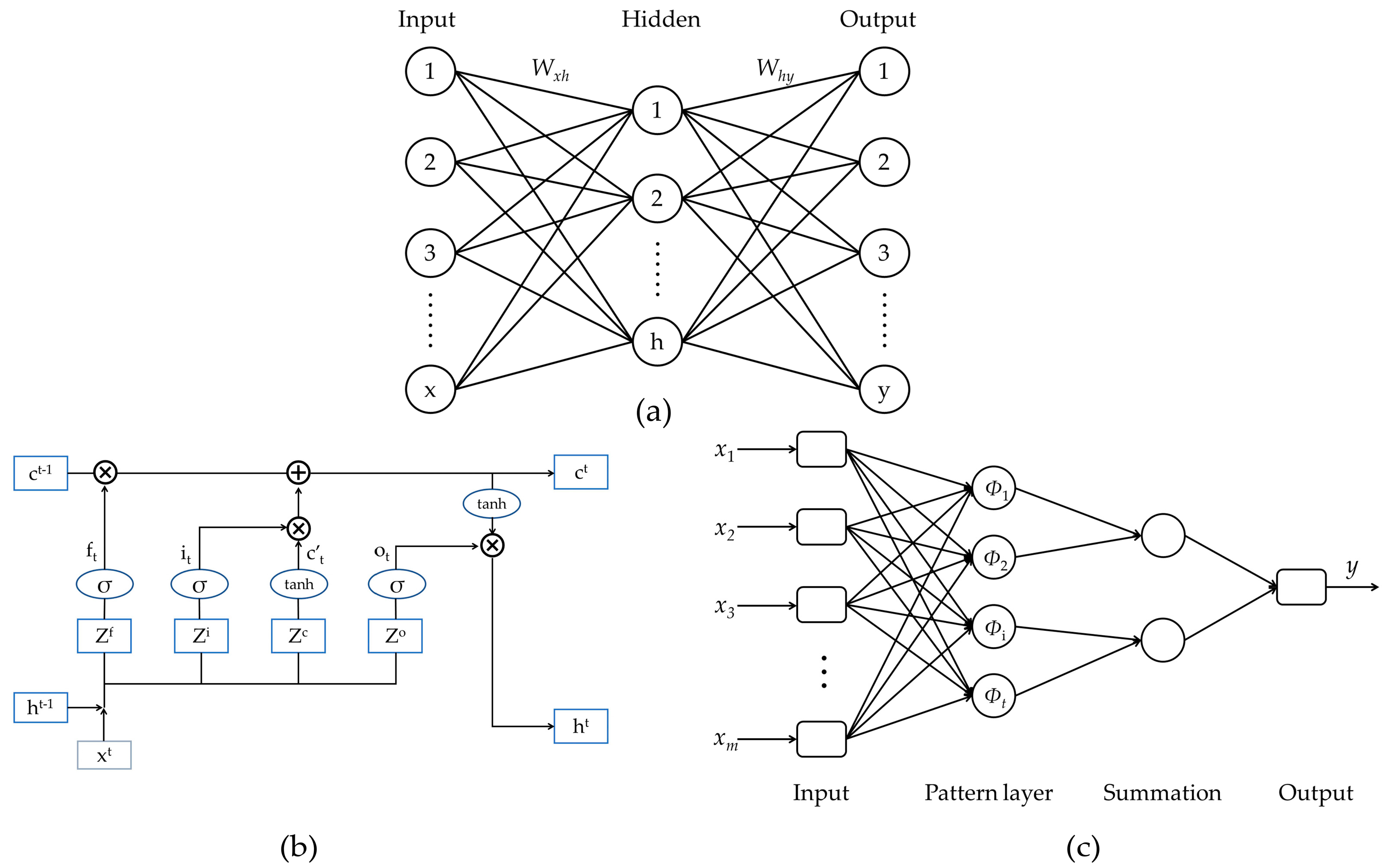
Figure 3a shows a typical ANN structure, including input, hidden, and output layers.
In this study, several ANN methods, including the backpropagation neural network (BPNN), extreme learning machine (ELM), probabilistic neural network (PNN), and long short-term memory (LSTM) neural network, were used to develop variable-flow models. The BPNN and ELM are feedforward neural networks with no cycles or loops. Information propagates in one direction, forward from the input layer, through the hidden layer, and then to the output layer, in a feedforward neural network.
The activation function can introduce a nonlinear factor to the neuron so that the ANN can approximate any nonlinear function. In the present study, a sigmoid function was adopted in the BPNN model and ELM model. For the sigmoid activation function, it holds that
where the output of the sigmoid function is between 0 and 1. For the binary classification task, the output of the sigmoid is divided into a positive class/negative class when the output satisfies a certain probability condition.
Figure 3b shows the schematic of the LSTM network. The LSTM network is a special RNN focusing on long sequences of data [
27]. A standard LSTM unit comprises a cell, an input gate, an output gate, and a forget gate to solve the long-term dependency problem. Long-term memory information is stored during three steps (forgetting, remembering, and outputting) in an LSTM. In the present study, a rectified linear unit (ReLU) function was applied in the LSTM model. The ReLU function is described as
which means that
The convergence rate of the stochastic gradient descent obtained by the ReLU function is much faster than the tanh/sigmoid function. However, the learning rate should be set appropriately to prevent neurons in the network from losing their activation ability. In this study, the parameters of the LSTM training process were set as follows: sequence input layer = 9, initial learning rate = 0.01, learning rate drop factor = 0.1, batch size = 128, number of training epochs = 200, hidden layer = 1 (with 32 hidden units). Adaptive moment estimation (Adam) was chosen as the optimization method. The fully connected layer was set as 2 for the binary classification task.
Figure 3c shows the architecture of a typical PNN, which was first proposed by Dr. D.F. Specht [
28]. As a branch of a radial basis network, PNN has the advantages of a simple learning process and fast training time. Therefore, PNN models can be well implemented in hardware since the neuron number in each layer is fixed. Generally, a PNN network contains four layers: input layer, pattern layer, summation layer, and output layer. The input layer simply distributes the input to the neurons in the pattern layer. The pattern layer neuron may compute its output by Gaussian function when receiving
x from the input layer. It holds that
where
lg denotes the total number of samples,
n is the input feature, sigma represents the smoothing parameter, and
xij represents the
j-th data of the
i-th neuron of the class
g. The summation layer connects the pattern layer units of each class, and then the output layer is responsible for outputting the category with the highest score in the summation layer. K-fold cross-validation is useful for preventing models with small datasets from overfitting but is not used too frequently in deep learning. The dataset is equally divided into k parts. Every time a unique fold is used as a validation subset, the remaining pattern examples train the ANN. In this study, we introduced 4-fold cross-validation to evaluate the machine learning models. The evaluation indicators were all calculated by averaging the 4-fold cross-validation results.
2.3.2. Support Vector Machine (SVM)
An SVM has excellent generalization ability between model complexity and learning ability when dealing with limited sample information [
29]. In SVM applications, choosing the appropriate kernel function and suitable parameters is crucial for prediction accuracy. As for the linear separable binary classification, finding the optimal hyperplane that divides all samples with maximum margin is the principal function of an SVM. For linear problems, the optimal classification hyperplane in separating two classes of training vector sets
D is
When the optimal classification surface is generated, the vectors are classified without error, and when redundancy occurs, a typical hyperplane is assumed where
w and
b are constrained:
The classification hyperplane in the regular form must satisfy the following constraints:
The coordinate of the point
x in the hyperplane at a distance
is
The final hyperplane that can satisfy the separated samples is the hyperplane that minimizes the data:
For nonlinear classification, the idea of SVM is to map the samples to a high-dimensional space, where the nonlinear problem is transformed into a linear solution using a kernel function, at which point the weight
w is expressed as
Introducing the relaxation variable
describing the function interval, the optimization equation under the kernel approach is expressed as
The model is described as
In the present study, the SVM model was adopted to control the inverter frequency to improve circulating pump operating efficiency under different water quality conditions. The SVM is a kind of machine learning algorithm with a high generalization ability to classify and predict small samples. As upshifting and downshifting of the circulating pump is a binary problem, water quality indicators as variables can provide good generalization ability for the model. Support vector classification (SVC) can be used as the core algorithm for developing drum filter-circulating pump linkage technology. However, there is no international standard for selecting optimal parameters, and the parameter selection principles are based on dataset performance and the construction of a more reliable solution through cross-validation methods [
30,
31]. Here, we used the Gaussian kernel function in resolving the nonlinear support vector classification task:
For the SVM model, the penalty parameter C and RBF kernel parameter g need to be decided to improve the classification accuracy. In the present study, several optimizing algorithms, including grid search (GS), least squares method (LS), genetic algorithm (GA), and cuckoo search (CS) algorithm, were applied to improve the classification performance of the SVM model. The parameters of GA were set as follows: max generation = 300, population size = 50, generation gap = 0.9, range of parameter c = (0, 100), range of parameter g = (0, 1000). For the CS algorithm, the parameters were set as follows: iteration = 300, number of nests = 20, probability = 0.25. The best parameters of GS and LS methods were obtained through the traversal method; the ranges of c and g were set as (0, 100) and (0, 1000), respectively. K-fold cross-validation was utilized in the SVM models to prevent overfitting, and the evaluation indicators were calculated using averaging. The optimal SVM model can be determined by comparing the evaluation indicators of classification results from different algorithms.
4. Discussion
Feces and residual feed may decompose to organic suspended solids, which further generate TAN and nitrite, harming breeding animals’ health. Suspended solids in the RAS also provide surface area that can be colonized by bacteria. As circulation intensity increases, more particles accumulate, which may increase the bacterial carrying capacity of the system. Hence, rapid removal of solid waste is the most critical unit process in an RAS [
34]. The traditional method of water quality regulation in an RAS is to act when water quality deteriorates. This approach leads to large fluctuations in the water environment, and the cost of water quality regulation becomes very high, often requiring many water exchanges to control water quality. This study proposes regulation of RAS circulation based on process control technology, relying on the microfilter backwash times in a unit period (0.5 h) as the main parameter to reflect the overall turbidity of the water body. The variable-flow RAS circulation strategy was designed to form microfilter-circulating pump linkage technology based on water quality parameters and backwash times at different flow rates. An intelligent variable-flow regulation model was developed to keep the water clean and quickly and dynamically remove suspended solids.
Related research has proven the significant differences in water quality between the high and low makeup water exchange treatment groups [
35]. One study has shown that increasing RAS water circulation can effectively reduce ammonia and nitrite [
36]; the higher the circulation level, the lower the ammonia and nitrite mass concentrations became. Moreover, the conversion of nitrite revealed a certain hysteresis, and the ammonia peak appeared earlier than the nitrite peak after feeding was stopped.
RAS solids come mainly from uneaten feed and fecal solids, and the decomposition and mineralization of these solids lead to elevated ammonia and nitrite levels in the RAS [
10]. Data such as TAN, NO2-N, and TSS must be obtained by manual measurement and are challenging to obtain by sensors. According to Vinatea et al. [
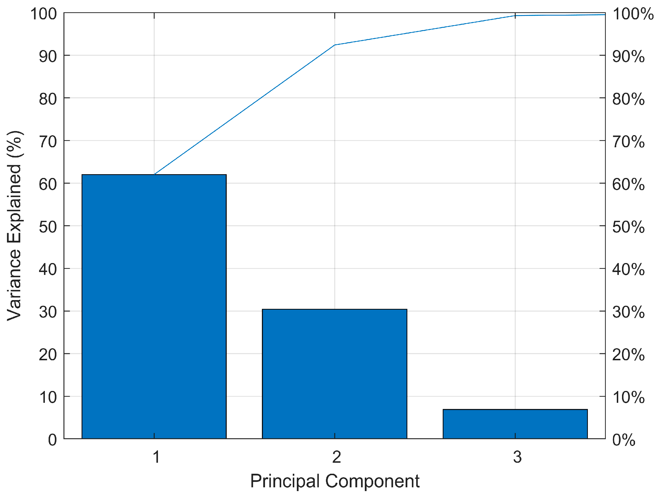
37], TSS tended to accumulate in the intensive
L. vannamei culture and was eventually reflected in an increase in NTU. As both turbidity and TSS can reflect the clarity of a liquid, the turbidity parameter was used for modeling in this study. The principal component analysis (PCA) results for dimensionality reduction showed that turbidity, dissolved oxygen, pH, and temperature could be used as the leading indicators for modeling. The variable-flow regulation model obtains the current water quality indicators in real time and then applies these indicators to predict and classify the circulation rate for the next period. The turbidity sensor in turbulent flow had a measured data fluctuation that was too large, and the sensor arrangement position also caused measurement errors. An innovative point of this study is that the drum filter backwash frequency over a certain period was used as one of the critical factors for modeling instead of the momentary RAS water turbidity. Backwash times can effectively replace turbidity reading to reflect overall RAS water turbidity, avoiding the instability of the data collected by the turbidity sensor.
The application of machine learning methods in aquaculture-related research is focused mainly on the prediction, classification, and evaluation of water quality indicators such as dissolved oxygen, salinity, pH, ammonia, and nitrite [
25]. In the present study, machine learning was used to model the variable-flow regulation strategy. Sensors collected water indicators, including DO, pH, temperature, and turbidity. In order to implement the variable-flow principle, the machine learning methods were introduced in the present study to develop the optimal variable-flow regulation model for RAS. The water quality indicators, the backwash frequency, and the circulating pump frequency were obtained through continuous monitoring. For the ANN methods, the LSTM model was identified as the optimal regulation model, since the accuracy and F1-score indicators reflected the strong ability of the LSTM classifier. The modeling data based on time series were collected from the continuously running RAS in the present study. The water quality indicators, backwash frequency, and total circulation rates were recorded through the fixed time interval during the whole rearing period. Research has shown that LSTM can indeed perform well in processing long time series sequences of data [
38]. The optimal classification model needs to be relatively simple in order to be applied in the embedded devices. The variable-flow adjustment strategy in RAS also needs to respond quickly and satisfy the high standard of classification accuracy. All the evaluated indicators of the SVM models demonstrated better results compared with the LSTM model. The gene algorithm contributed the highest accuracy and F1-score among the four optimization algorithms in the classification task. As a supervised algorithm, GA-SVM can be applied to effectively adjust water refreshment in RAS.
In future work on variable-flow RAS regulation, the data-driven model needs to be improved to establish continuous variable-flow control technology by adjusting circulating pump frequency. A larger quantity of data from the running RAS can ensure higher availability and robustness for optimizing the intelligent variable-flow strategy. The continuous variable-flow control technology prerequisite is required for the indicators (water quality, backwash frequency, and rearing cycle) to correspond to the ideal circulation volume. Furthermore, the interaction effects between various indicators need to be revealed through experiments and analysis. The ultimate goal of the study is to achieve a precise circulation control strategy in the RAS and execute rapid water treatment without affecting the health of the reared animals.
5. Conclusions
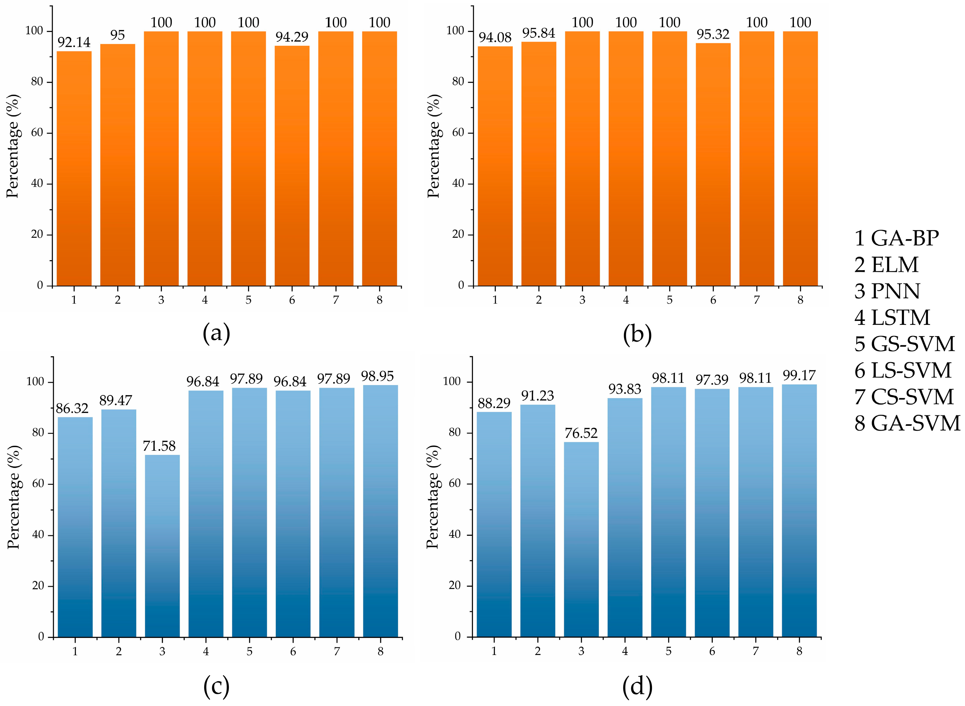
A variable-flow regulation model was established in the present study to implement the circulating pump-drum filter linkage working technique. Classification models based on machine learning methods between the explanatory variables and the regulation strategy were developed based on experimental data. ANN models including GA-BP, LSTM, PNN, and ELM were established. The LSTM model had the highest accuracy (training set 100%, test set 96.84%) and F1-score (training 100%, test 93.83%) and was regarded as the best classification model among ANN methods. SVM models were developed and optimized using linear squares, grid search, cuckoo search, and gene algorithm. Results showed that SVM models required less training time and exhibited higher accuracy compared with ANN models. Finally, the optimal model was GA-SVM, with the highest classification accuracy (training 100%, test 98.95%) and F1-score (training 100%, test 99.17%). The model was tested under cross-validation with precise classification performance and used for the circulating pump-drum filter intelligent linkage working technique.


