Article

An Expert Artificial Intelligence Model for Discriminating Microseismic Events and Mine Blasts

1
School of Resources and Safety Engineering, Central South University, Changsha 410083, China
2
China Nonferrous Metals Int’l Mining Pakrut LLC, Beijing 100029, China
3
NFC Africa Mining PLC, Kitwe 22592, Zambia
*
Authors to whom correspondence should be addressed.
Appl. Sci. 2021, 11(14), 6474; https://doi.org/10.3390/app11146474
Submission received: 10 June 2021 / Revised: 6 July 2021 / Accepted: 8 July 2021 / Published: 13 July 2021
(This article belongs to the Topic Applied Computer Vision and Pattern Recognition)

Abstract

:
To reduce the workload and misjudgment of manually discriminating microseismic events and blasts in mines, an artificial intelligence model called PSO-ELM, based on the extreme learning machine (ELM) optimized by the particle swarm optimization (PSO) algorithm, was applied in this study. Firstly, based on the difference between microseismic events and mine blasts and previous research results, 22 seismic parameters were selected as the discrimination feature parameters and their correlation was analyzed. Secondly, 1600 events were randomly selected from the database of the microseismic monitoring system in Fankou Lead-Zinc Mine to form a sample dataset. Then, the optimal discrimination model was established by investigating the model parameters. Finally, the performance of the model was tested using the sample dataset, and it was compared with the performance of the original ELM model and other commonly used intelligent discrimination models. The results indicate that the discrimination performance of PSO-ELM is the best. The values of the six evaluation indicators are close to the optimal value, which shows that PSO-ELM has great potential for discriminating microseismic events and blasts. The research results obtained can provide a new method for discriminating microseismic events and blasts, and it is of great significance to ensure the safe and smooth operation of mines.

1. Introduction

As the exploitation and utilization of mineral resources and underground space have entered deeper into the earth, rock bursts and other ground pressure disasters have become more and more frequent, so the safety of deep geotechnical engineering has attracted more and more attention [1]. The microseismic monitoring system has the characteristic of real-time monitoring. It can effectively monitor the micro-fracturing inside the rock mass which may expand into macroscopic instability and failure, and the failure evolution process inside the rock mass can also be revealed by it. People can obtain the precursors of ground pressure disasters based on the monitored microseismic data, and take appropriate measures in time to avoid hazards to personnel or equipment, which is of great significance in the smooth progress of the project. Therefore, it has been widely applied in underground mines [2,3], the slope of hydropower stations [4,5], underground caverns [6,7] and tunnels [8,9].
Due to the complexity of the on-site environment of mining activities in mines [10], the monitored microseismic signals tend to be mixed with other signals, including blast signals, drilling signals, electrical signals and mechanical vibration signals [11]. At present, discriminating signal categories is usually done manually, which not only requires an operator with extensive practical experience and deep professional knowledge [1], but also causes problems such as a heavy workload of discriminating events, strong subjectivity due to it depending on an operator’s experience, and delays in discriminating results [12]. In addition to the blast signal, other interference signals mentioned above have a significant difference in waveform from the microseismic signal, and so it is relatively easy to distinguish them from microseismic signals. However, for the blast signal, its waveform is very similar to the microseismic signal, which greatly increases the probability of misjudgment in manual discrimination. Therefore, an efficient and reliable method is urgently needed for discriminating the huge number of microseismic records in mines.
Researchers worldwide have conducted many studies to differentiate seismic events from human-made explosions, including nuclear explosions and mining blasts [12,13], and many different techniques have been proposed. For example, Derr [14] discriminated earthquakes and underground explosions in the Western United States by means of the Rayleigh-wave spectral ratio of short- to long-period energy, which belongs to the waveform spectrum analysis method. Zeiler et al. [15] used magnitude and amplitude ratios to discriminate small earthquakes and blasts at local distances, and obtained a good discrimination performance. Kim et al. [16] used the method based on the spectral amplitude ratio of the vertical components of P-waves and S-waves in a specified frequency range to discriminate earthquakes and blasts. Ford et al. [17] utilized aftershock characteristics to differentiate explosions from earthquakes. Among them, artificial intelligence techniques are widely reported and effective, and have been used in many other fields, such as the prediction of blast-induced rock movement [18], the optimization of postblast ore boundary determination [19], the prediction of rockbursts [20], the prediction of blast-induced air overpressure [21], and the prediction of the strength of the fiber-reinforced cemented paste backfill [22].
For signal discrimination, support vector machines [23], neural networks [13], logistic regression [24], hidden Markov models [25], the Gaussian classifier [26], the Fisher classifier [27] and the naive Bayesian classifier [28] have been widely applied. Usually, some characteristic parameters obtained from the events are selected to represent the original signal and then are used as the input parameters of the models established by intelligent algorithms to discriminate events. For instance, Kortström et al. [23] proposed an automatic classification method for seismic records in areas with few seismographs which makes use of support vector machines (SVM). According to this method, the seismic records are divided into four phase windows after they were filtered by 20 filters. Subsequently, the short-term averages of all filter channels and phase windows are computed. The dataset consists of 80 parameters that play the role of training the SVM model will be assigned to each event station pair. Vallejos and McKinnon [24] adopted logistic regression and neural network classification techniques to classify seismic records based on 14 parameters obtained from the ESG microseismic monitoring system and achieved a relatively high classification accuracy. Bui Quang et al. [25] presented a new method for the detection and classification of seismic events at an array station which combined the progressive multi-channel correlation detector and a statistical time series classifier based on hidden Markov models. Malovichko [26] used a multivariate maximum-likelihood Gaussian classifier technique to discriminate microseismic events and mine blasts. It utilizes four seismic event characteristics and quantifies a probability that a particular event belongs to a population of blasts. Zhao et al. [27] chose spectral characteristics, the event time in hours and two physical characteristics of waveforms as discrimination features, and then developed a model based on statistics through the use of Fisher discriminant analysis which achieved a high discrimination accuracy. Dong et al. [28] selected nine ratios of the energies contained within predetermined velocity windows and average distance as feature parameters and then uses nonlinear methodologies including naive Bayesian classifier to discriminate seismic events and nuclear explosions. Shang et al. [13] adopted an artificial neural network for the classification of microseismic events and mine blasts. Twenty-two seismic parameters from the microseismic monitoring system were selected as characteristic parameters, and the effect of each parameter on classification was analyzed by principal component analysis.
However, the discrimination accuracy of some of the above intelligent algorithms is not very high, and there is still potential for improvement. In addition, no algorithm is suitable for all problems and all field sites are based on the well-known ‘no free lunch’ theorem, and the combination of the extreme learning machine and the particle swarm optimization algorithm has not been used to discriminate seismic events and blasts. In this paper, an artificial intelligence model called PSO-ELM based on the extreme learning machine optimized by the particle swarm optimization algorithm is applied to discriminate microseismic events and blasts in underground metal mines. In order to check the discrimination performance of PSO-ELM, experiments were also carried out with the original extreme learning machine model and other commonly used intelligent discrimination models, including the backpropagation neural network, the naive Bayesian classifier and Fisher discriminant analysis. All the algorithms were implemented in MATLAB R2016b. The discrimination performance of the five intelligent discrimination models above is compared and analyzed. The research results obtained can provide a new method for the discrimination of microseismic events and blasts, and this is helpful to promote the safe and smooth operation of mines.

2. Data

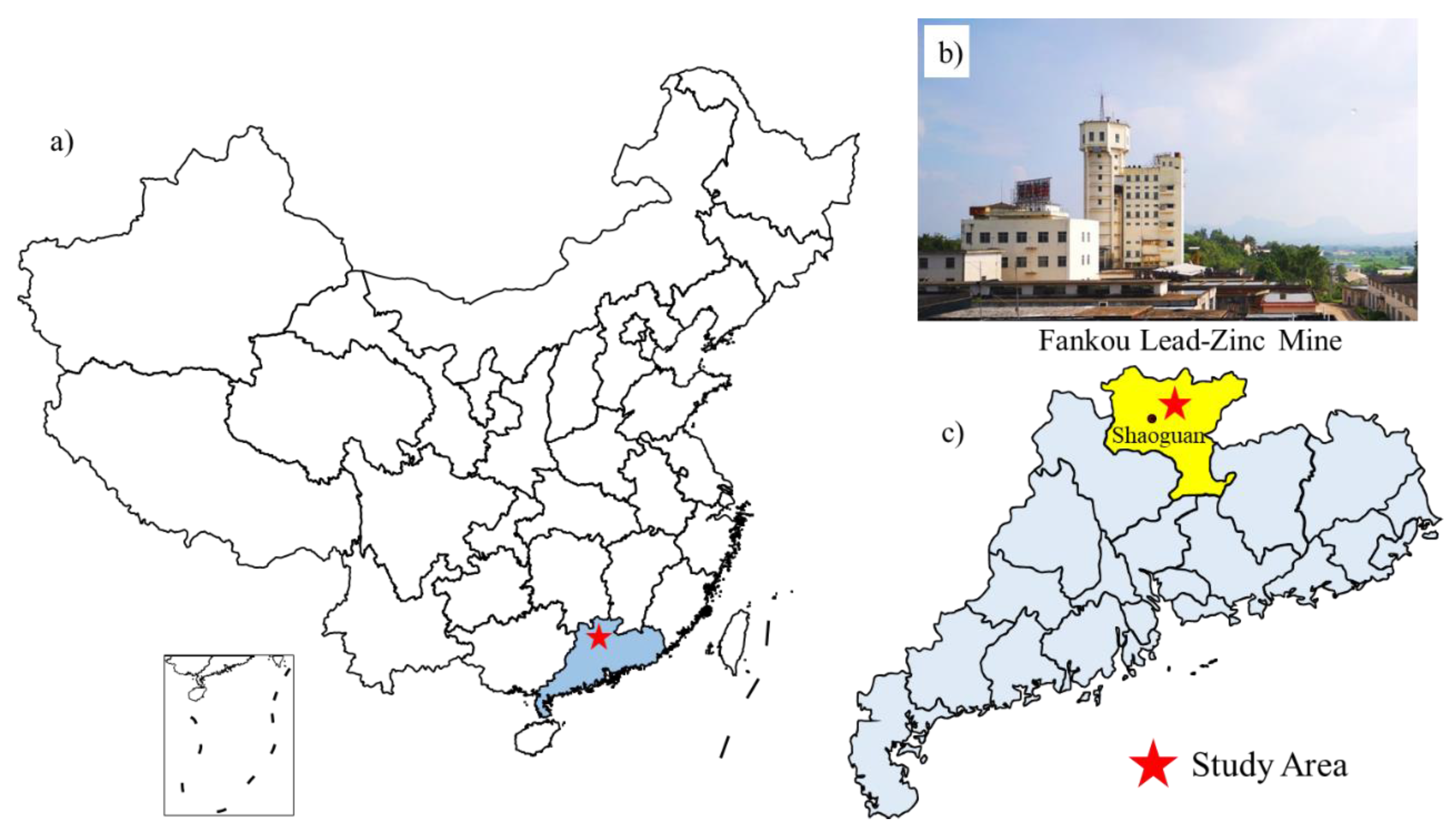
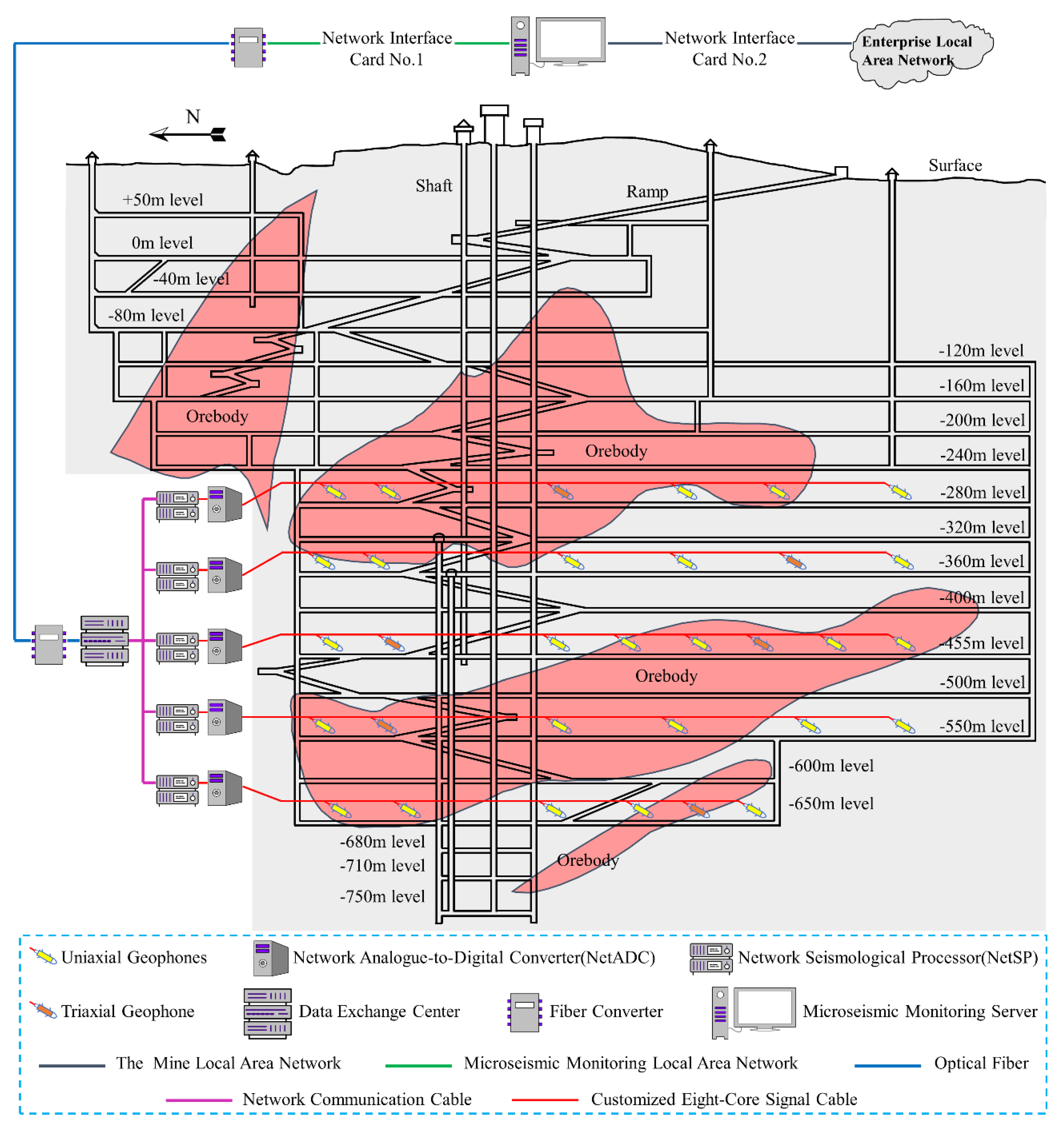
2.1. Outline of the Mine and Microseismic Monitoring System

The experimental data were obtained from Fankou Lead-Zinc Mine (see Figure 1) in Shaoguan, Guangdong Province, China, using the Institute of Mine Seismology (IMS) system, which was installed in 2016. Two mining methods, the large-diameter longhole (LDL) mining method and the upward horizontal cut and fill stoping method, are used to extract the ore underground. The deepest mining depth is close to 900 m underground. The IMS system contains 6 triaxial geophones and 26 uniaxial geophones (see Figure 2), which are distributed at five levels of −280, −360, −455, −550, and −650 m. Both triaxial and uniaxial geophones hold a natural frequency of 14 Hz, and their frequency response is 9 to 2000 Hz.
The continuous voltage signal is recorded by the geophone and then transmitted to the eight-channel network analogue-to-digital converter (NetADC) via the customized eight-core signal cable for analog-to-digital conversion—that is, the analog signal is sampled by NetADC at a 6000 Hz sampling frequency to be converted into a digital signal. Then, the network seismological processor (NetSP) performs noise reduction and amplification processing on digital signals. After that, the signal data from each NetSP are transmitted to the data exchange center through the network communication cable, and are modulated into an optical signal by the fiber converter. Finally, the signal data are transmitted to the microseismic monitoring server on the ground through the optical fiber, so as to realize event location, statistics, analysis of rock mass stability, etc.

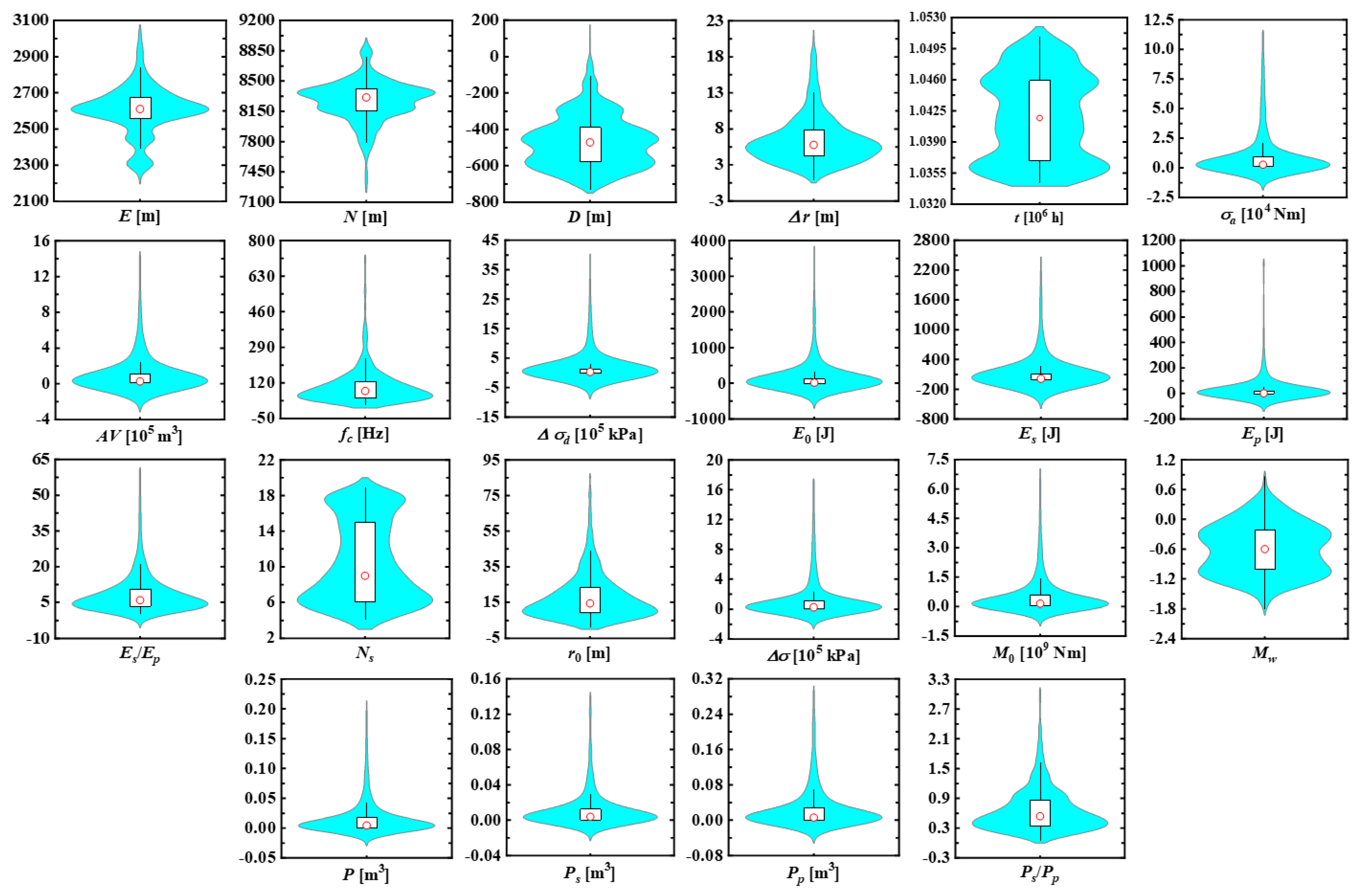
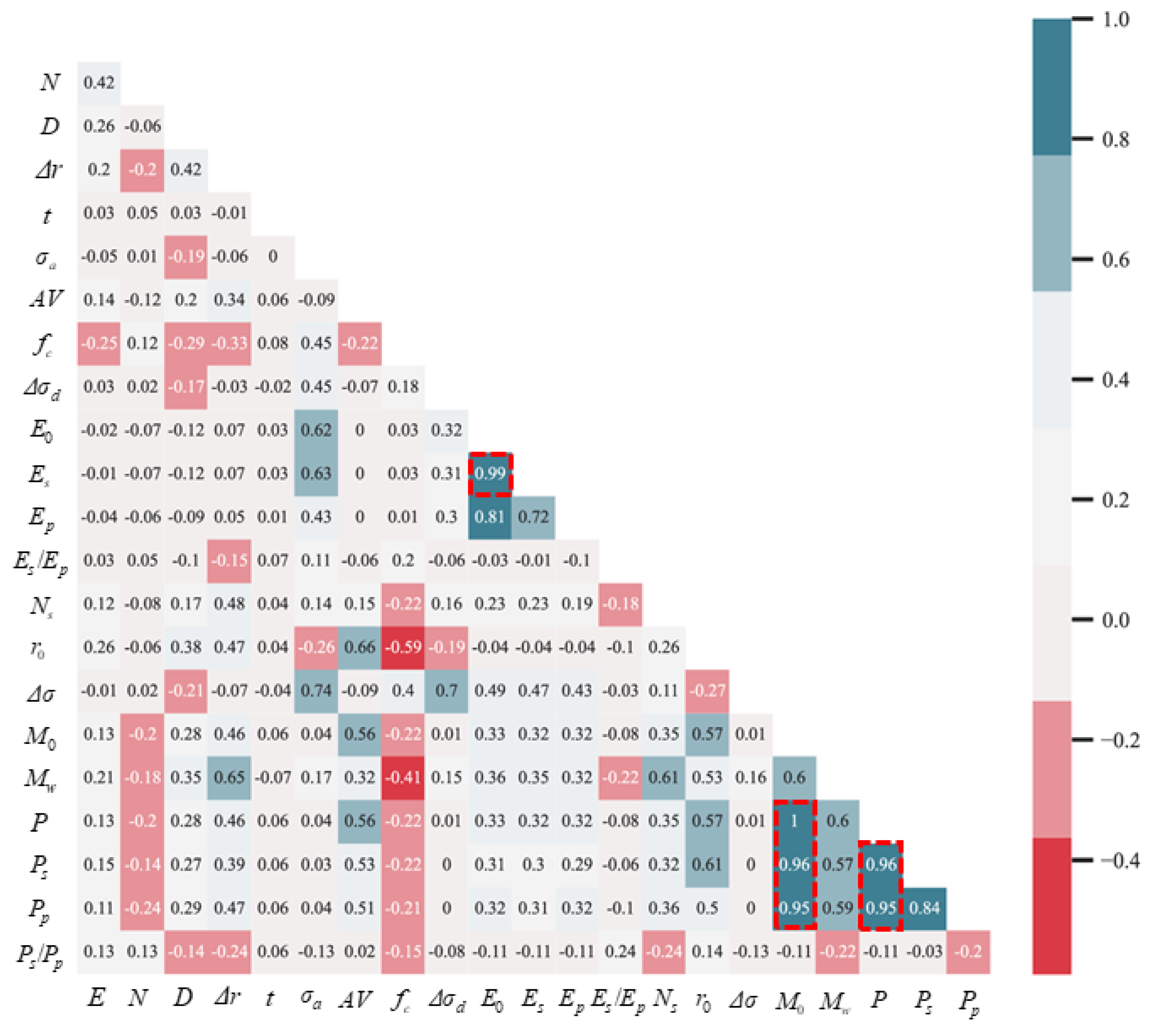
2.2. Discriminant Parameters and Sample Dataset

The microseismic event can be regarded as the sudden release of potential or stored energy in the rock, which is then radiated in the form of seismic waves [29,30]. Development or production blasting in mines is a rapid chemical reaction of an explosive substance which causes crushing and fracturing in the surrounding rock mass or the cemented paste backfill [31,32]. It initiates a disturbance that propagates outwards, predominantly in the form of a compressional seismic wave [26]. Blasts or explosions usually radiate waves of higher frequency than microseismic events [33], and various combinations of seismic parameters, such as the ratio between seismic moment and corner frequency, apparent stress, etc., can be used to obtain the difference in frequency components between blasts and microseismic events [26]. The seismic wave radiation pattern of microseismic events is also different from that of blasts. A blast radiates predominantly P-waves from the source, while the microseismic event caused by shear cracking or slip on a contact face radiates P-waves that are weaker than S-waves [26,30]. The amplitude relationship between P-waves and S-waves can be obtained by comparing M p with M s , which are the seismic moments estimated based on P-waves and S-waves, respectively. This means that the ratio of M s to M p and its equation, such as the ratio of P s to P p , can be used as the characteristic parameters of the seismic wave radiation pattern, where P s and P p are the total potency of S-waves and P-waves, respectively. In addition, generally, mines conduct blasting operations within a relatively fixed period of time. Therefore, an event that occurred during this period of time is more likely to be a blast than a microseismic event [26]. Based on the above differences between blasts and microseismic events, and combined with previous research results [13,24], 22 seismic parameters, including the longitudinal direction coordinates of the event location (E), the latitudinal direction coordinates of the event location (N), the depth direction coordinates of the event location (D), the associated vectorial error sum ( Δ r ), the origin time of seismic records (t), apparent stress ( σ a ), apparent volume (AV), corner frequency ( f c ), dynamic stress drop ( Δ σ d ), total radiated energy ( E 0 ), S-wave radiated energy ( E s ), P-wave radiated energy ( E p ), S-wave to P-wave energy ratio ( E s / E p ), the number of sensors used in the location of the event ( N s ), the source radius ( r 0 ), static stress drop ( Δ σ ), seismic moment ( M 0 ), moment magnitude ( M w ), the total potency of the P- and S-wave ( P ), the total potency of the S-wave ( P s ), the total potency of the P-wave ( P p ) and the S-wave to P-wave potency ratio ( P s / P p ), were selected as the preliminary characteristic parameters for discriminating microseismic events and blasts in this work. One thousand six hundred events, 50% of which were microseismic events, while the remaining 50% were blasts, were randomly chosen from the IMS database as the sample dataset to ensure the applicability of the PSO-ELM method to different microseismic signal data. These 1600 events were recorded from 2016 to 2020, and the number of events in the sample dataset is considerable, which is helpful in avoiding the overfitting phenomenon. The values of the above 22 parameters of the 1600 events were calculated with the help of the built-in software of the IMS system after the P-wave arrival picking and S-wave arrival picking performed manually on the recorded events, and their distribution is shown in Figure 3. The correlation coefficients between 22 seismic parameters are shown in Figure 4. Among them, the correlation coefficients between E 0 and E s , M 0 and P , M 0 and P s , M 0 and P p , P and P s , P and P p are 0.99, 1, 0.96, 0.95, 0.96 and 0.95, respectively, which are greater than the threshold value (0.85) suggested by Rovini et al. [34]. Maintaining one of the two or more parameters with a high correlation coefficient can reduce the amount of calculation and avoid overfitting. So, E 0 , P , P s , and P p were discarded, and the remaining 18 seismic parameters were adopted as the final characteristic parameters for discrimination in this paper. In addition, many researchers [35,36,37] suggest that the ratio of training data to testing data can be 8:2. Additionally, in this paper, 80% of the sample dataset was randomly allocated to the training set and the remaining 20% to the testing set.

3. Methodology

3.1. Backpropagation Neural Network (BPNN)

BPNN is a multi-layer feedforward neural network proposed in 1986 [1]. Its main structure comprises an input layer, one or more hidden layers and an output layer. The training process of BPNN includes two processes: signal forward propagation and error backpropagation. For the forward direction, the signal from the input layer is transmitted to the output layer through the hidden layer. If the actual output is different from the expected output, the error between the actual output value and the expected output value will be propagated back. Neural networks modify the weights of neurons by the sum of the squares of gradient descent on the errors. Training and adjustments are repeated in this way until the error between the actual output and the expected output reaches the minimum and is acceptable. After reviewing the previous study, BPNN has been used in many fields, including the path recognition of automated guided vehicles [38], air quality prediction and assessment [39], and stability analysis of underground mine hard rock pillars [40].

3.2. Naive Bayesian Classifier(NBC)

NBC is a discrimination technique derived from the probability model, which is a special form of Bayesian Network. It acquires the conditional probability of each attribute given a category label from the training data. Given an instance of a specific attribute, the Bayesian rule is used to calculate the category probability, and the category prediction is implemented by recognizing the category with the highest posterior probability [41]. The reason why this classifier is naive is that it assumes that the attributes are independent of each other. This assumption means that the conditional probability that an object to be classified belongs to a specific category given some attribute values has nothing to do with the values of other attributes [42]. Although this assumption is inconsistent with the reality, research by Domingos et al. [43] shows that it has no significant impact on the prediction performance of NBC. Moreover, a small amount of abnormal data will not greatly affect the results [44]. So, NBC has many applications, including tunnel face stability prediction [45], traffic accident duration prediction [42], and the classification of rockbursts in underground projects [46].

3.3. Fisher Discriminant Analysis (FDA)

FDA is a linear discriminant method proposed in 1936. It is a classic supervised learning method often used for dimensionality reduction and feature extraction. It projects the data points that are highly dimensional onto a low-dimensional space (such as a one-dimensional straight line) to make the data points denser and then determines the discriminant analysis function according to the principle of maximizing the distance between classes and minimizing the distance within classes, and finally classifies the new samples [47]. The primary target of FDA is to find the optimal linear approximation of the object feature vectors, which can be used effectively and reasonably in various classification tasks [48]. The discriminant performance of the FDA model is closely related to the information provided by the labeled dataset. It can separate the labeled training data into different categories by using the best projection vectors found by utilizing the label information [49]. FDA has been widely used in many areas including text classification [48], bioprocess monitoring [50], and predicting pillar stability for underground mine [51].

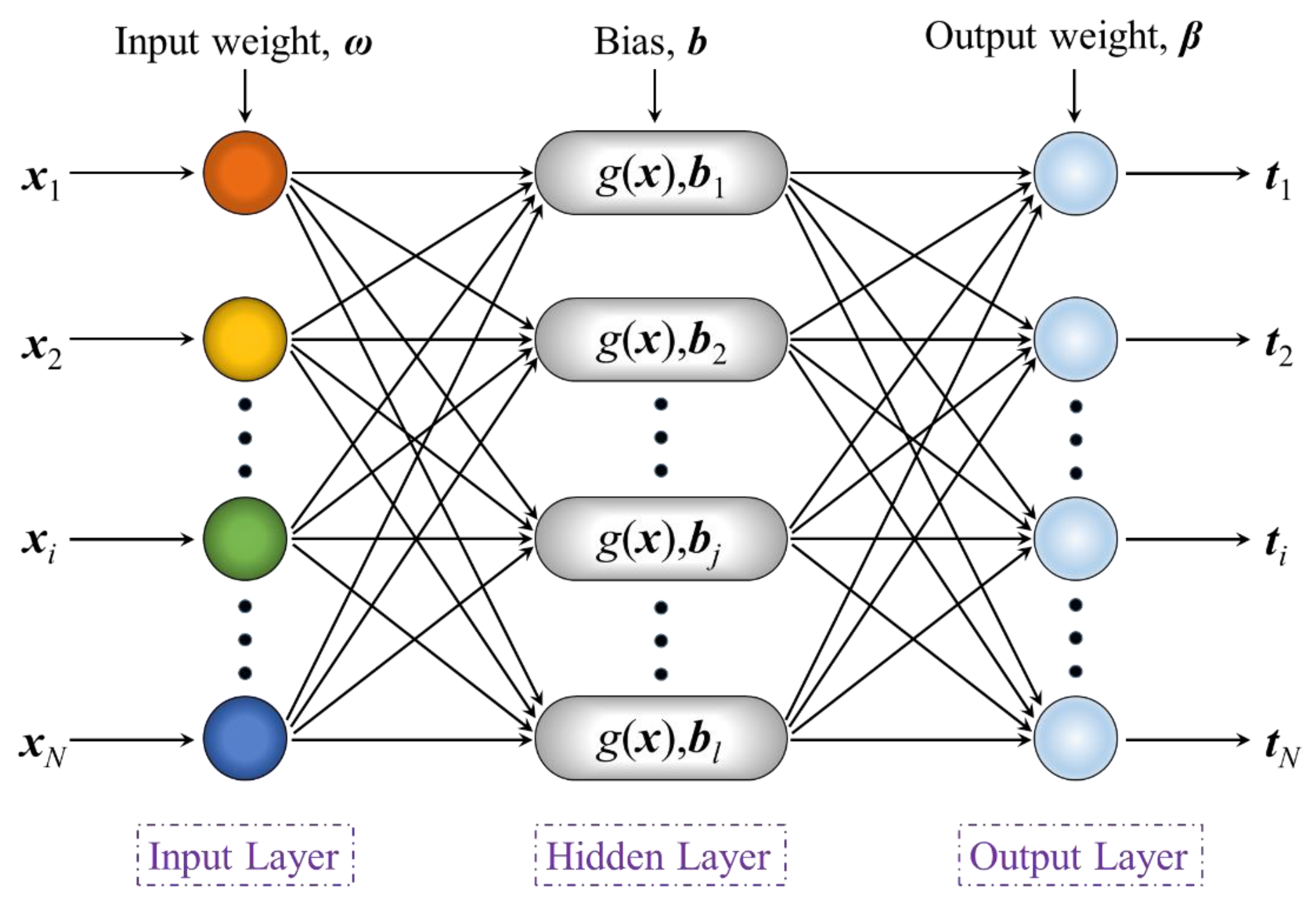
3.4. Extreme Learning Machine (ELM)

ELM was presented in 2004 by Huang et al., and belongs to the single-hidden layer feedforward neural network (SLFN) learning algorithms [52]. It can learn quickly with few training parameters, achieve good generalization, and has strong applicability [52]. ELM has the salient feature that the input weights and bias of hidden layer nodes (HLNs) are randomly generated using random algorithms and the only variable that needs to be calculated is the output weights, which is obtained through the least-square method. Therefore, compared with the conventional intelligent algorithms, it can learn faster while achieving better generalization [53].
Generally, an ELM network includes three parts: an input layer, a hidden layer and an output layer (see Figure 5). For N arbitrary different samples ( x i , t i ) , where x i = [ x i 1 , x i 2 , , x i n ] T R n , t i = [ t i 1 , t i 2 , , t i m ] T R m , a standard SLFN, of which the number of HLNs (NumHLNs) is l and the activation function is g ( x ) , can be expressed mathematically as follows [52,54]:
j = 1 l β j g ( w j x i + b j ) = o i
where i = 1 , , N and j = 1 , , l . w j = [ w j 1 , w j 2 , , w j n ] T is the input weight which connects the j th hidden node with the input nodes, β j = [ β j 1 , β j 2 , , β j m ] T is the output weight which connects the j th hidden node with the output nodes, b j is the bias of the j th hidden node, and w j x i is the inner product of w j and x i .
When the above standard SLFN infinitely approximates the N samples and the error is equal to 0, i.e., i = 1 N o i t i = 0 , there exist β j , w j , b j , so that:
j = 1 l β j g ( w j x i + b j ) = t i
The simplified form of Equation (2) is
H β = T
where
H ( w 1 , , w l , b 1 , , b l , x 1 , x N ) = [ g ( w 1 x 1 + b 1 ) g ( w 1 x N + b 1 ) g ( w l x 1 + b l ) g ( w l x N + b l ) ] N × l
β = [ β 1 T β l T ] l × m
T = [ t 1 T t N T ] N × m
where H is the output matrix of the hidden layer in ELM.
The difference between the ELM algorithm and the general SLFN algorithm is that the input weight w and hidden layer bias b of the former are given randomly at the beginning of the algorithm and accordingly calculating the output matrix H . Then, what needs to be done is to determine the parameter β . Training feedforward neural network can be regarded as seeking out the solution of H β = T by the least-square method. The output weight matrix β can be obtained through solving this equation:
β = H + T
where H + is the Moore–Penrose generalized inverse of H .

3.5. Particle Swarm Optimization (PSO)

PSO was presented in 1995 by Eberhart et al., belongs to the global optimization technique derived from the population [55], and has been applied in many fields, such as the evaluation of TBM tunneling rate [56], the evaluation and prediction of slope stability [57], and the prediction of ground vibration caused by blasting [58]. Its inspiration comes from the information-sharing behavior of social animals, such as birds. The PSO algorithm finds the best solution to the problem by sharing the information of the individuals in the swarm [54,59].
Suppose there are n particles in the space, the dimension of which is D , and they form a swarm. Each particle has two properties, position and speed, and the former stands for a possible solution to the problem. In the t th iteration, the position and the velocity of the i th particle are represented by x i ( t ) = [ x i 1 , x i 2 , , x i D ] and v i = [ v i 1 , v i 2 , , v i D ] , respectively. Whether a particle has reached a good position can be judged by calculating the fitness value of its current position. At every iteration of PSO, the particle will adjust its speed and position based on these formulas:
v i j ( t + 1 ) = w v i j ( t ) + c 1 r j 1 [ p i j ( t ) x i j ( t ) ] + c 2 r j 2 [ g i j ( t ) x i j ( t ) ]
x i ( t + 1 ) = x i ( t ) + v i ( t + 1 )
where j [ 1 , 2 , , D ] , w denotes the inertia weight, p i j ( t ) denotes the personal best position of the i th particle at iteration t , and g i j ( t ) denotes the global best position of the swarm. c 1 and c 2 are acceleration constants. r j 1 and r j 2 are random numbers between [0, 1]. The position and velocity of particles are limited to [Xmin, Xmax] and [Vmin, Vmax] to prevent the blind search for particles.
In the research of Shi and Eberhart [54,60], they found that the goal of balancing global search and local search is achieved by the inertia weight w . If the value of w is larger, it can help particles to avoid falling into the local minima. If the value of w is smaller, it can promote the algorithm to converge. So, an adaptive inertia weight is introduced which means that w will decrease linearly based on the following formula as the iteration goes on.
w ( t ) = w m a x t × ( w m a x w m i n ) t m a x
where w m a x and w m i n are the initial inertia weight and the final inertia weight, respectively, t is the current iteration number, and t m a x is the maximum of iterations.

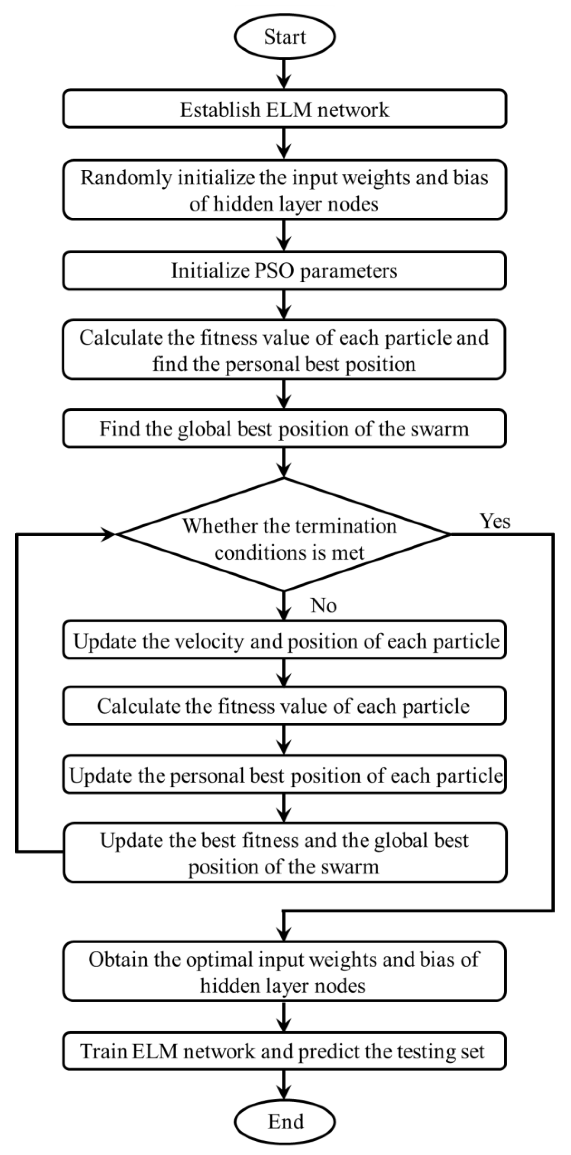
3.6. PSO-ELM Algorithm

As mentioned above, the input weights and bias of HLNs in the ELM algorithm are randomly generated. So, there may be some input weight matrices and bias of HLNs that are 0—that is, some HLNs are invalid [59]. This will reduce the accuracy of the prediction. In order to overcome this shortcoming, this paper combines PSO and ELM, called PSO-ELM. It uses the PSO algorithm to adjust the input weight matrices and bias of HLNs in ELM to make them better and then obtain an optimal network [59]. The flow of the PSO-ELM algorithm is shown in Figure 6.

4. Experimental Study

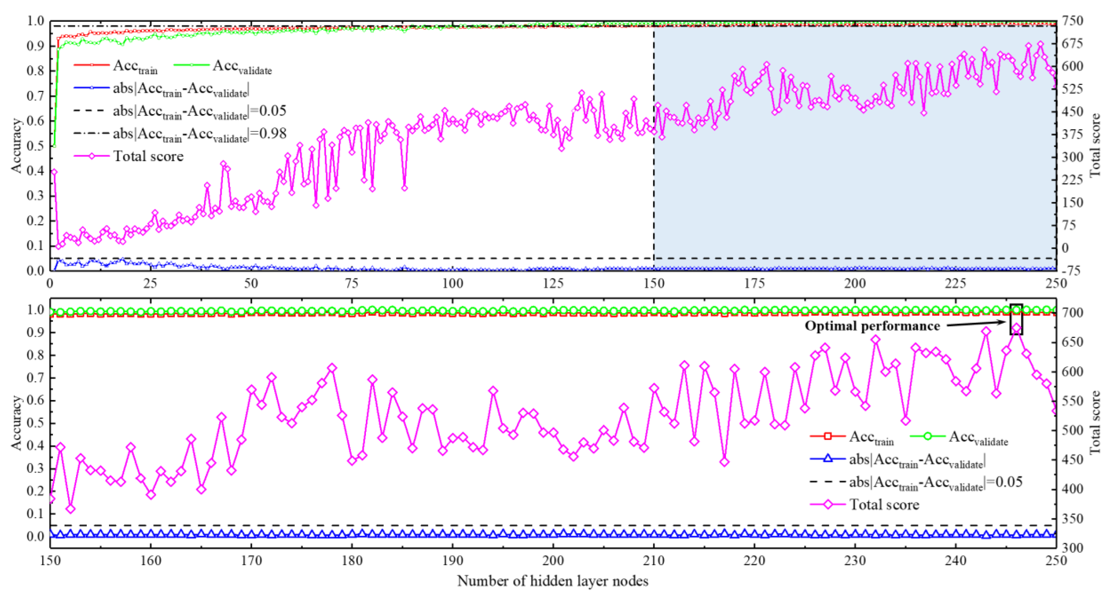
4.1. Development of the BPNN Model

The artificial neural network (ANN) with only one hidden layer can estimate almost all problems [61]. So, a single hidden layer BPNN was adopted in this paper. For the ANN architecture, NumHLNs is very important, and the determination of it is widely regarded as the most critical task. Caudill pointed out in his research that the upper limit of NumHLNs is 2 n + 1, where n denotes the number of input layer nodes [62]. So, 37 BPNN models with NumHLNs from 1 to 37 were developed according to n equals 18 in this paper. To avoid overfitting, the training set was randomly split into the training subset and the validation subset, which account for 75% and 25% of the training set, respectively. Then, the above 37 BPNN models were used to predict the training subset and the validation subset, and each was run 5 times (see Figure 7), which is also helpful to avoiding overfitting. Acctrain and Accvalidate in Figure 7 represent the average overall accuracy of each model predicting the training subset and the validation subset, respectively. The same is true in other figures.
The phenomenon that the prediction performance of the training subset significantly exceeds that of the validation subset is usually considered as the overfitting phenomenon; otherwise, it is called the underfitting phenomenon. Both overfitting and underfitting indicate that the model is unreliable. The prediction performance in Figure 7 shows that the differences between Acctrain and Accvalidate in the 37 BPNN models are all less than 5%, and the values of Acctrain and Accvalidate do not change much after NumHLNs exceeds 3. To find the optimally performing BPNN model among these 37 models, a ranking method proposed by Zorlu et al. [63] was adopted in this paper. Firstly, the Acctrain, Accvalidate and their difference abs|Acctrain−Accvalidate| of the 37 BPNN models were sorted from smallest to largest, respectively. Then, these three parameters were scored, and the model with the smallest Acctrain received 1 point, and the second smallest one received 2 points. In this order, the model with the largest Acctrain received 37 points. For Accvalidate, the models were also scored according to this rule. However, for abs|Acctrain−Accvalidate|, the opposite is true. The model with the smallest abs|Acctrain−Accvalidate| received 37 points and the largest one received 1 point. Finally, the three scores of each model were summed, and the model with the highest total score is optimal. It is obvious in Figure 7 that the model with 25 HLNs achieves the optimal performance, whose average Acctrain and average Accvalidate are 0.9577 and 0.9388, respectively. So, 25 was chosen as NumHLNs.

4.2. Development of the NBC Model

The development of the NBC model is relatively simple, because the parameters required for discrimination, including the mean and variance of each attribute and the prior probability of each class, only need to be estimated based on the training data. So, the NBC model was established after calculating the parameters required for discrimination based on the training set in this paper.

4.3. Development of the FDA Model

Similarly to the NBC model, the development process of the FDA model was relatively simple, and almost all parameters were calculated based on the training data. It should be noted that the threshold was calculated by multiplying the sum of the Fisher scores of the microseismic event and the blast by 0.5.

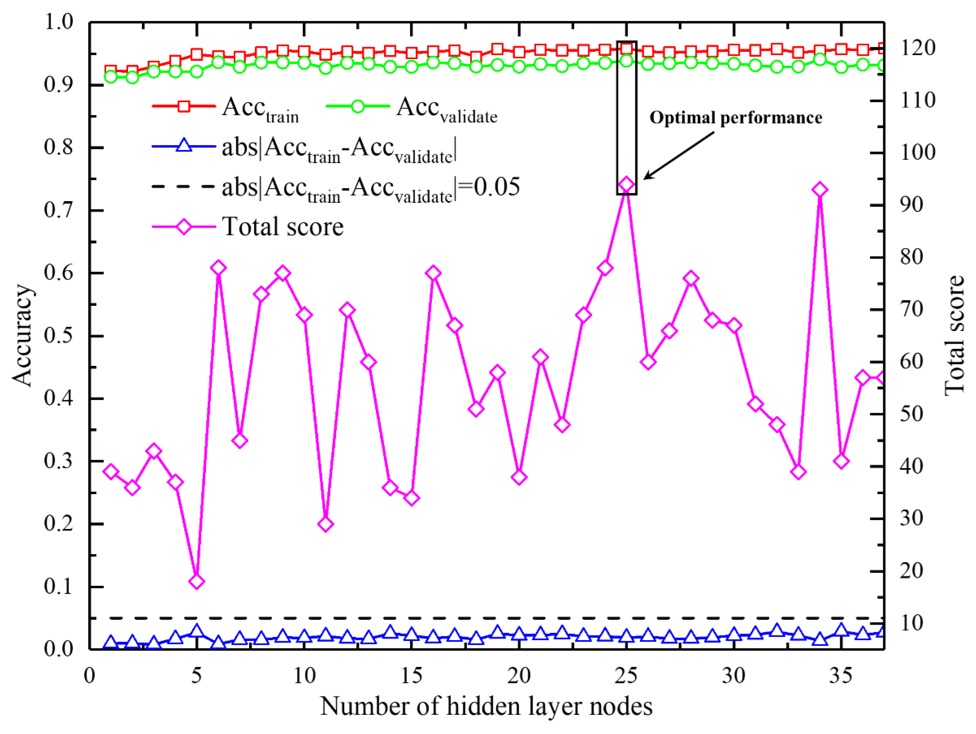
4.4. Development of the ELM Model

NumHLNs is related to whether ELM can achieve the expected prediction performance, and so it is necessary to investigate NumHLNs first to develop an optimal model. Two hundred ELM models with NumHLNs from 1 to 200 were developed, and each was run five times to predict the training subset and the validation subset (see Figure 8). As shown in Figure 8, 71 was chosen as NumHLNs after both considering the model performance and the thresholds of 5% between the overfitting and underfitting phenomenon, with an average Acctrain of 0.9425 and an average Accvalidate of 0.9238.

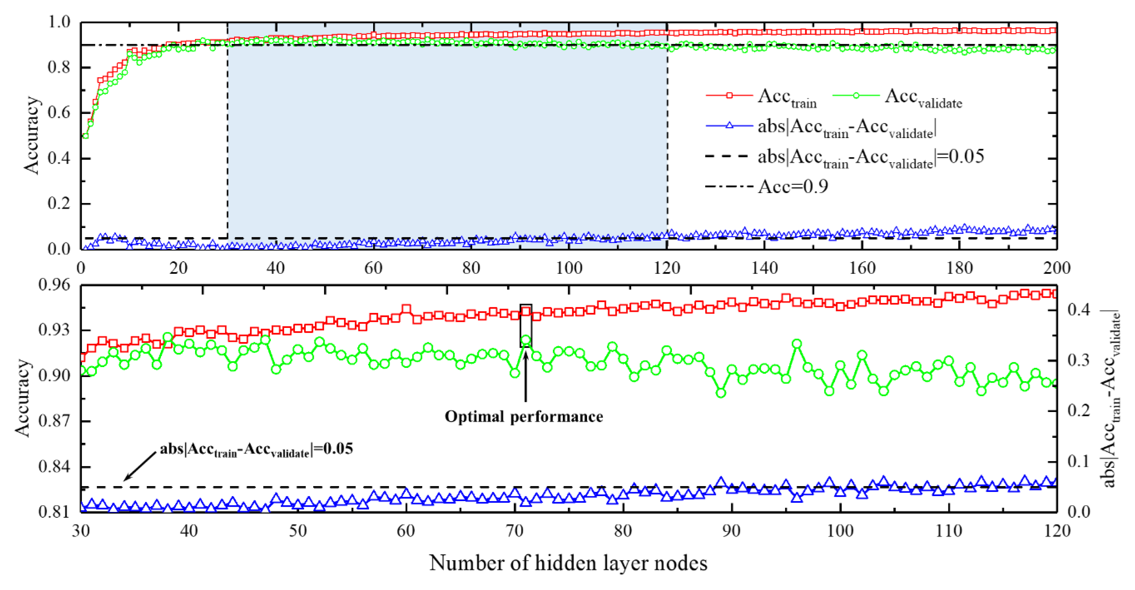
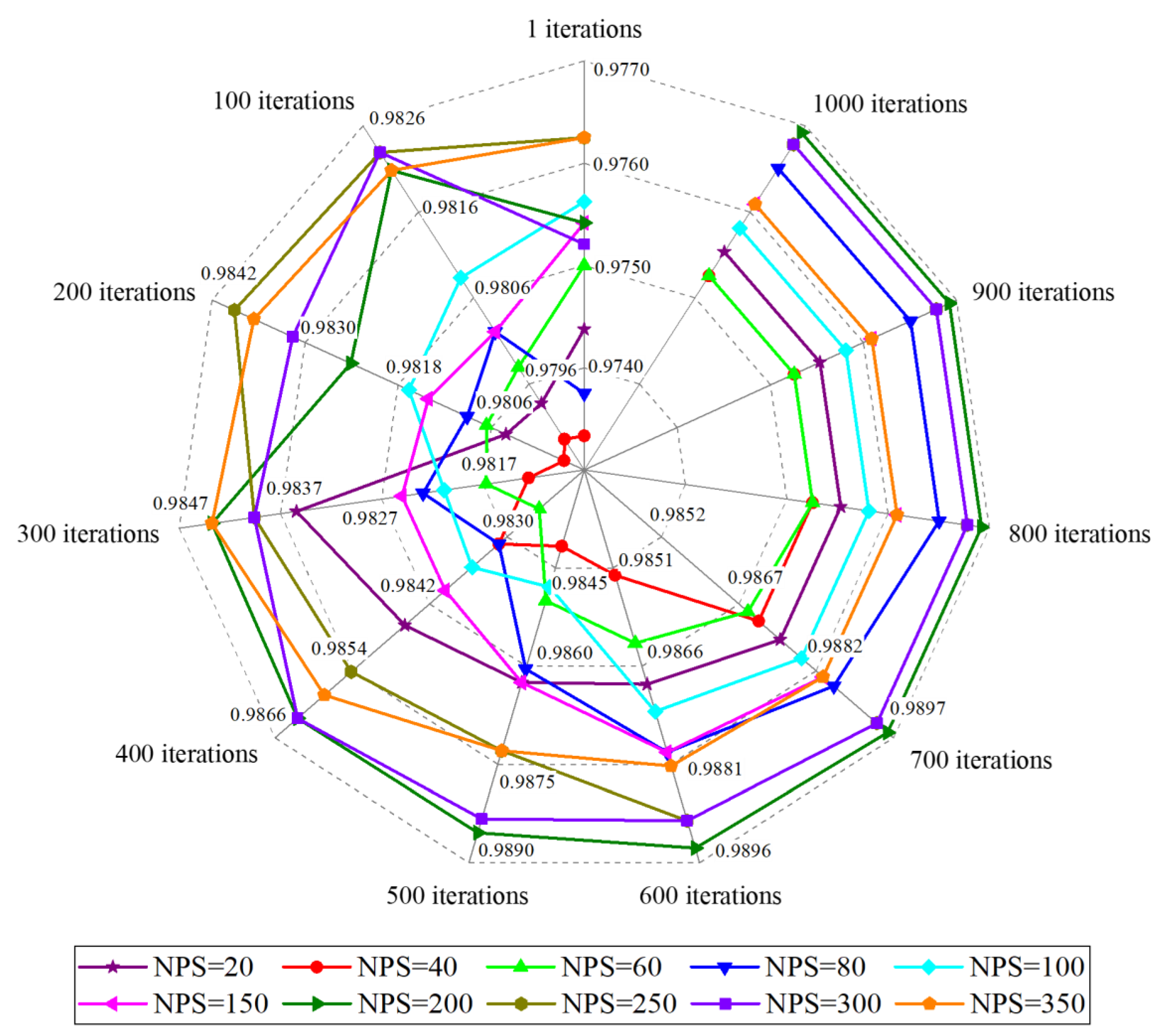
4.5. Development of PSO-ELM Model

Similarly to ELM, NumHLNs of PSO-ELM also needs to be investigated. So, 250 PSO-ELM models with NumHLNs from 1 to 250, with a number of particles in the swarm of 250 and a maximum iteration of 1000, were developed. Then, each model was run five times to predict the training subset and the validation subset (see Figure 9). The reason why models with more than 250 HLNs were not developed is that the computational load of the model increases sharply as NumHLNs increases. The prediction performance in Figure 9 shows that differences between Acctrain and Accvalidate in the 250 PSO-ELM models are all less than 5%, and when NumHLNs exceeds 100, the values of Acctrain and Accvalidate do not change much. To find the optimally performing PSO-ELM model among these 250 models, the ranking method presented by Zorlu et al. [63] was again adopted. It is obvious in Figure 9 that the model with 246 HLNs achieves the optimal performance, whose average Acctrain and average Accvalidate are 0.9915 and 0.9994, respectively. So, 246 was chosen as NumHLNs.
After NumHLNs in PSO-ELM was determined, the number of particles in the swarm (NPS) and the maximum number of iterations also need to be investigated. Hence, 10 PSO-ELM models with the maximum number of iterations of 1000 and the number of particles from 20 to 350 were established and run five times to predict the training subset (see Figure 10). As shown in Figure 10, there are no significant changes in these accuracy curves after 800 iterations, and 200 is the optimal NPS with the highest prediction accuracy. Thus, 800 and 200 were chosen to establish the final PSO-ELM model for discriminating microseismic events and mine blasts.

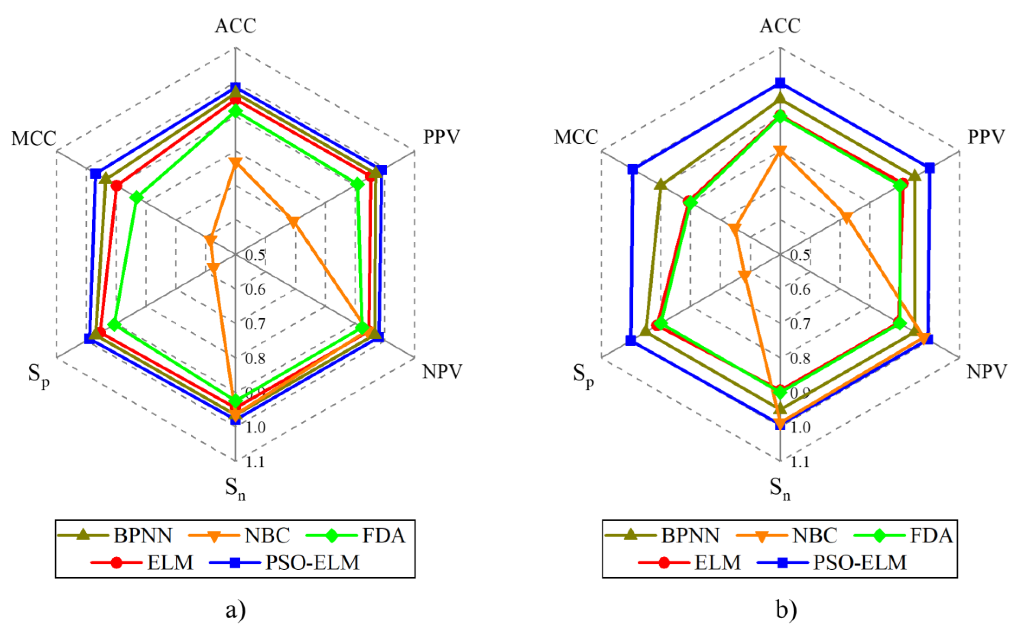
4.6. Quality Measures

To evaluate the performance of the discrimination models, six indicators were calculated, including the accuracy of the prediction ( A C C ), predictive positive value ( P P V ), negative predictive value ( N P V ), sensitivity ( S n ), specificity ( S p ) and Matthew’s correlation coefficient ( M C C ). The classification confusion matrix used to explain the above indicators is shown in Table 1, and microseismic events were assigned as positive, while blasts were assigned as negative.
These six indicators are defined as follows:
A C C = T P + T N T P + F N + F P + T N
P P V = T P T P + F P
N P V = T N T N + F N
S n = T P T P + F N
S p = T N T N + F P
M C C = T P × T N F P × F N ( T P + F P ) ( T P + F N ) ( T N + F P ) ( T N + F N )
A C C represents the overall prediction accuracy, which reflects the overall discrimination performance. P P V can be understood as the proportion of examples that are truly positive among all examples that are predicted to be positive. N P V can be understood as the proportion of examples that are truly negative among all examples that are predicted to be negative. S n can be understood as the proportion of examples predicted to be positive among all the true positive examples. S p can be understood as the proportion of examples predicted to be negative among all the true negative examples. These four indicators reflect the discrimination performance of positive and negative examples. M C C belongs to the index describing the relationship between the observation and prediction in binary classification problems which can evaluate the reliability of the algorithm [1]. Its value is between −1 and 1, where 1 indicates that the prediction performance is perfect, 0 indicates that the prediction performance is worse than that of random prediction, and −1 indicates that prediction totally disagrees with the observation [64]. Obviously, the higher the values of these six indicators, the better the discrimination performance of the model.

5. Results and Discussions

Based on the above investigation of optimal model parameters, the optimal models of five intelligent algorithms were established and used to predict the testing set after being trained by the training set. The discrimination results are shown in Table 2 and Figure 11. To better show the discrimination performance of the five models, a ranking method proposed by Zorlu et al. [63] was adopted in this paper. Firstly, each quality measuring indicator of the five models was sorted from smallest to largest. Then, they were scored, and the model with the smallest indicator value received 1 point, and the model with the second smallest indicator value received 2 points. In this order, the model with the largest indicator value received 5 points. Finally, the scores of the above six indicators of each model are summed, and the higher the total score, the better the discrimination performance. As shown in Table 2, the total score of PSO-ELM is the highest, followed by BPNN, ELM, FDA, and NBC. This shows that the discrimination performance of PSO-ELM is the best, followed by BPNN, ELM, FDA, and NBC. The values of the six indicators of PSO-ELM above are the highest, close to or equal to 1, which is almost perfect. This shows that PSO-ELM has an excellent performance in discriminating microseismic events and mine blasts.
Although some achievements have been obtained in this research, there are still some limitations. First of all, only the PSO-ELM algorithm was discussed and there are other intelligent algorithms that need to be tested for discriminating microseismic events and mine blasts. Secondly, in addition to these 22 seismic parameters, the impact of other seismic parameters on the performance of discrimination remains to be investigated. Finally, since the data of only one mine were used to check the performance of PSO-ELM, its universality is not yet clear.

6. Conclusions

Based on the differences between microseismic events and mine blasts, and combined with previous research conclusions, a new discrimination method for microseismic events and blasts is presented in this paper. In this method, 22 seismic parameters were selected as the discrimination feature parameters, and their correlation was analyzed. Then, the artificial intelligence model called PSO-ELM was used to discriminate microseismic events and mine blasts. After the development of the optimal model, this method was applied to the discrimination of microseismic records in Fankou Lead-Zinc Mine and compared with the original ELM and commonly used BPNN, NBC, and FDA to check its performance. The results show that PSO-ELM has the best discrimination performance regarding microseismic events and mine blasts, followed by BPNN, ELM, FDA, and NBC. In addition, the values of all quality measuring indicators of PSO-ELM are the highest. Specifically, the A C C , P P V , N P V , S n , S p and M C C of PSO-ELM predicting the training set are 0.9844, 0.9890, 0.9799, 0.9797, 0.9891 and 0.9688, respectively. The A C C , P P V , N P V , S n , S p and M C C of PSO-ELM predicting the testing set are 0.9969, 1, 0.9938, 0.9938, 1 and 0.9938, respectively. The values of these indicators are close to or equal to 1, which is almost perfect and shows that PSO-ELM has outstanding performance. In summary, PSO-ELM has great potential for the discrimination of microseismic events and blasts, and it is of great significance to ensure the safe and smooth operation of mines.

Author Contributions

Conceptualization, J.Z. (Jian Zhou); Investigation, D.R., Z.D. and J.Z. (Jinzhong Zhang); Methodology, D.R. and J.Z. (Jian Zhou); Project administration, X.S. and Y.G.; Software, D.R.; Supervision, X.S. and Z.Y.; Visualization, D.R.; Writing—original draft, D.R.; Writing—review & editing, Z.Y. and Y.G. All authors have read and agreed to the published version of the manuscript.

Funding

The National Natural Science Foundation Project of China (Grant No. 51874350, Xiuzhi Shi). The National Natural Science Foundation Project of China (Grant No. 41807259, A.P. Jian Zhou). The National Key R&D Program of China (2017YFC0602902, Prof. Xiuzhi Shi). The Fundamental Research Funds for the Central Universities of Central South University (2020zzts200, Dijun Rao). The Innovation-Driven Project of Central South University (2020CX040, A.P. Jian Zhou).

Institutional Review Board Statement

Not applicable.

Informed Consent Statement

Not applicable.

Data Availability Statement

Not applicable.

Acknowledgments

The authors acknowledge the financial support from the National Natural Science Foundation Project of China (Grant No. 51874350 and 41807259), the Fundamental Research Funds for the Central Universities of Central South University (2020zzts200), the National Key R&D Program of China (2017YFC0602902), and the Innovation-Driven Project of Central South University (2020CX040) for carrying out this research work. The authors thank Fankou Lead-Zinc Mine and Shanghai PengXu Information and Technology Co., Ltd. for their full support and Xueyi Shang of Chongqing University for his help.

Conflicts of Interest

The authors declare no conflict of interest.

References

  1. Zhang, J.Y.; Jiang, R.C.; Li, B.; Xu, N.W. An automatic recognition method of microseismic signals based on EEMD-SVD and ELM. Comput. Geosci. 2019, 133. [Google Scholar] [CrossRef]
  2. Liu, J.P.; Feng, X.T.; Li, Y.H.; Xu, S.D.; Sheng, Y. Studies on temporal and spatial variation of microseismic activities in a deep metal mine. Int. J. Rock Mech. Min. Sci. 2013, 60, 171–179. [Google Scholar] [CrossRef]
  3. Potvin, Y.; Hudyma, M.R. Seismic monitoring in highly mechanized hardrock mines in Canada and Australia. In Proceedings of the 5th International Symposium on Rockburst and Seismicity in Mines Proceedings, Johannesbury, South Africa, 1 January 2001; pp. 1–22. [Google Scholar]
  4. Li, B.; Li, T.; Xu, N.W.; Dai, F.; Chen, W.F.; Tan, Y.S. Stability assessment of the left bank slope of the Baihetan Hydropower Station, Southwest China. Int. J. Rock Mech. Min. Sci. 2018, 104, 34–44. [Google Scholar] [CrossRef]
  5. Dai, F.; Jiang, P.; Xu, N.W.; Chen, W.F.; Tan, Y.S. Focal mechanism determination for microseismic events and its application to the left bank slope of the Baihetan hydropower station in China. Environ. Earth Sci. 2018, 77, 1–15. [Google Scholar] [CrossRef]
  6. Xu, N.W.; Li, T.B.; Dai, F.; Li, B.; Zhu, Y.G.; Yang, D.S. Microseismic monitoring and stability evaluation for the large scale underground caverns at the Houziyan hydropower station in Southwest China. Eng. Geol. 2015, 188, 48–67. [Google Scholar] [CrossRef]
  7. Dai, F.; Li, B.; Xu, N.W.; Fan, Y.L.; Zhang, C.Q. Deformation forecasting and stability analysis of large-scale underground powerhouse caverns from microseismic monitoring. Int. J. Rock Mech. Min. Sci. 2016, 86, 269–281. [Google Scholar] [CrossRef]
  8. Feng, X.T.; Chen, B.R.; Li, S.J.; Zhang, C.Q.; Xiao, Y.X.; Feng, G.L.; Zhou, H.; Qiu, S.L.; Zhao, Z.N.; Yu, Y.; et al. Studies on the evolution process of rockbursts in deep tunnels. J. Rock Mech. Geotech. Eng. 2012, 4, 289–295. [Google Scholar] [CrossRef]
  9. Ma, T.H.; Tang, C.A.; Tang, L.X.; Zhang, W.D.; Wang, L. Rockburst characteristics and microseismic monitoring of deep-buried tunnels for Jinping II Hydropower Station. Tunn. Undergr. Space Technol. 2015, 49, 345–368. [Google Scholar] [CrossRef]
  10. Bi, L.; Xie, W.; Zhao, J.J. Automatic recognition and classification of multi-channel microseismic waveform based on DCNN and SVM. Comput. Geosci. 2019, 123, 111–120. [Google Scholar] [CrossRef]
  11. Xiao, Y.X.; Feng, X.T.; Hudson, J.A.; Chen, B.R.; Feng, G.L.; Liu, J.P. ISRM Suggested Method for In Situ Microseismic Monitoring of the Fracturing Process in Rock Masses. Rock Mech. Rock Eng. 2016, 49, 343–369. [Google Scholar] [CrossRef]
  12. Dong, L.J.; Wesseloo, J.; Potvin, Y.; Li, X.B. Discriminant models of blasts and seismic events in mine seismology. Int. J. Rock Mech. Min. Sci. 2016, 86, 282–291. [Google Scholar] [CrossRef]
  13. Shang, X.Y.; Li, X.B.; Morales-Esteban, A.; Chen, G.H. Improving microseismic event and quarry blast classification using Artificial Neural Networks based on Principal Component Analysis. Soil Dyn. Earthq. Eng. 2017, 99, 142–149. [Google Scholar] [CrossRef]
  14. Derr, J.S. Discrimination of earthquakes and explosions by the Rayleigh- wave spectral ratio. Bull. Seismol. Soc. Am. 1970, 60, 1653–1668. [Google Scholar]
  15. Zeiler, C.; Velasco, A.A. Developing local to near-regional explosion and earthquake discriminants. Bull. Seismol. Soc. Am. 2009, 99, 24–35. [Google Scholar] [CrossRef]
  16. Kim, W.Y.; Aharonian, V.; Lerner-Lam, A.L.; Richards, P.G. Discrimination of earthquakes and explosions in Southern Russia using regional high-frequency three-component data from the IRIS/JSP Caucasus Network. Bull. Seismol. Soc. Am. 1997, 87, 569–588. [Google Scholar]
  17. Ford, S.R.; Walter, W.R. Aftershock characteristics as a means of discriminating explosions from earthquakes. Bull. Seismol. Soc. Am. 2010, 100, 364–376. [Google Scholar] [CrossRef]
  18. Yu, Z.; Shi, X.Z.; Zhou, J.; Rao, D.J.; Chen, X.; Dong, W.M.; Miao, X.H.; Ipangelwa, T. Feasibility of the indirect determination of blast-induced rock movement based on three new hybrid intelligent models. Eng. Comput. 2019. [Google Scholar] [CrossRef]
  19. Yu, Z.; Shi, X.Z.; Qiu, X.Y.; Zhou, J.; Chen, X.; Gou, Y.G. Optimization of postblast ore boundary determination using a novel sine cosine algorithm-based random forest technique and Monte Carlo simulation. Eng. Optim. 2020, 1–16. [Google Scholar] [CrossRef]
  20. Zhou, J.; Li, X.B.; Shi, X.Z. Long-term prediction model of rockburst in underground openings using heuristic algorithms and support vector machines. Saf. Sci. 2012, 50, 629–644. [Google Scholar] [CrossRef]
  21. Nguyen, H.; Bui, X.N. Predicting Blast-Induced Air Overpressure: A Robust Artificial Intelligence System Based on Artificial Neural Networks and Random Forest. Nat. Resour. Res. 2019, 28, 893–907. [Google Scholar] [CrossRef]
  22. Yu, Z.; Shi, X.Z.; Chen, X.; Zhou, J.; Qi, C.C.; Chen, Q.S.; Rao, D.J. Artificial intelligence model for studying unconfined compressive performance of fiber-reinforced cemented paste backfill. Trans. Nonferrous Met. Soc. China 2021, 31, 1087–1102. [Google Scholar] [CrossRef]
  23. Kortström, J.; Uski, M.; Tiira, T. Automatic classification of seismic events within a regional seismograph network. Comput. Geosci. 2016, 87, 22–30. [Google Scholar] [CrossRef] [Green Version]
  24. Vallejos, J.A.; McKinnon, S.D. Logistic regression and neural network classification of seismic records. Int. J. Rock Mech. Min. Sci. 2013, 62, 86–95. [Google Scholar] [CrossRef]
  25. Bui Quang, P.; Gaillard, P.; Cano, Y.; Ulzibat, M. Detection and classification of seismic events with progressive multi-channel correlation and hidden Markov models. Comput. Geosci. 2015, 83, 110–119. [Google Scholar] [CrossRef]
  26. Malovichko, D. Discrimination of blasts in mine seismology. In Proceedings of the Sixth International Seminar on Deep and High Stress Mining, Perth, Australia, 23–30 March 2012; pp. 161–172. [Google Scholar] [CrossRef] [Green Version]
  27. Zhao, G.Y.; Ma, J.; Dong, L.J.; Li, X.B.; Chen, G.H.; Zhang, C.X. Classification of mine blasts and microseismic events using starting-up features in seismograms. Trans. Nonferrous Met. Soc. China 2015, 25, 3410–3420. [Google Scholar] [CrossRef]
  28. Dong, L.; Li, X.; Xie, G. Nonlinear methodologies for identifying seismic event and nuclear explosion using random forest, support vector machine, and naive bayes classification. Abstr. Appl. Anal. 2014, 2014. [Google Scholar] [CrossRef] [Green Version]
  29. Mendecki, A.J. Seismic Monitoring in Mines. Seism. Monit. Mines 1996. [Google Scholar] [CrossRef]
  30. Ma, J.; Zhao, G.Y.; Dong, L.J.; Chen, G.H.; Zhang, C.X. A comparison of mine seismic discriminators based on features of source parameters to waveform characteristics. Shock Vib. 2015, 2015. [Google Scholar] [CrossRef] [Green Version]
  31. Chen, X.; Shi, X.Z.; Zhou, J.; Li, E.M.; Qiu, P.Y.; Gou, Y.G. High strain rate compressive strength behavior of cemented paste backfill using split Hopkinson pressure bar. Int. J. Min. Sci. Technol. 2021, 31, 387–399. [Google Scholar] [CrossRef]
  32. Chen, Q.S.; Sun, S.Y.; Qi, C.C.; Liu, Y.K.; Zhou, H.B.; Zhang, Q.L. Experimental and numerical study on immobilization and leaching characteristics of fluoride from phosphogypsum based cemented paste backfill. Int. J. Miner. Metall. Mater. 2021, 28. [Google Scholar] [CrossRef]
  33. Bormann, P. New Manual of Seismological Observatory Practice (NMSOP); GeoForschungs Zentrum Potsdam: Potsdam, Germany, 2002. [Google Scholar]
  34. Rovini, E.; Maremmani, C.; Moschetti, A.; Esposito, D.; Cavallo, F. Comparative Motor Pre-clinical Assessment in Parkinson’s Disease Using Supervised Machine Learning Approaches. Ann. Biomed. Eng. 2018, 46, 2057–2068. [Google Scholar] [CrossRef]
  35. Adoko, A.C.; Gokceoglu, C.; Wu, L.; Zuo, Q.J. Knowledge-based and data-driven fuzzy modeling for rockburst prediction. Int. J. Rock Mech. Min. Sci. 2013, 61, 86–95. [Google Scholar] [CrossRef]
  36. Zhou, J.; Koopialipoor, M.; Li, E.M.; Armaghani, D.J. Prediction of rockburst risk in underground projects developing a neuro-bee intelligent system. Bull. Eng. Geol. Environ. 2020. [Google Scholar] [CrossRef]
  37. Xu, C.; Gordan, B.; Koopialipoor, M.; Armaghani, D.J.; Tahir, M.M.; Zhang, X. Improving Performance of Retaining Walls under Dynamic Conditions Developing an Optimized ANN Based on Ant Colony Optimization Technique. IEEE Access 2019, 7, 94692–94700. [Google Scholar] [CrossRef]
  38. Wu, X.; Sun, C.; Zou, T.; Xiao, H.; Wang, L.; Zhai, J. Intelligent path recognition against image noises for vision guidance of automated guided vehicles in a complex workspace. Appl. Sci. 2019, 9, 4108. [Google Scholar] [CrossRef] [Green Version]
  39. Wang, J.; Zhang, X.; Guo, Z.; Lu, H. Developing an early-warning system for air quality prediction and assessment of cities in China. Expert Syst. Appl. 2017, 84, 102–116. [Google Scholar] [CrossRef]
  40. Li, C.Q.; Zhou, J.; Jahed-Armaghani, D.; Li, X.B. Stability analysis of underground mine hard rock pillars via combination of finite difference methods, neural networks, and Monte Carlo simulation techniques. Undergr. Space 2020. [Google Scholar] [CrossRef]
  41. Abraham, R.; Simha, J.B.; Iyengar, S.S. A comparative analysis of discretization methods for medical datamining with Naïve Bayesian classifier. In Proceedings of the 9th International Conference on Information Technology, ICIT 2006, Bhubaneswar, India, 18–21 December 2006; pp. 235–236. [Google Scholar]
  42. Boyles, S.; Fajardo, D.; Waller, S.T. Naive bayesian classifier for incident duration prediction. In Proceedings of the Transportation Research Board 86th Annual Meeting, Washington, DC, USA, 21–25 December 2007; p. 253. [Google Scholar]
  43. Domingos, P.; Pazzani, M. On the Optimality of the Simple Bayesian Classifier underZero-One Loss. Mach. Learn. 1997, 29, 103–130. [Google Scholar] [CrossRef]
  44. Ratanamahatana, C.; Gunopulos, D. Feature selection for the naive bayesian classifier using decision trees. Appl. Artif. Intell. 2003, 17, 475–487. [Google Scholar] [CrossRef]
  45. Li, B.; Li, H. Prediction of tunnel face stability using a naive Bayes classifier. Appl. Sci. 2019, 9, 4319. [Google Scholar] [CrossRef] [Green Version]
  46. Zhou, J.; Li, X.B.; Mitri, H.S. Classification of rockburst in underground projects: Comparison of ten supervised learning methods. J. Comput. Civ. Eng. 2016, 30. [Google Scholar] [CrossRef]
  47. Jiang, C.L.; Jiang, Z.Q.; Sun, Q. Classification of rocks surrounding tunnel using Fisher discriminant analysis method. Meitan Xuebao/J. China Coal Soc. 2012, 37, 1665–1670. [Google Scholar] [CrossRef]
  48. AbuZeina, D.; Al-Anzi, F.S. Employing fisher discriminant analysis for Arabic text classification. Comput. Electr. Eng. 2018, 66, 474–486. [Google Scholar] [CrossRef]
  49. Zhong, S.; Wen, Q.; Ge, Z. Semi-supervised Fisher discriminant analysis model for fault classification in industrial processes. Chemom. Intell. Lab. Syst. 2014, 138, 203–211. [Google Scholar] [CrossRef]
  50. Yu, J. Nonlinear bioprocess monitoring using multiway kernel localized fisher discriminant analysis. Ind. Eng. Chem. Res. 2011, 50, 3390–3402. [Google Scholar] [CrossRef]
  51. Zhou, J.; Li, X.B.; Shi, X.Z.; Wei, W.; Wu, B.B. Predicting pillar stability for underground mine using Fisher discriminant analysis and SVM methods. Trans. Nonferrous Met. Soc. China 2011, 21, 2734–2743. [Google Scholar] [CrossRef]
  52. Huang, G.B.; Zhu, Q.Y.; Siew, C.K. Extreme learning machine: Theory and applications. Neurocomputing 2006, 70, 489–501. [Google Scholar] [CrossRef]
  53. Zhang, J.; Xiao, W.; Li, Y.; Zhang, S.; Zhang, Z. Multilayer probability extreme learning machine for device-free localization. Neurocomputing 2020, 396, 383–393. [Google Scholar] [CrossRef]
  54. Figueiredo, E.M.N.; Ludermir, T.B. Investigating the use of alternative topologies on performance of the PSO-ELM. Neurocomputing 2014, 127, 4–12. [Google Scholar] [CrossRef]
  55. Eberhart, R.; Kennedy, J. A New Optimizer Using Particle Swarm Theory. In Proceedings of the Sixth International Symposium on Micro Machine and Human Science, Nagoya, Japan, 4–6 October 1995. [Google Scholar]
  56. Armaghani, D.J.; Koopialipoor, M.; Marto, A.; Yagiz, S. Application of several optimization techniques for estimating TBM advance rate in granitic rocks. J. Rock Mech. Geotech. Eng. 2019, 11, 779–789. [Google Scholar] [CrossRef]
  57. Koopialipoor, M.; Jahed-Armaghani, D.; Hedayat, A.; Marto, A.; Gordan, B. Applying various hybrid intelligent systems to evaluate and predict slope stability under static and dynamic conditions. Soft Comput. 2019, 23, 5913–5929. [Google Scholar] [CrossRef]
  58. Hasanipanah, M.; Naderi, R.; Kashir, J.; Noorani, S.A.; Zeynali-Aaq-Qaleh, A. Prediction of blast-produced ground vibration using particle swarm optimization. Eng. Comput. 2017, 33, 173–179. [Google Scholar] [CrossRef]
  59. Cai, W.H.; Yang, J.J.; Yu, Y.D.; Song, Y.Y.; Zhou, T.; Qin, J. PSO-ELM: A Hybrid Learning Model for Short-Term Traffic Flow Forecasting. IEEE Access 2020, 8, 6505–6514. [Google Scholar] [CrossRef]
  60. Yuhui, S.; Eberhart, R. A modified particle swarm optimizer. In Proceedings of the IEEE International Conference on IEEE World Congress on Computational Intelligence, Anchorage, AK, USA, 4–9 May 1998; pp. 69–73. [Google Scholar]
  61. Hasanipanah, M.; Noorian-Bidgoli, M.; Jahed Armaghani, D.; Khamesi, H. Feasibility of PSO-ANN model for predicting surface settlement caused by tunneling. Eng. Comput. 2016, 32, 705–715. [Google Scholar] [CrossRef]
  62. Caudill, M. Neural Networks Primer Part III; Al Expert: Lawrence, KS, USA, 1988; pp. 53–59. [Google Scholar]
  63. Zorlu, K.; Gokceoglu, C.; Ocakoglu, F.; Nefeslioglu, H.A.; Acikalin, S. Prediction of uniaxial compressive strength of sandstones using petrography-based models. Eng. Geol. 2008, 96, 141–158. [Google Scholar] [CrossRef]
  64. Asencio-Cortés, G.; Martínez-Álvarez, F.; Troncoso, A.; Morales-Esteban, A. Medium–large earthquake magnitude prediction in Tokyo with artificial neural networks. Neural Comput. Appl. 2017, 28, 1043–1055. [Google Scholar] [CrossRef]
Figure 1. Fankou Lead-Zinc Mine. (a) Mine’s position in China; (b) a view of the mine; (c) mine’s position in Guangdong province.
Applsci 11 06474 g001
Figure 2. The IMS system in Fankou Lead-Zinc Mine.
Applsci 11 06474 g002
Figure 3. Violin plots of the distribution of the 22 seismic parameters in the sample dataset. The box in each plot indicates the lower ( Q 1 ) and upper ( Q 3 ) quartiles, and the red circle indicates the median value. The value of Q 3 minus Q 1 is defined as the interquartile range ( IQR ). The range of whiskers at both ends of the box represents the upper and lower bounds, which are defined as Q 3 + 1 . 5 IQR and Q 1 - 1 . 5 IQR , respectively. Cyan represents the distribution of data points.
Applsci 11 06474 g003
Figure 4. Heatmap of the correlation coefficients between 22 seismic parameters.
Applsci 11 06474 g004
Figure 5. ELM network structure.
Applsci 11 06474 g005
Figure 6. Flowchart of PSO-ELM Algorithm.
Applsci 11 06474 g006
Figure 7. Prediction results of the BPNN models with various HLNs.
Applsci 11 06474 g007
Figure 8. Prediction results of the ELM model with various HLNs.
Applsci 11 06474 g008
Figure 9. Prediction results of the PSO-ELM model with various HLNs.
Applsci 11 06474 g009
Figure 10. Accuracy curves of 10 PSO-ELM models with 1000 iterations and various NPS.
Applsci 11 06474 g010
Figure 11. Discrimination results for different discrimination models. (a) the training set; (b) the testing set.
Applsci 11 06474 g011
Table 1. A typical binary classification confusion matrix.
TruePredict
Positive ExampleNegative Example
Positive exampleTrue positive (TP)False negative (FN)
Negative exampleFalse positive (FP)True negative (TN)
Table 2. Discrimination results for different discrimination models.
ModelDatasetResultsScoreTotal Score
ACCPPVNPVSnSpMCCACCPPVNPVSnSpMCC
BPNNTraining0.96720.96870.96570.96560.96880.934444444446
Testing0.95000.95000.95000.95000.95000.9000443344
NBCTraining0.76880.69330.94100.96410.57340.583911231121
Testing0.80310.72150.98020.98750.61880.6522114411
FDATraining0.91560.90800.92360.92500.90630.831422112222
Testing0.90000.90000.90000.90000.90000.8000222222
ELMTraining0.94920.95280.94570.94530.95310.898533323331
Testing0.90310.91080.89570.89380.91250.8064331133
PSO-ELMTraining0.98440.98900.97990.97970.98910.968855555560
Testing0.99691.00000.99380.99381.00000.9938555555
Publisher’s Note: MDPI stays neutral with regard to jurisdictional claims in published maps and institutional affiliations.

