A Two-Phase Approach for Predicting Highway Passenger Volume

Abstract

With the continuous process of urbanization, regional integration has become an inevitable trend of future social development. Accurate prediction of passenger volume is an essential prerequisite for understanding the extent of regional integration, which is one of the most fundamental elements for the enhancement of intercity transportation systems. This study proposes a two-phase approach in an effort to predict highway passenger volume. The datasets subsume highway passenger volume and impact factors of urban attributes. In Phase I, correlation analysis is conducted to remove highly correlated impact factors, and a random forest algorithm is employed to extract significant impact factors based on the degree of impact on highway passenger volume. In Phase II, a deep feedforward neural network is developed to predict highway passenger volume, which proved to be more accurate than both the support vector machine and multiple regression methods. The findings can provide useful information for guiding highway planning and optimizing the allocation of transportation resources.

1. Introduction

Recently, with the continuous process of urbanization, regional integration has become an inevitable trend of future social development in many developing countries [1,2]. In this situation, establishing a convenient and efficient intercity transportation system is a prerequisite for supporting regional integration, in which accurate prediction of passenger volume is one of the most fundamental elements required for the enhancement of intercity transportation systems [3,4,5,6].

The primary concern of passenger volume prediction is to extract relevant impact factors and build appropriate models. Firstly, multiple impact factors related to urban attributes, such as gross domestic product (GDP) and population, determine the absolute value and spatial distribution of passenger volume [7,8]. Consequently, extracting significant impact factors and further analyzing their relationship with passenger volume is recognized as a prerequisite for accurately predicting the passenger volume. Secondly, the prediction models attracted wide attention and the performance of different models was evaluated in past research. Some typical models, including multiple logit models, machine learning models, and deep learning models have been developed based on the historical passenger volume [9,10]. Nevertheless, the predicted accuracy of the existing models was largely affected by the dataset size of historical passenger volume [11]. Hence, the models with historical data cannot perform an accurate prediction if lacking sufficient data, which is quite common for intercity transportation.

There are two key steps in the prediction of intercity passenger volume: (1) extracting the significant impact factors, (2) developing a deep learning model to achieve the prediction. Thus, it is practical to develop a two-phase approach to predicting intercity passenger volume based on impact factors reflecting urban attributes and deep learning models. As the highway is always an important intercity mode of transport with a high mode share, this study took the highway as the research object. Phase Ⅰ made a correlation analysis to remove the highly correlated impact factors and developed a random forest (RF) algorithm to extract the significant impact factors of highway passenger volume; Then, Phase Ⅱ developed a deep feedforward neural network (DFNN) to predict highway passenger volume. To overcome the existing limitations on predicting intercity passenger volume, the primary contributions of this study are as follows:

(1)

A total of 69 impact factors of urban attributes were collected from 280 administrative districts in China, which provides a macroscopic dataset for the prediction of highway passenger volume and overcomes the limitations of traditional travel surveys and questionnaires that only focus on a single city or single transportation corridor;

(2)

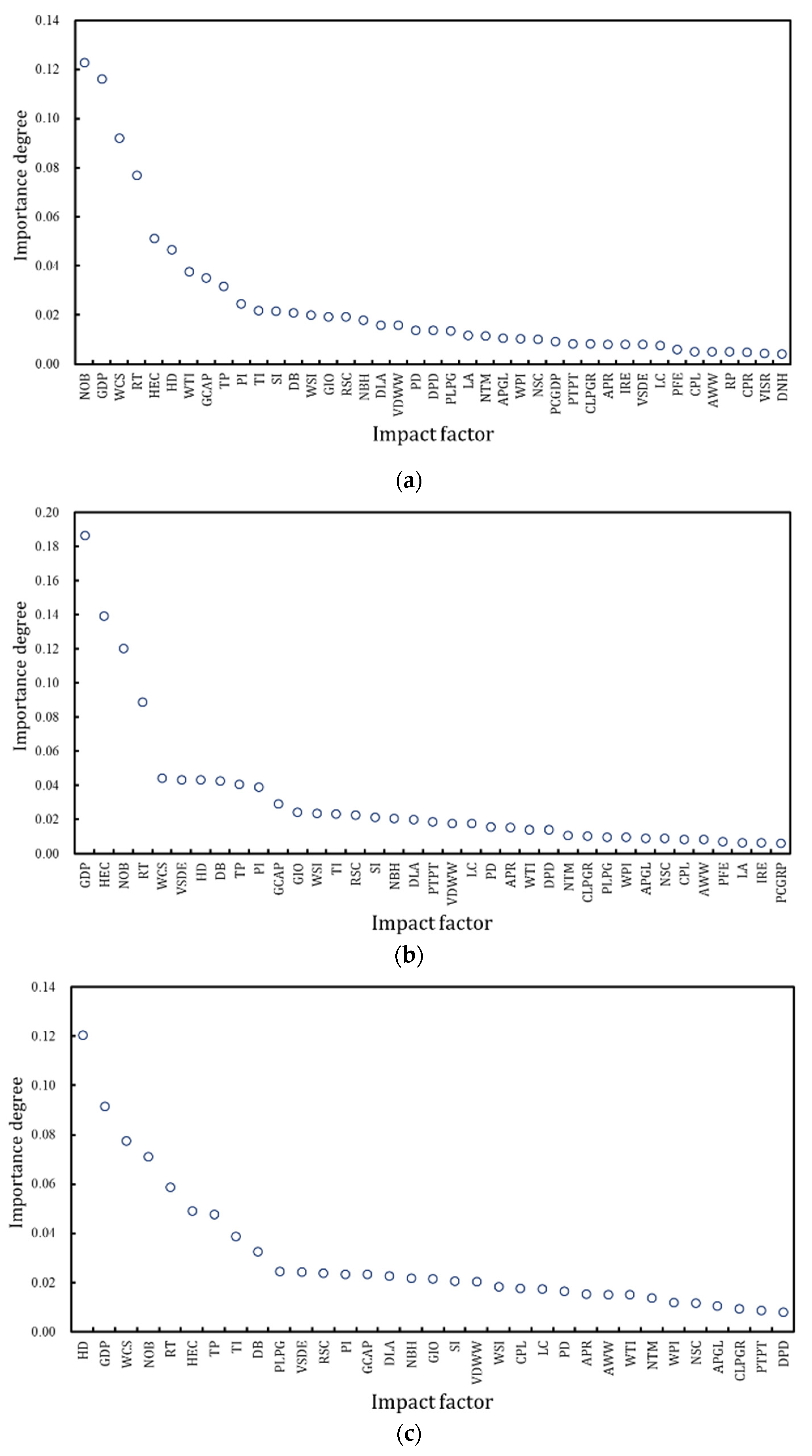
Multiple urban attributes, including urban economy, population, industry, income and consumption, and resource and environment, were modeled together. Furthermore, A total of 30 significant impact factors of highway passenger volume were extracted by the RF algorithm, which improves the traditional process based on subjective experience and avoids the omission of significant factors;

(3)

A deep learning method, DFNN, was developed to predict highway passenger volume, which proved to be more accurate than the SVM and multiple regression methods and can provide more reliable information for optimizing traffic structure and reducing waste of traffic resources.

The remainder of this study is organized as follows. Section 2 gives as overview of the related literature. In Section 3, the data source is introduced, and the impact factors of urban attributes are collected and presented. Section 4 presents the underlying principle of the RF and DFNN algorithm. Section 5 presents the process of extracting the significant impact factors. In Section 6, the DFNN is developed to predict highway passenger volume, which is further compared with two benchmark methods. Finally, Section 7 draws conclusions and gives an outlook on future research.

2. Literature Review

This section concludes the existing research on the above two phases: (1) extracting the significant impact factors of intercity passenger volume, (2) developing models to achieve an accurate prediction. Furthermore, the limitations of existing research are itemized at the end.

The first phase is to extract the significant impact factors. Multiple impact factors related to urban attributes, including urban economic level, urban industrial structure, population, etc., were widely studied to understand their relationship with intercity passenger volume. Firstly, the urban economic level proved to be one of the necessary impact factors of intercity passenger volume [12,13,14]. Traffic demand for business and tourism in intercity transportation increases with the development of the urban economy. The impact factors reflecting the urban economic level were found to be per-capita gross domestic product (GDP), per-capita income, industrial structure, etc., and it was verified that they had a strong correlation with intercity passenger volume [15,16]. Moreover, both population structure and population size affect the intercity passenger volume significantly. Limtanakool et al. [17] took population density and land use as variables and found that a higher population density and mixed degree of land use have a positive impact on passenger volume of public modes in medium- and long-distance trips. A similar conclusion was also reached by related research [18]. Although the impact factors related to economic level and population have been widely studied in the existing research, those related to the quality of residents’ lives, resources, and the environment were rarely studied because they are hard to be quantified with one or several indicators and the corresponding dataset is difficult to obtain [19,20,21]. This problem indicates that the relative research on extracting significant impact factors of intercity passenger volume is incomplete and causes the inaccurate prediction of intercity passenger volume, especially for some tourism-driven cities and resource-driven cities.

The second phase is to develop a model to achieve an accurate prediction of intercity passenger volume. In the existing studies, multiple logit models, such as the multinomial logit model [22,23], Box–Cox logit model [24], and nested logit model [25], were developed to study the mode choice of intercity trips and deduce the intercity passenger volume of various modes by calculating the intercity travel rate of surveyed samples [26,27]. Moreover, intercity passenger volume was predicted by introducing the impact factors. Harker et al. [28] proposed a network equilibrium model with considerations of market price and economic mechanism to predict the intercity freight volume. Li et al. [29] predicted the passenger volume of intercity railway with multiple indicators of passenger demand, regional economy, and regional traffic infrastructure, with an average predicted error of 3.37%. Another practical approach to predicting intercity passenger volume is based on the historical passenger volume. Xie et al. [30] analyzed the spatiotemporal characteristics of intercity passenger volume and predicted intercity passenger volume on holiday, with a predicted error of 6.43%. Recently, deep learning and machine learning algorithms, represented by various neural networks, have become remarkable at predicting intercity passenger volume by using cellular signaling data and location-based data [4,22,23,24,25,26,27,28,29,30,31,32]. Numerous studies have shown that predicted accuracy can be significantly improved by deep learning algorithms [33].

It is noted that the difficulties in obtaining the dataset of intercity passenger volume have been widely emphasized in past studies, especially for some intercity passenger modes of transportation that have additional requirements for an urban population, geographical location, or urban scale, such as airways, railways, and waterways. This means that the prediction of intercity passenger volume can be only conducted in a few cities [34]. In contrast, the highway has better accessibility and connects to all kinds of cities, expanding the study scope of predicting intercity passenger volume [35]. As previously stated, intercity passenger volume is largely determined by impact factors. Thus, the process of extracting significant impact factors at first, and then analyzing the interaction between intercity passenger volume and impact factors with deep learning algorithms, is practical for predicting intercity passenger volume but has rarely been studied in the existing research.

From the above analysis, the relationship between intercity passenger volume and urban attributes has been widely studied, and some typical models have been developed to predict passenger volume. Nevertheless, some limitations still exist in previous research and need further improvement, which are listed as follows:

(1)

Due to the restrictions of the research data, most existing research predicted intercity passenger volume from a single city or transportation corridor. As a result, the current achievements are difficult to apply to intercity transportation between all kinds of cities.

(2)

Existing research only focuses on common urban attributes such as the population or the economy. However, more urban attributes related to the quality of residents’ lives, resources, and environment were neglected for lacking the available data and quantitative indicators, causing the inaccurate prediction of intercity passenger volume, especially in some tourism-driven cities and resource-driven cities. Moreover, the selection process of significant attributes also received less attention.

(3)

Microcosmic datasets collected from traffic surveys have been widely used for studying the choice of transportation mode in intercity trips but is not practical to predict intercity passenger volume. In contrast, the macroscopic datasets of urban attributes provided a novel approach to predict the intercity passenger volume, but have rarely been used in the existing literature.

3. Data Source

In this study, the dataset, including highway passenger volume and impact factors of urban attributes, was obtained from China’s urban statistical yearbook. In China, the urban statistical yearbook is regularly published online to evaluate the social and economic levels. The statistical yearbook covers multiple aspects of urban attributes, including society, economy, etc. People can download the statistical yearbook for academic research, providing a novel macroscopic dataset with the prediction of highway passenger volume.

Considering the possible complex-relevance between impact factors of urban attributes, it is necessary to select appropriate impact factors for the convenience of data processing. The selection principles in this study are summarized as follows: (1) The selected impact factors can well reflect the urban attributes and have a significant impact on intercity passenger volume. (2) The selected impact factors can be quantifiable and comparable. (3) The selected impact factors can be provided by the urban statistical yearbook and easily accessible. It is noteworthy that some non-quantifiable factors can be comparable by converting into different levels. Yet in this study, most non-quantifiable factors have a high correlation with the existing quantifiable factors. Furthermore, subjective judgment and personal preference are often included in the non-quantifiable level division, which inevitably brings errors into the process. Accordingly, this study only focuses on the prediction of highway passenger volume with the quantifiable impact factors.

Based on the above principles, a total of 69 impact factors of urban attributes were selected from China’s urban statistical yearbook. To facilitate data processing, the selected impact factors of urban attributes were divided into five categories, namely, urban economic level, urban population size and structure, per-capita income and consumption, resource and environment, and urban industrial structure. The selected impact factors of urban attributes and their information are summarized in

Table A1. The selected impact factors of urban attributes.

Category	Impact Factors	Symbol	Units
Urban Economic Level	Regional Gross Domestic Product	GDP	yuan
	Per-capita Regional Gross Domestic Product	PCGDP	yuan
	Total Sales of Retail Commodities	SC	yuan
	Total Retail Sales of Consumer Goods of the City	RSC	yuan
	Total Retail Sales of Consumer Goods of the Districts	DRSC	yuan
	Public Financial Income of the City	PFI	yuan
	Public Financial Expenditure of the City	PFE	yuan
	Public Financial Income of the Districts	DPFI	yuan
	Public Financial Expenditure of the Districts	DPFE	yuan
	Foreign Capital Used in the Year	FC	dollar
	Investment in Fixed Assets of the City	IFA	yuan
	Investment in Fixed Assets of the Districts	DIFA	yuan
	Investment in Real Estate of the City	IRE	yuan
	Investment in Real Estate of the Districts	DIRE	yuan
	Revenue of Postal Business	RP	yuan
	Revenue of Telecommunication Business	RT	yuan
	Gross Industrial Output Value of the City	GIO	yuan
	Gross Industrial Output Value of the Districts	DGIO	yuan
	Electricity Consumption of Industry	ECI	KW⋅h
Urban Population Size and Structure	Total Population of the City	TP	--
	Number of Students in the Colleges or Universities	NSC	--
	Number of Students in the Secondary School	NSS	--
	Number of Students in the Primary School	NSP	--
	Number of Students in the Primary–Secondary School	NSSP	--
	Number of Workers in the Primary Industry	WPI	--
	Number of Workers in the Secondary Industry	WSI	--
	Number of Workers in the Third Industry	WTI	--
	Number of Workers in the Transportation, Storage and Postal Services	TSP	--
	Population Density of the City	PD	/Km2
	Population Density of the Districts	DPD	/Km2
	Population Using Liquefied Petroleum Gas	PLPG	--
Per-capita income and Consumption	Average Wage of Workers	AWW	yuan
	Deposit Balance of Financial Institutions of the City	DB	yuan
	Deposit Balance of Financial Institutions of the Districts	DDB	yuan
	Deposit Balance of Household of the City	HD	yuan
	Deposit Balance of Household of the Districts	DHD	yuan
	Loan Balance of Financial Institutions of the City	LB	yuan
	Loan Balance of Financial Institutions of the Districts	DLB	yuan
	Water Consumption of Society	WCS	ton
	Electricity Consumption of Household	HEC	KWh
	Consumption of Liquefied Petroleum Gas for Resident	CLPGR	ton
	Total Water Supply	WS	ton
	All the Electricity Consumption of the Society	AEC	KWh
Urban Industrial Structure	The proportion of Primary Industry	PI	%
	The proportion of Secondary Industry	SI	%
	The proportion of Third Industry	TI	%
Resource and Environment	Administrative Land Area of the City	LA	Km2
	Administrative Land Area of the Districts	DLA	Km2
	Construction Area of Buildings of the Districts	DCAB	Km2
	Land Area for Construction	LC	Km2
	Actual Urban Road Area	CPR	m2
	Number of Operating Public Buses	NOB	veh
	Total Passenger Volume of Public Buses in the Year	PB	--
	Number of Operating Taxis	NT	veh
	Number of Buses for Ten Thousand People	PTPT	veh
	Average Per-capita Road	APR	m2
	All the Green Land Area	AGL	Km2
	All the Green Land Area of Parks	APGL	Km2
	Green Land Area of Construction Area	GCA	Km2
	The Proportion of Green Land of Construction Area	GCAP	%
	Number of Hospitals of the City	NH	--
	Number of Hospitals of the Districts	DNH	--
	Number of Hospital Beds of the City	NBH	--
	Number of Hospital Beds of the Districts	DNBH	--
	Number of Theatres and Movie Theatres	NTM	--
	Total Collection of Books in Public Libraries	CPL	--
	Industrial Discharge of Waste Water	VDWW	ton
	Industrial Sulfur Dioxide Emission	VSDE	ton
	Removal Amount of Industrial Smoke and Dust	VISR	ton

in Appendix A.

As the data in the statistical yearbook is aggregated from the whole district or city, the authors took the administrative district as the basic unit of data collection. As a result, 3444 samples, including the selected 69 impact factors and highway passenger volume, from 280 administrative districts, were collected. The recorded date is from 2003 to 2014, covering 12 years, because there is a unified statistical standard during this period and the statistical data changed smoothly without a sharp increase or decrease. In which. The highway passenger volume was set as the unique dependent variable, and impact factors were set as the alternative independent variables for predicting highway passenger volume.

4. Methodology

The flow diagram of the proposed two-phase approach and associated designed framework is shown in Figure 1. Firstly, the raw dataset, including highway passenger volume and impact factors, was collected. Then, the two-phase approach was proposed. Phase I extracted the significant impact factors with the RF algorithm and Phase II predicted highway passenger volume with the DFNN. Finally, the typical machine learning algorithm, support vector machine (SVM), was also developed for predicting highway passenger volume and compared with the DFNN, because it has a better ability to solve machine learning problems with a small sample size. Moreover, the traditional multiple regression, which is widely used for discerning the relationship between dependent variables and multiple independent variables, served as the benchmark for the prediction of highway passenger volume. All predicted models were evaluated by calculating errors, including mean absolute error (MAE) and root mean squared error (RMSE).

The fundamentals of the two primary methods used in this study are briefly discussed as follows, including the RF algorithm and the DFNN. Moreover, the evaluating indicators, MAE and RMSE, are introduced as well.

4.1. Random Forest Algorithm

In this study, the RF algorithm was used in Phase I to extract significant impact factors. The RF algorithm is a classifier established with multiple decision trees randomly, which has better robustness to noise and an excellent ability to maintain accuracy even if partial features are missing compared to other tree-based models [36,37]. Moreover, existing research has proved that the RF algorithm can efficiently analyze the complex interaction among features and pick out the significant features. As a result, it is widely used for removing the variables with a high correlation or low importance degree [38].

For any impact factor in Table 1, its importance degree can be calculated with the RF algorithm. After that, the selection of significant impact factors follows two processes: (1) Remove the impact factors that are highly correlated with others. (2) Determine the removed proportion and remove impact factors with a low importance degree.

The above processes of the RF algorithm, including calculating importance degree and selecting significant impact factors, were repeatedly conducted until the number of selected significant factors is less than the set value. Finally, the selected impact factors were set as the independent variables for predicting highway passenger volume.

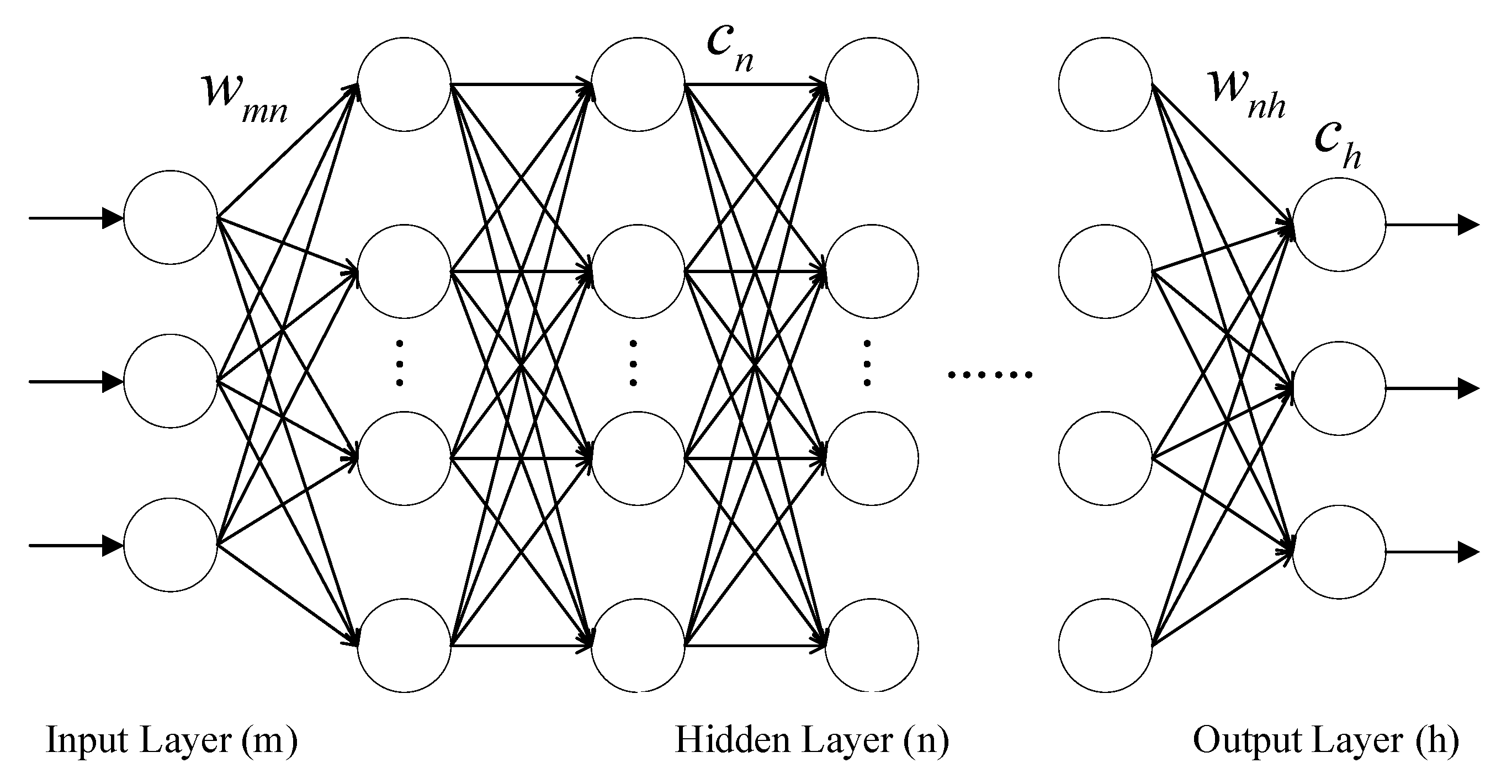
4.2. Deep Feedforward Neural Network

Recently, the neural network is widely used in the prediction of traffic volume and proposes the development of deep learning [39,40,41]. The DFNN is a deep learning model comprised of an input layer, several hidden layers, and an output layer [42,43,44]. The quantity of hidden layers defines the depth of the architecture [45]. The topological structure of the DFNN is shown in Figure 2.

The theory of the DFNN is available in past research [44,45,46]. In this section, we introduce the activation function and objective function used in the DFNN algorithm.

Firstly, the rectified linear unit (ReLU) function was selected as the activation function of hidden layers and the output layer, considering that the ReLU function has a higher computing efficiency because it only activates a fraction of the neurons in each epoch. The ReLU function has been proven to be effective at avoiding gradient vanishing and overfitting, and serves as the preferred choice when developing a neural network to solve multiple problems except for the binary classification [46,47]. The ReLU function is shown in Equation (1).

$$f\left(x\right)=\{\begin{array}{l}0x<0\\ xx\ge 0\end{array}$$

(1)

Then, the objective function was built by minimizing the loss function of mean square error, as in Equation (2).

$$\min \frac{1}{N}{\displaystyle \sum _{i=1}^N{(y_i-{\widehat{y}}_i)}^2}+\lambda \cdot R(\theta )$$

(2)

where $y_i$ represents the actual highway passenger volume and ${\widehat{y}}_i$ represents the predicted highway volume. $N$ is the number of predicted samples. $R(\cdot )$ is a regularized constraint, represented by the $L2$ norm of the parameter $\theta$, which is solved by the gradient descent method. $\lambda$ is the coefficient of regularized constraint $R(\cdot )$.

4.3. Evaluating Indicators

To better evaluate the deviation of predicted results and assess the predicted method’s performance, two indicators, MAE and RMSE, were calculated in this study. They are defined by Equations (3) and (4), respectively.

$$MAE=\frac{1}{N}{\displaystyle \sum _{i=1}^N\left|y_i-{\widehat{y}}_i\right|}$$

(3)

$$RMSE=\sqrt{\frac{1}{N}{\displaystyle \sum _{i=1}^N{(y_i-{\widehat{y}}_i)}^2}}$$

(4)

where $y_i$ and ${\widehat{y}}_i$ represent the actual highway passenger volume and the predicted highway passenger volume, respectively. $N$ is the number of predicted samples. Both MAE and RMSE represent the degree of deviation between the actual and predicted highway passenger volume. The smaller the value of MAPE and RMSE, the more accurate the predicted result.

5. Phase I: Extraction of Significant Factors

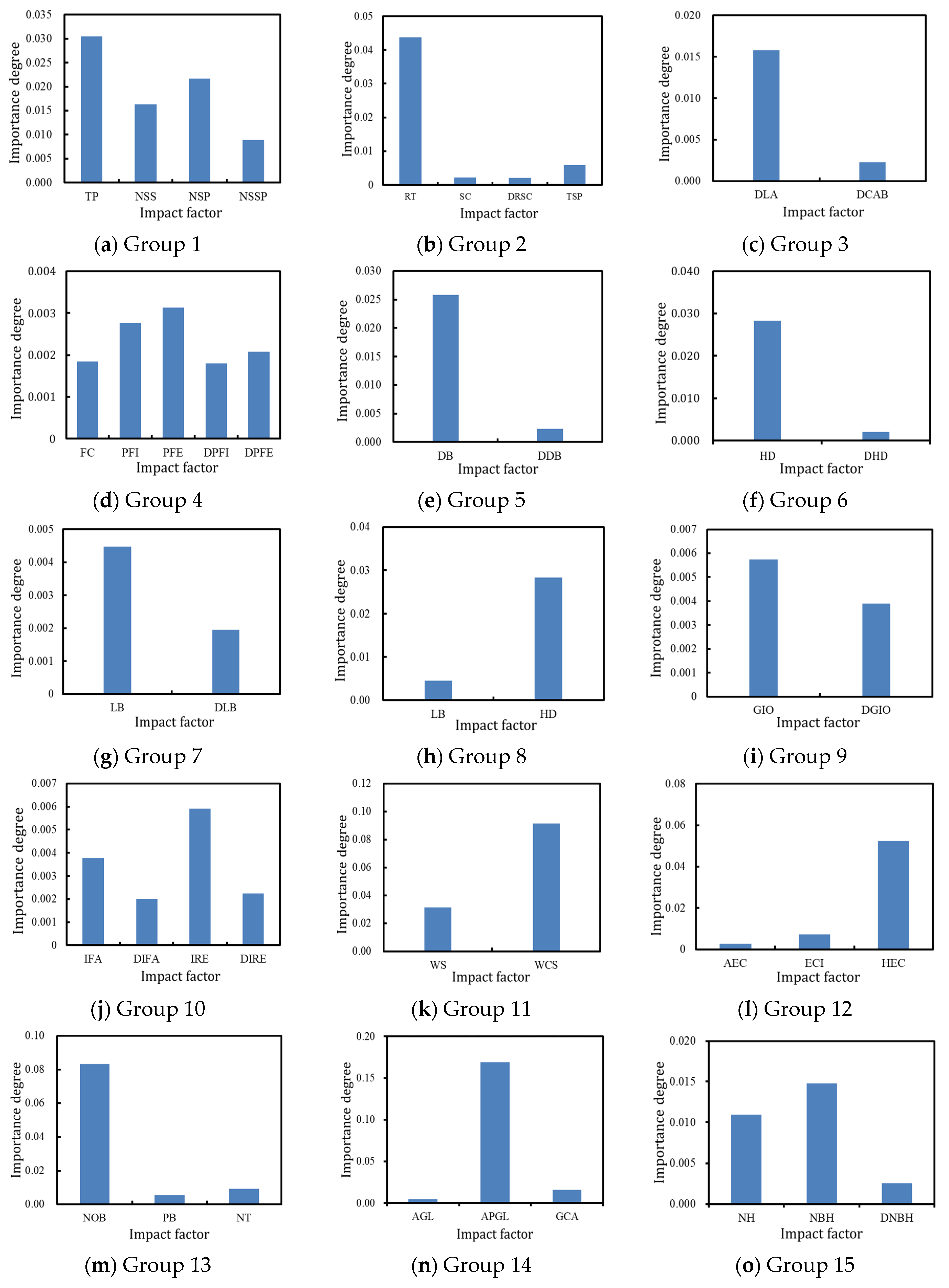
In Phase I, the RF algorithm was used for removing the highly correlated impact factors and extracting the significant impact factors. Specifically, impact factors with a high importance degree were retained and those with a low importance degree were removed. The RF algorithm has the advantage of showing the extraction of significant factors step by step and the extracted significant impact factors are interpretable, compared with some auto-encoder methods like neural networks. Finally, a dataset of significant impact factors was built for predicting highway passenger volume.

Firstly, the correlation coefficients between impact factors were calculated by correlation analysis, and fifteen groups of highly correlated impact factors were found based on the calculated correlation coefficients, which are shown in Table 1.

Table 1. Groups of highly correlated impact factors.

Group	Highly Correlated Impact Factors	Group	Highly Correlated Impact Factors
1	NSS, NSP, NSSP, TP	8	DLB, HD
2	RT, SC, DRSC, TSP	9	GIO, DGIO
		10	IFA, DIFA, IRE, DIRE
3	DLA, DCAB	11	WS, WCS
4	FC, PFI, PFE, DPFI, DPFE	12	AEC, ECI, HEC
5	DB, DDB	13	NOB, PB, NT
6	HD, DHD	14	AGL, APGL, GCA
7	LB, DLB	15	NH, NBH, DNBH

Table 1. Groups of highly correlated impact factors.

Group	Highly Correlated Impact Factors	Group	Highly Correlated Impact Factors
1	NSS, NSP, NSSP, TP	8	DLB, HD
2	RT, SC, DRSC, TSP	9	GIO, DGIO
		10	IFA, DIFA, IRE, DIRE
3	DLA, DCAB	11	WS, WCS
4	FC, PFI, PFE, DPFI, DPFE	12	AEC, ECI, HEC
5	DB, DDB	13	NOB, PB, NT
6	HD, DHD	14	AGL, APGL, GCA
7	LB, DLB	15	NH, NBH, DNBH

Then, the importance degree of highly correlated impact factors in each group was calculated with the RF algorithm, as shown in Figure 3. The horizontal axis represents impact factors in each group, and the vertical axis represents the corresponding importance degree. Only the impact factor with the largest importance degree in each group was retained, and other impact factors were removed. Consequently, 28 impact factors, including NSS, NSSP, NSP, SC, DRSC, TSP, DCAB, DPFI, DPFE, PFI, FC, DDB, DHD, DLB, LB, DGIO, IFA, DIFA, DIRE, WS, ECI, AEC, PB, NT, GCA, AGL, DNBH, and NH, were removed and the other 41 impact factors were retained. Then, the importance degree of the remaining impact factors was calculated again and sorted in order, as shown in Figure 4.

In this study, the removed proportion was set at 10%. Therefore, impact factors with importance degree rankings in the bottom 10% were removed. According to Figure 4a, the removed impact factors included RP, CPR, VISR, and DNH, and the remaining 37 impact factors were retained for the subsequent data processing.

Similarly, the importance degree of impact factors was calculated repeatedly and sorted in order, and impact factors whose importance degree ranked in the bottom 10% were removed until the importance degree of the remaining impact factors reached 0.01. The above process was repeated twice. PCGRP, IRE, LA, and PFE, and DPD, PTPT, and CLPGR were removed during these two processes, respectively, as seen in Figure 4b,c. Finally, a total of 30 impact factors were retained, and are shown in

Table 2. The extraction result of significant impact factors.

Category	Included Impact Factors
Urban economic level	GDP, RSC, RT, GIO
Urban population size and structure	TP, NSC, WPI, WSI, WTI, PD, PLPG
Per-capita income and consumption	AWW, DB, HD, WCS, HEC
Urban industrial structure	PI, SI, TI
Resource and environment	DLA, LC, NOB, APR, APGL, GCAP, NBH, NTM, CPL, VDWW, VSDE

. The category of resource and environment had more retained factors than any other, indicating that this category has a significant impact on highway passenger volume. Moreover, the importance degrees of HD, GDP, WCS, NOB, RT, HEC, TP, and TI rank in the top 25%, meaning that these eight factors significantly impact highway passenger volume.

6. Phase II: Model Prediction and Evaluation

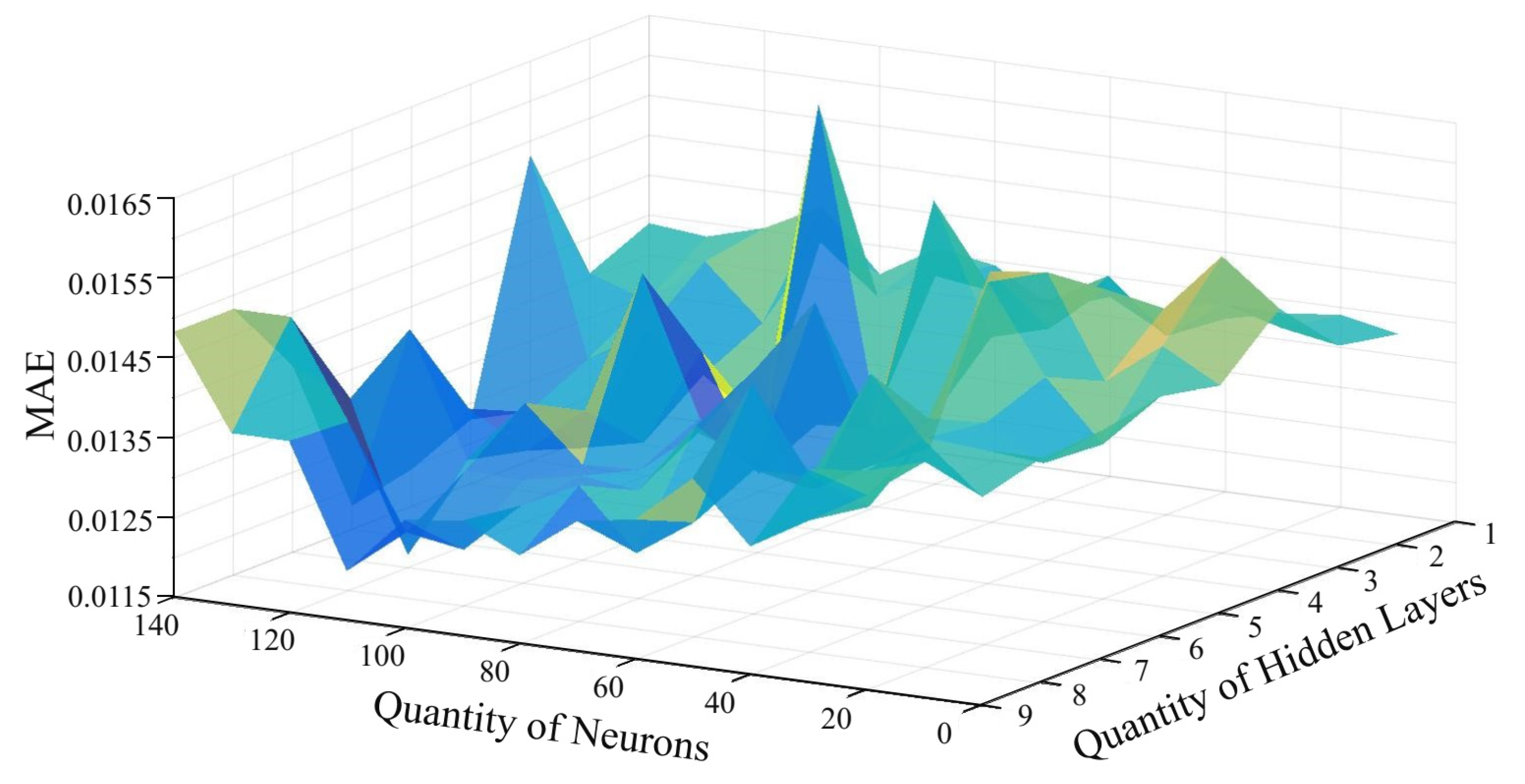
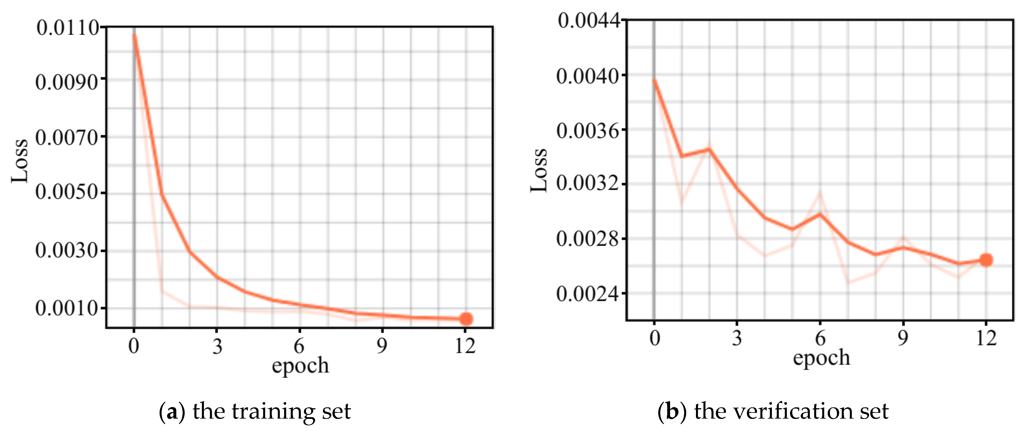
6.1. Model Prediction

With the significant impact factors selected by Phase I as input variables, Phase II developed the DFNN to predict highway passenger volume. The primary concern of developing DFNN is to determine the appropriate quantity of hidden layers and neurons in each hidden layer. In this study, the grid search method was adopted, whose initial range for the number of hidden layers was set from 1 to 10 and that for the number of neurons was set from 1 to 140. Taking MAE as an evaluating index, the result of the grid search method is shown in Figure 5.

The quantity of hidden layers and neurons with the minimum MAE is selected. Finally, the quantity of hidden layers is set to 9, and the quantity of neurons in each hidden layer is set to 120 in the DFNN of this study. Moreover, the quantity of neurons in the input layer and the output layer is set to 30 and 1, respectively, because there are 30 independent variables and 1 dependent variable.

Additionally, multiple epochs are needed for improving the predicted accuracy of the DFNN. Consequently, we continuously increased the epoch and calculated the loss of training set and verification set. When the loss of four consecutive epochs is less than 0.0001, it is considered that the training process has reached convergence and can be stopped. The loss of the training process is shown in Figure 6. Finally, the epoch of the DFNN in this study was set to 12.

Afterward, the significant impact factors were input in the developed DFNN, and the highway passenger volume was predicted. Then, evaluating indicators were calculated, showing that the MAE and RMSE of predicted highway volume from the DFNN are 2066.31 persons per day and 4176.37 persons per day, respectively.

6.2. Model Evaluation

To further evaluate the performance of the DFNN, the traditional SVM and multiple regression were used for comparison. For the SVM, the RBF kernel function whose penalty coefficient is set as 1000, and the Gamma coefficient is set as 0.001, was selected by adopting the grid search method based on the alternative sets of the kernel function, penalty coefficient, and gamma coefficient, as shown in

Table 3. The alternative sets of parameters in the SVM.

Kernel Function	Set of Penalty Coefficients
RBF	[0.001, 0.01, 0.1, 1, 10, 100, 1000]
Linear Function	[0.001, 0.01, 0.1, 1, 10, 100, 1000]
Kernel Function	Set of Gamma Coefficients
RBF	[0.0001, 0.001, 0.1, 1, 10, 100, 1000]
Linear Function	--

.

The final predicted result is shown in

Table 4. Model comparison between MAE and RMSE.

Model	MAE	RMSE
Multiple regression	2258.05	4270.29
SVM algorithm	2128.03	4225.06
DFNN	2066.31	4176.37

, both MAE and RMSE of the DFNN are less than those of the SVM and multiple regression. The DNFF reduces the MAE and RMSE by 8.49% and 2.20%, respectively, compared with the multiple regression. The DFNN reduces MAE and RMSE by 2.90% and 1.15%, respectively, compared with the SVM. The result indicates that the DFNN is more accurate in predicting highway volume than the SVM and multiple regression.

7. Conclusions

This study overcomes the limitations of existing research on predicting highway passenger volume. The main work and results of this study are as follows:

(1)

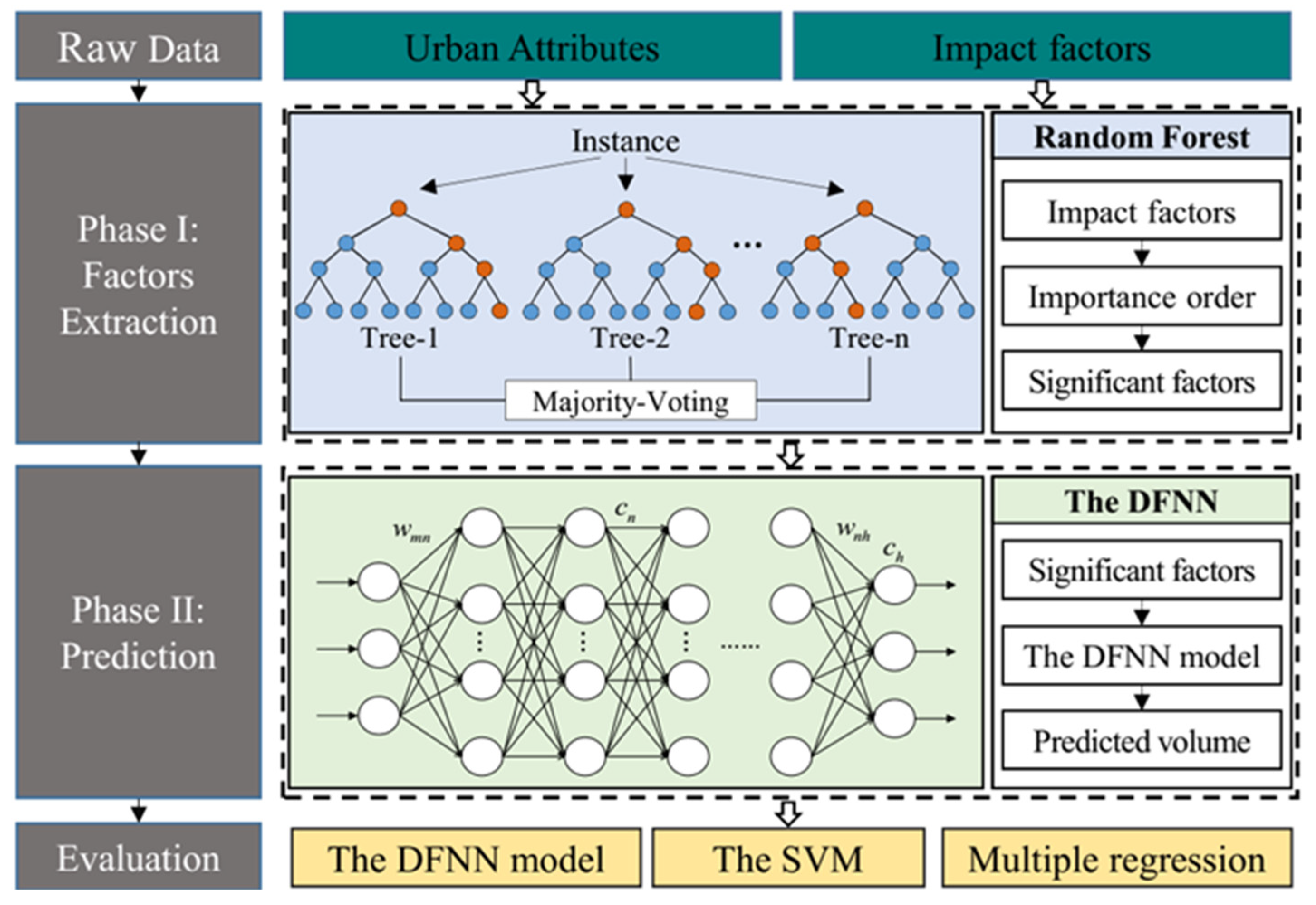
A two-phase approach, in which Phase I extracts the significant impact factors and Phase II develops a deep learning model to achieve the prediction, was proposed to predict the highway passenger volume with the dataset of multiple urban attributes;

(2)

Phase I extracted a dataset with 30 significant factors reflecting urban economic level, urban population size and structure, per-capita income and consumption, urban industrial structure, and resource and environments with the RF algorithm and proved that they have a significant impact on highway passenger volume.

(3)

Phase II developed the deep learning method, DFNN, to predict the highway passenger volume with a mean absolute error of 2066.31 persons per day, improving the predicted accuracy by 8.49% compared to the multiple regression and 2.20% compared to the SVM algorithm.

This study contributes to proposing a novel approach for predicting highway passenger volume, but limitations still exist and are worth further study. Recently, deep learning algorithms have been proposed and are expected to be utilized for further improving the predicted accuracy of highway passenger volume as well as increasing the interpretability. As the statistical yearbook only publishes the annual statistics, it is difficult to make a detailed analysis of highway passenger volume in quarters or months. Moreover, it is possible to find data mutation caused by the change of statistical caliber in the statistical yearbook, which affects the predicted accuracy. Therefore, other new datasets can be considered to introduce into future research for more accurate analysis.

References

1. Lin, L.; Hao, Z.; Post, C.J.; Mikhailova, E.A.; Yu, K.; Yang, L.; Liu, J. Monitoring Land Cover Change on a Rapidly Urbanizing Island Using Google Earth Engine. Appl. Sci. 2020, 10, 7336. [Google Scholar] [CrossRef]
2. Bong, A.; Premaratne, G. Regional Integration and Economic Growth in Southeast Asia. Glob. Bus. Rev. 2018, 19, 1403–1415. [Google Scholar] [CrossRef]
3. Liu, J.; Wu, N.; Qiao, Y.; Li, Z. A scientometric review of research on traffic forecasting in transportation. IET Intell. Transp. Syst. 2021, 15, 1–16. [Google Scholar] [CrossRef]
4. Chen, J.; Li, D.; Zhang, G.; Zhang, X. Localized Space-Time Autoregressive Parameters Estimation for Traffic Flow Prediction in Urban Road Networks. Appl. Sci. 2018, 8, 277. [Google Scholar] [CrossRef] [Green Version]
5. Xiang, Y.; Xu, C.; Yu, W.; Wang, S.; Hua, X.; Wang, W. Investigating Dominant Trip Distance for Intercity Passenger Transport Mode Using Large-Scale Location-Based Service Data. Sustainability 2019, 11, 5325. [Google Scholar] [CrossRef] [Green Version]
6. Li, X.; Tang, J.; Hu, X.; Wang, W. Assessing intercity multimodal choice behavior in a Touristy City: A factor analysis. J. Transp. Geogr. 2020, 86, 102776. [Google Scholar] [CrossRef]
7. Soltani, A.; Allan, A. Analyzing the Impacts of Microscale Urban Attributes on Travel: Evidence from Suburban Adelaide, Australia. J. Urban Plan. Dev. 2006, 132, 132–137. [Google Scholar] [CrossRef]
8. Miao, D.; Wang, W.; Xiang, Y.; Hua, X.; Yu, W. Analysis on the Influencing Factors of Traffic Mode Choice Behavior for Regional Travel in China. In CICTP 2020; American Society of Civil Engineers (ASCE): Virginia, VA, USA, 2020; pp. 3969–3980. [Google Scholar]
9. Nikravesh, A.Y.; Ajila, S.A.; Lung, C.-H.; Ding, W. Mobile Network Traffic Prediction Using MLP, MLPWD, and SVM. In Proceedings of the 2016 IEEE International Congress on Big Data (BigData Congress), Washington, DC, USA, 5–8 December 2016; Institute of Electrical and Electronics Engineers (IEEE): San Francisco, CA, USA, 2016; pp. 402–409. [Google Scholar]
10. Gu, Y.; Lu, W.; Xu, X.; Qin, L.; Shao, Z.; Zhang, H. An improved Bayesian combination model for short-term traffic prediction with deep learning. IEEE Trans. Intell. Transp. Syst. 2019, 21, 1332–1342. [Google Scholar] [CrossRef]
11. Lin, L.; Handley, J.; Gu, Y.; Zhu, L.; Wen, X.; Sadek, A.W. Quantifying uncertainty in short-term traffic prediction and its application to optimal staffing plan development. Transp. Res. Part C Emerg. Technol. 2018, 92, 323–348. [Google Scholar] [CrossRef]
12. Brueckner, J.K. Airline Traffic and Urban Economic Development. Urban Stud. 2003, 40, 1455–1469. [Google Scholar] [CrossRef]
13. Caceres, N.; Romero, L.M.; Morales, F.J.; Reyes, A.; Benitez, F.G. Estimating traffic volumes on intercity road locations using roadway attributes, socioeconomic features and other work-related activity characteristics. Transportation 2018, 45, 1449–1473. [Google Scholar] [CrossRef]
14. Chen, W.; Liu, W.; Ke, W.; Wang, N. Understanding spatial structures and organizational patterns of city networks in China: A highway passenger flow perspective. J. Geogr. Sci. 2018, 28, 477–494. [Google Scholar] [CrossRef] [Green Version]
15. Antipova, A.; Wang, F.; Wilmot, C. Urban land uses, socio-demographic attributes and commuting: A multilevel modeling approach. Appl. Geogr. 2011, 31, 1010–1018. [Google Scholar] [CrossRef]
16. Low, J.M.; Lee, B.K. A Data-Driven Analysis on the Impact of High-Speed Rails on Land Prices in Taiwan. Appl. Sci. 2020, 10, 3357. [Google Scholar] [CrossRef]
17. Limtanakool, N.; Dijst, M.; Schwanen, T. The influence of socioeconomic characteristics, land use and travel time considera-tions on mode choice for medium- and longer-distance trips. J. Transp. Geogr. 2006, 14, 327–341. [Google Scholar] [CrossRef]
18. De Witte, A.; Hollevoet, J.; Dobruszkes, F.; Hubert, M.; Macharis, C. Linking modal choice to motility: A comprehensive review. Transp. Res. Part A Policy Pract. 2013, 49, 329–341. [Google Scholar] [CrossRef]
19. Tian, Y.; Yao, X. Urban form, traffic volume, and air quality: A spatiotemporal stratified approach. Environ. Plan. B Urban Anal. City Sci. 2021, 2399808321995822. [Google Scholar] [CrossRef]
20. Li, Z.; Wang, Y.; Zhao, S. Study of Intercity Travel Characteristics in Chinese Urban Agglomeration. Int. Rev. Spat. Plan. Sustain. Dev. 2015, 3, 75–85. [Google Scholar] [CrossRef] [Green Version]
21. Lee, D.; Derrible, S.; Pereira, F.C. Comparison of Four Types of Artificial Neural Network and a Multinomial Logit Model for Travel Mode Choice Modeling. Transp. Res. Rec. J. Transp. Res. Board 2018, 2672, 101–112. [Google Scholar] [CrossRef] [Green Version]
22. Bhatta, B.P.; Larsen, O.I. Errors in variables in multinomial choice modeling: A simulation study applied to a multinomial logit model of travel mode choice. Transp. Policy 2011, 18, 326–335. [Google Scholar] [CrossRef] [Green Version]
23. Huang, B.; Fioreze, T.; Thomas, T.; Van Berkum, E. Multinomial logit analysis of the effects of five different app-based incentives to encourage cycling to work. IET Intell. Transp. Syst. 2018, 12, 1421–1432. [Google Scholar] [CrossRef]
24. Jourquin, B. Mode choice in strategic freight transportation models: A constrained Box–Cox meta-heuristic for multivariate utility functions. Transp. A Transp. Sci. 2021, 1–21. [Google Scholar] [CrossRef]
25. Elmorssy, M.; Onur, T.H. Modelling Departure Time, Destination and Travel Mode Choices by Using Generalized Nested Logit Model: Discretionary Trips. Int. J. Eng. 2020, 33, 186–197. [Google Scholar] [CrossRef]
26. Rahmat, O.K. Modeling of intercity transport mode choice behavior in Libya: A binary logit model for business trips by private car and intercity bus. Aust. J. Basic Appl. Sci. 2013, 7, 302–311. [Google Scholar]
27. Wang, R.; Zhang, T.; Liu, S.; Zhang, Z. Prediction of Passenger Traffic Volume Sharing Rate Based on Logit Model. In Proceedings of the 3rd International Conference on Information Technology and Intelligent Transportation Systems (ITITS 2018), Xi’an, China, 15–16 September 2018; p. 296. [Google Scholar]
28. Harker, P.T.; Friesz, T.L. Prediction of intercity freight flows, I: Theory. Transp. Res. Part B Methodol. 1986, 20, 139–153. [Google Scholar] [CrossRef]
29. Li, H.-L.; Lin, M.-K.; Wang, Q.-C. Passenger Flow Prediction Model of Intercity Railway Based on G-BP Network. In Lecture Notes in Electrical Engineering; Springer Science and Business Media LLC: Berlin/Heidelberg, Germany, 2020; pp. 859–870. [Google Scholar]
30. Xie, B.; Sun, Y.; Huang, X.; Yu, L.; Xu, G. Travel Characteristics Analysis and Passenger Flow Prediction of Intercity Shuttles in the Pearl River Delta on Holidays. Sustainability 2020, 12, 7249. [Google Scholar] [CrossRef]
31. Lv, Y.; Duan, Y.; Kang, W.; Li, Z.; Wang, F.-Y. Traffic Flow Prediction With Big Data: A Deep Learning Approach. IEEE Trans. Intell. Transp. Syst. 2014, 16, 1–9. [Google Scholar] [CrossRef]
32. Moreira-Matias, L.; Gama, J.; Ferreira, M.; Mendes-Moreira, J.; Damas, L. Predicting Taxi–Passenger Demand Using Streaming Data. IEEE Trans. Intell. Transp. Syst. 2013, 14, 1393–1402. [Google Scholar] [CrossRef] [Green Version]
33. Yin, X.; Wu, G.; Wei, J.; Shen, Y.; Qi, H.; Yin, B. Deep Learning on Traffic Prediction: Methods, Analysis and Future Directions; IEEE: New York City, NY, USA, 2021. [Google Scholar]
34. Tortum, A.; Yayla, N.; Gökdağ, M. The modeling of mode choices of intercity freight transportation with the artificial neural networks and adaptive neuro-fuzzy inference system. Expert Syst. Appl. 2009, 36, 6199–6217. [Google Scholar] [CrossRef]
35. Allard, R.F.; Moura, F. The Incorporation of Passenger Connectivity and Intermodal Considerations in Intercity Transport Planning. Transp. Rev. 2016, 36, 251–277. [Google Scholar] [CrossRef]
36. Le, H.T.; West, A.; Quinn, F.; Hankey, S. Advancing cycling among women: An exploratory study of North American cyclists. J. Transp. Land Use 2019, 12, 355–374. [Google Scholar] [CrossRef] [Green Version]
37. Pal, M. Random forest classifier for remote sensing classification. Int. J. Remote. Sens. 2005, 26, 217–222. [Google Scholar] [CrossRef]
38. Sun, J.; Sun, J. Real-time crash prediction on urban expressways: Identification of key variables and a hybrid support vector machine model. IET Intell. Transp. Syst. 2016, 10, 331–337. [Google Scholar] [CrossRef]
39. Xu, C.; Ji, J.; Liu, P. The station-free sharing bike demand forecasting with a deep learning approach and large-scale datasets. Transp. Res. Part C Emerg. Technol. 2018, 95, 47–60. [Google Scholar] [CrossRef]
40. Xie, Z.; Zhu, J.; Wang, F.; Li, W.; Wang, T. Long short-term memory based anomaly detection: A case study of China railway passen-ger ticketing system. IET Intell. Transp. Syst. 2020. [Google Scholar] [CrossRef]
41. Liu, P.; Zhang, Y.; Kong, D.; Yin, B. Improved Spatio-Temporal Residual Networks for Bus Traffic Flow Prediction. Appl. Sci. 2019, 9, 615. [Google Scholar] [CrossRef] [Green Version]
42. Oliveira, T.P.; Barbar, J.S.; Soares, A.S. Computer network traffic prediction: A comparison between traditional and deep learning neural networks. Int. J. Big Data Intell. 2016, 3, 28. [Google Scholar] [CrossRef]
43. Glorot, X.; Bengio, Y. Understanding the difficulty of training deep feedforward neural networks. In Proceedings of the Thirteenth International Conference on Artificial Intelligence and Statistics, Chia Laguna Resort, Sardinia, Italy, 13–15 May 2010; pp. 249–256. [Google Scholar]
44. Gupta, T.K.; Raza, K. Optimizing Deep Feedforward Neural Network Architecture: A Tabu Search Based Approach. Neural Process. Lett. 2020, 51, 2855–2870. [Google Scholar] [CrossRef]
45. Loiseau, P.; Boultifat, C.N.E.; Chevrel, P.; Claveau, F.; Espié, S.; Mars, F. Rider model identification: Neural networks and quasi-LPV models. IET Intell. Transp. Syst. 2020, 14, 1259–1264. [Google Scholar] [CrossRef]
46. Agarap, A.F. Deep learning using rectified linear units (relu). arXiv 2018, arXiv:1803.08375. [Google Scholar]
47. Eckle, K.; Schmidt-Hieber, J. A comparison of deep networks with ReLU activation function and linear spline-type methods. Neural Netw. 2019, 110, 232–242. [Google Scholar] [CrossRef] [PubMed]
Figure 1. The flow diagram of the designed framework.
Applsci 11 06248 g001
Figure 2. The topological structure of the DFNN algorithm.
Applsci 11 06248 g002
Figure 3. The importance degrees of significantly correlated variables in each group.
Applsci 11 06248 g003
Figure 4. Importance degrees of impact factors. (a) The first iteration. (b) The second iteration. (c) The third iteration.
Applsci 11 06248 g004
Figure 5. The result of grid search method for determining hidden layers and neurons.
Applsci 11 06248 g005
Figure 6. The result of loss for determining epoch.
Applsci 11 06248 g006