Continuous Control Set Predictive Current Control for Induction Machine

Abstract

A speed tracking control method for induction machine is shown in this paper. The method consists of outer speed control loop and inner current control loop. Model predictive current control method without the need for calculation of the weighing factors is utilized for the inner control loop, which generates a continuous set of voltage reference values that can be modulated and applied by the inverter to the induction machine. Interesting parallels are drawn between the developed method and state feedback principles that helped with the analysis of the stability and controllability. Simple speed and rotor flux estimator is implemented that helps achieve sensorless control. Simulation is conducted and the method shows great performance for speed tracking in a steady state, and during transients as well. Additionally, compared to the finite control set predictive current control, it shows less harmonic content in the generated torque on the rotor shaft.

1. Introduction

Induction machines are crucial part of today’s world industry because of their robustness and power per volume. Thanks to the research in the control field, they achieve satisfying reference tracking and can easily replace DC machines. Methods that revolutionized the field of induction machine control are field oriented control (FOC), developed in the seventies by Hasse and Blaschke which are presented in their Ph.D. thesis [1,2] and direct torque control (DTC), developed in the eighties by Takahashi and Noguchi [3]. From there, field of research for induction machine control expanded and many more authors contributed to the progress and countless variations of the methods emerged. At the time, model predictive control (MPC) was used in slow chemical processes, due to high computational burden that computers could not handle, but, with the development of digital signal processors, these methods could slowly be implemented to control fast processes. Authors Vazquez et al. made a nice overview of the subject in their review paper [4], where they classified different finite and continuous control set methods. Extended classification of the MPC can be found in [5]. Application of finite control set MPC in different types of power converters is shown in papers [6] by Kouro et al. and [7] by Rodriguez et al. From these papers, one important note can be concluded, which is that plants can be controlled using MPC by finite or continuous command control sets. Since the fields of power electronics and drives use discrete switching of the converters to control the plants, any of those two methods can be utilized. In the field of MPC for induction machines, two distinct methods can be recognized: predictive torque control (PTC) and predictive current control (PCC). There is abundance of important comparison papers that investigate these methods and compare them to classical methods. Authors Wang et al. made a comparison of FOC, DTC, PCC, and PTC in [8], while authors Kennel et al. contributed with comprehensive comparisons of FOC, DTC, and PTC in [9]. Authors Rodriguez et al. compared FOC and PTC in [10], while Wang et al. made a comparison of PTC with PCC and DTC in papers [11,12]. A lot of papers emerged with the attempts to improve upon the existing induction machine MPC methods. Authors Englert et al. developed a method for optimal setpoint calculation for the PTC in [13]. It is known that in PTC, a weighing factor must exist in the cost function in order to penalize torque and flux errors. Authors of [14,15] improve the methods to eliminate the weighing factor calculation. Authors of [16,17,18], took interesting approaches to further optimize the method where the switch-on on time of the optimal voltage vector is calculated, so that the torque ripple is minimized. There is much more content on PTC that a reader is referred to in papers such as [19], where authors use combination of Kalman filter and standard PTC for current and flux estimation, and [20], where authors improve the performance of the PTC by deriving an algorithm for state estimation at longer predictive horizon. Regarding PCC, a lot of papers are published where authors improve upon existing methods. Authors Wang et al. use universal proportional integral observer instead of PI speed regulator in [21] to improve the load torque disturbance rejection and in [22] they modify it to deal with parameter uncertainties. Authors of [23] improve the PCC for low sampling time controllers by adjusting the discrete predicting plant model. Authors Wang et al. improved upon the method by replacing the conventional speed PI controller with extended high-gain state observer in [24] and Luenberger observer in [25] to enable encoderless operation. All of these methods are based on the finite control set MPC, that commands variable switching frequency to the converter, which increases the risk of resonance and torque ripple on the machine. There are a few papers that deal with continuous control set MPC. One of such papers is [26], published by Vafaie et al. where a classification of the continuous control set methods is conducted. In [27,28], an LQR approach to PCC is applied where weighing matrices in the cost functions exist. Authors Ahmed et al. describe a simple approach to continuous control set PCC in [29,30], where a specific weighing factor matrix is calculated in order to limit commanded stator voltage of the induction machine. These methods eliminate the problems that are introduced by finite control set methods.

In this paper, authors present a continuous control set predictive current control of the induction machine without the need for calculation of the weighing factors. Stability of the method is analyzed and further possibilities that could be implemented are highlighted. In Section 2, the induction machine model is presented. In Section 3, control structure is developed and the estimator design is shown. In Section 4 stability and controllability analysis are conducted and in Section 5, simulation results are shown and commented. In Section 6, authors discuss the results, highlight the possibilities of the method and develop a basis for the future work.

2. Induction Machine Model

Dynamic mathematical model of the induction machine is described by Equations (1)–(4). The reader is referred to [31] for further understanding of the model.

$$\begin{array}{c}{\mathit{v}}_{s\alpha \beta }={\mathit{R}}_s{\mathit{i}}_{s\alpha \beta }+\frac{\mathrm{d}}{\mathrm{d}t}{\mathit{\psi }}_{s\alpha \beta }\end{array}$$

(1)

$$\begin{array}{c}0={\mathit{R}}_r{\mathit{i}}_{r\alpha \beta }+\mathit{j}p{\omega }_r{\mathit{\psi }}_{r\alpha \beta }+\frac{\mathrm{d}}{\mathrm{d}t}{\mathit{\psi }}_{r\alpha \beta }\end{array}$$

(2)

$$\begin{array}{c}J\frac{\mathrm{d}}{\mathrm{d}t}{\omega }_r=T_e-T_l\end{array}$$

(3)

$$\begin{array}{c}{T}_e=\frac{3}{2}p({\psi }_{s\alpha }{i}_{s\beta }-{\psi }_{s\beta }{i}_{s\alpha })\end{array}$$

(4)

The model is written in stationary $\alpha \beta$-reference frame where ${\mathit{v}}_{s\alpha \beta }={[v_{s\alpha }\hspace{1em}{v}_{s\beta }]}^T$ describes stator voltage vector, ${\mathit{i}}_{s\alpha \beta }={[i_{s\alpha }\hspace{1em}{i}_{s\beta }]}^T$ and ${\mathit{i}}_{r\alpha \beta }={[i_{r\alpha }\hspace{1em}{i}_{r\beta }]}^T$ describe stator and rotor current vector, ${\mathit{\psi }}_{s\alpha \beta }={[{\psi }_{s\alpha }\hspace{1em}{\psi }_{s\beta }]}^T$ and ${\mathit{\psi }}_{r\alpha \beta }={[{\psi }_{r\alpha }\hspace{1em}{\psi }_{r\beta }]}^T$ describe stator and rotor flux linkages. J is inertia constant of the machine, ${\omega }_r$ is rotor shaft speed, p is number of pole pairs, $T_e$ is electromechanical torque and $T_l$ is load torque. ${\mathit{R}}_s$ and ${\mathit{R}}_r$ are stator and rotor resistance matrices, while $\mathit{j}$ represents the rotation matrix described by Equation (5).

$${\mathit{R}}_s=\left[\begin{array}{c}{R}_s\hspace{1em}0\\ 0\hspace{1em}{R}_s\end{array}\right]{\mathit{R}}_r=\left[\begin{array}{c}{R}_r\hspace{1em}0\\ 0\hspace{1em}{R}_r\end{array}\right]\mathit{j}=\left[\begin{array}{c}0\hspace{1em}-1\\ 1\hspace{1em}0\end{array}\right]$$

(5)

The flux linkages are depicted by Equations (6) and (7).

$$\begin{array}{c}{\mathit{\psi }}_{s\alpha \beta }=L_s{\mathit{i}}_{s\alpha \beta }+L_m{\mathit{i}}_{r\alpha \beta }\end{array}$$

(6)

$$\begin{array}{c}{\mathit{\psi }}_{r\alpha \beta }=L_r{\mathit{i}}_{r\alpha \beta }+L_m{\mathit{i}}_{s\alpha \beta }\end{array}$$

(7)

where $L_s$, $L_r$ and $L_m$ represent stator, rotor, and mutual inductance, respectively.

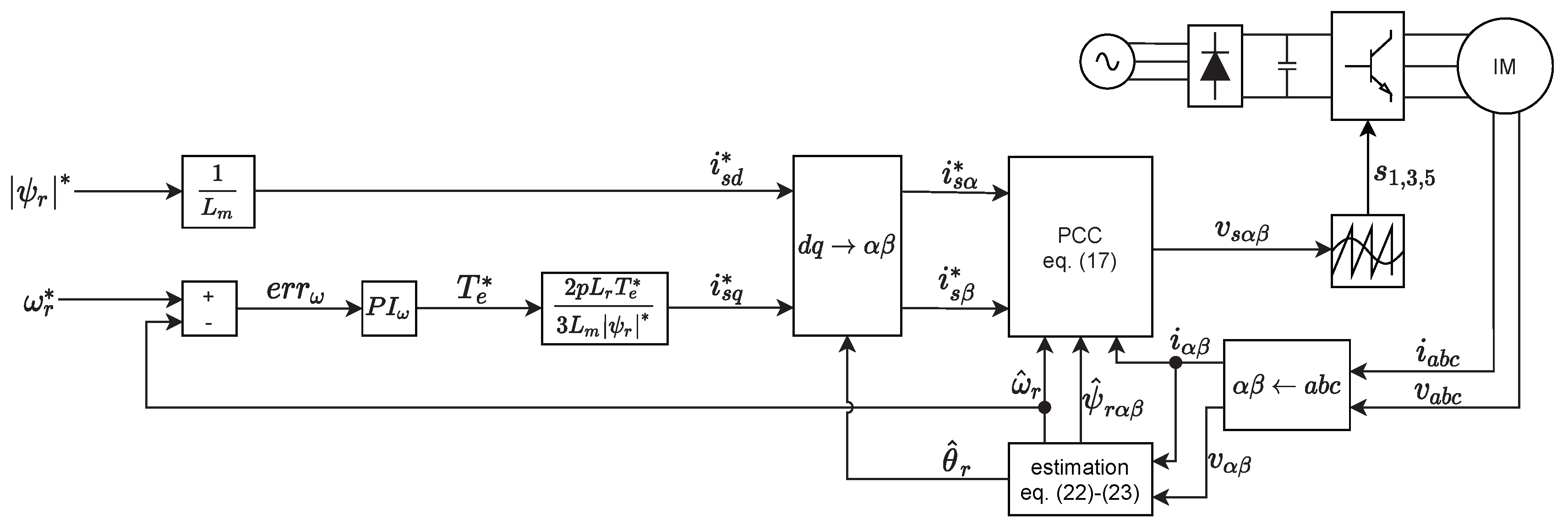
3. Control Structure

When modeling induction machines several state variables can be chosen to represent the state. For the proposed control structure, stator current, and rotor flux $\alpha \beta$-components are chosen. Additionally, the control structure is developed as cascade regulation with inner and outer control loops. Outer control loop is classic speed regulation via PI regulator that generates torque reference, while inner loop is the predictive current control via the proposed method. Any kind of model predictive control should be comprised of cost function that is minimized by selecting the optimal input to the system. Classic cost function that is used for predictive current control for induction machines driven by two-level voltage inverters can be found in papers, such as [32] or [11], and is shown by Equation (8):

$$g\left(v_i\right)=\sum _{j=0}^h\left(\right|i_{\alpha }^{*}-i_{\alpha }[k+j]|+|i_{\beta }^{*}-i_{\beta }[k+j]\left|\right),i\in \{0,1,...,7\}$$

(8)

where variables with the star superscript represent reference values, $i_{\alpha }[k+h]$ and $i_{\beta }[k+h]$ represent stator current components calculated at k-th sample for h future samples and $v_i$ is one of eight possible voltage vectors applied to the machine during one switching period that minimizes the cost function. This kind of PCC is also called finite control set PCC and it has the before-mentioned drawbacks. In order to derive continuous control set PCC, a continuous control signal should be generated by the regulator that can be modulated by the inverter. Induction machine model derived for this purpose is explained in the following subsection.

3.1. Deriving the Control Algorithm for the Inner Control Loop

By expressing the rotor current from (7) and plugging it into (2), Equation (9) that describes rotor flux dynamics is derived:

$$\frac{\mathrm{d}}{\mathrm{d}t}{\mathit{\psi }}_{r\alpha \beta }=\frac{L_m}{{\tau }_r}{\mathit{i}}_{s\alpha \beta }-(\frac{1}{{\tau }_r}\mathit{I}-\mathit{j}p{\omega }_r){\mathit{\psi }}_{r\alpha \beta }$$

(9)

where ${\tau }_r=\frac{L_r}{R_r}$ represents the rotor time constant and $\mathit{I}$ is identity matrix. Furthermore, by plugging (6) and (7) into (1) and replacing the rotor flux derivative with the expression (9), following equation for stator current dynamics is derived:

$$\frac{\mathrm{d}}{\mathrm{d}t}{\mathit{i}}_{s\alpha \beta }=-\frac{R_s+\frac{L_m^2}{L_r{\tau }_r}}{\sigma L_s}{\mathit{i}}_{s_{\alpha }\beta }+\frac{L_m\sigma L_s}{L_r}(\frac{1}{{\tau }_r}\mathit{I}-\mathit{j}p{\omega }_r){\mathit{\psi }}_{r\alpha \beta }+\frac{1}{\sigma L_s}{\mathit{v}}_{s_{\alpha }\beta }$$

(10)

where $\sigma =1-\frac{L_m^2}{L_s{L}_r}$ represents leakage inductance factor. By arranging Equations (9) and (10) into a state-space form, following equation is derived:

$$\frac{\mathrm{d}}{\mathrm{d}t}\mathit{x}=\mathit{A}\left({\omega }_r\right)\mathit{x}+\mathit{B}\mathit{u}$$

(11)

where $\mathit{x}$ is a state vector, $\mathit{A}$ is state matrix, $\mathit{B}$ is input matrix and $\mathit{u}$ is input vector, defined by (12).

$$\begin{array}{cc}\hfill \mathit{x}=\left[\begin{array}{c}{i}_{s\alpha }\\ i_{s\beta }\\ {\psi }_{r\alpha }\\ {\psi }_{r\beta }\end{array}\right]\hfill & \mathit{u}=\left[\begin{array}{c}{v}_{s\alpha }\\ v_{s\beta }\end{array}\right]\\ \mathit{A}\left({\omega }_r\right)=\left[\begin{array}{cccc}-\frac{R_s+\frac{L_m^2}{L_r{\tau }_r}}{\sigma L_s}& 0& \frac{L_m\sigma L_s}{L_r{\tau }_r}& \frac{L_m\sigma L_{s}p{\omega }_r}{L_r}\\ 0& -\frac{R_s+\frac{L_m^2}{L_r{\tau }_r}}{\sigma L_s}& -\frac{L_m\sigma L_{s}p{\omega }_r}{L_r}& \frac{L_m\sigma L_s}{L_r{\tau }_r}\\ \frac{L_m}{{\tau }_r}& 0& -\frac{1}{{\tau }_r}& -p{\omega }_r\\ 0& \frac{L_m}{{\tau }_r}& p{\omega }_r& -\frac{1}{{\tau }_r}\end{array}\right]& \mathit{B}=\left[\begin{array}{cc}\frac{1}{\sigma L_s}& 0\\ 0& \frac{1}{\sigma L_s}\\ 0& 0\\ 0& 0\end{array}\right]\end{array}$$

(12)

In order to implement the predictive current control, the machine model should be discretized. Using forward euler discretization (13), it is possible to predict state values of the next sample based on the values of the current sample. Since the $\alpha -\beta$-component values of the stator current are of interest, only first two rows of the state and input matrix will be considered. After discretization with sampling time $T_s$ and state and input matrices truncation, the Equation (14) is derived and it will be used in the proposed method:

$$\begin{array}{c}\hfill \begin{array}{c}\mathit{x}[k+1]={\mathit{A}}_d\left({\omega }_r\right)\mathit{x}\left[k\right]+{\mathit{B}}_d\mathit{u}\left[k\right]\\ {\mathit{A}}_d\left({\omega }_r\right)=\mathit{I}+T_s\mathit{A}\left({\omega }_r\right){\mathit{B}}_d=T_s\mathit{B}\end{array}\end{array}$$

(13)

$$\begin{array}{ccc}\hfill \left[\begin{array}{c}\hfill i_{s\alpha }[k+1]\\ i_{s\beta }[k+1]\end{array}\right]& =\left[\begin{array}{cccc}1-\frac{(R_s+\frac{L_m^2}{L_r{\tau }_r})T_s}{\sigma L_s}& \hfill 0\hfill & \frac{L_m\sigma L_s{T}_s}{L_r{\tau }_r}& \frac{L_m\sigma L_{s}p{\omega }_r{T}_s}{L_r}\\ \hfill 0\hfill & 1-\frac{(R_s+\frac{L_m^2}{L_r{\tau }_r})T_s}{\sigma L_s}& -\frac{L_m\sigma L_{s}p{\omega }_r{T}_s}{L_r}& \frac{L_m\sigma L_s{T}_s}{L_r{\tau }_r}\end{array}\right]& \left[\begin{array}{c}{i}_{s\alpha }\left[k\right]\\ \hfill i_{s\beta }\left[k\right]\\ \hfill {\psi }_{r\alpha }\left[k\right]\\ \hfill {\psi }_{r\beta }\left[k\right]\end{array}\right]\\ \hfill & +\left[\begin{array}{cc}\frac{T_s}{\sigma L_s}& \hfill 0\\ \hfill 0& \frac{T_s}{\sigma L_s}\hfill \end{array}\right] \left[\begin{array}{c}\hfill v_{s\alpha }\left[k\right]\\ \hfill v_{s\beta }\left[k\right]\end{array}\right]\hfill & \end{array}$$

(14)

To derive model predictive control law, two cost functions are used, each representing the square error between reference and estimated current of the $\alpha \beta$-reference frame:

$$\mathit{G}=\left[\begin{array}{c}{g}_{\alpha }\\ g_{\beta }\end{array}\right]=\left[\begin{array}{c}{(i_{\alpha }^{*}\left[k\right]-i_{\alpha }[k+1])}^2\\ {(i_{\beta }^{*}\left[k\right]-i_{\beta }[k+1])}^2\end{array}\right]$$

(15)

In order to find optimal $\alpha \beta$ stator voltage components that minimize $\mathit{G}$, it is convenient to plug (14) into (15) and obtain the optimal voltage by solving (16).

$$\frac{\partial \mathit{G}}{\partial {\mathit{v}}_{\alpha \beta }}=0$$

(16)

By doing this, optimal voltage can be expressed as shown in Equation (17):

$$\begin{array}{c}\hfill \begin{array}{c}{\mathit{v}}_{\alpha \beta }^{*}[k+1]={\mathit{K}}_d\left({\omega }_r\right)\mathit{x}\left[k\right]+{\mathit{E}}_d{\mathit{i}}_{\alpha \beta }^{*}[k+1]\\ {\mathit{K}}_d\left({\omega }_r\right)=\left[\begin{array}{cccc}{R}_s+\frac{L_m^2}{L_r{\tau }_r}-\frac{\sigma L_s}{T_s}& 0& -\frac{L_m}{L_r{\tau }_r}& -\frac{L_{m}p{\omega }_r}{L_r}\\ 0& R_s+\frac{L_m^2}{L_r{\tau }_r}-\frac{\sigma L_s}{T_s}& \frac{L_{m}p{\omega }_r}{L_r}& -\frac{L_m}{L_r{\tau }_r}\end{array}\right]{\mathit{E}}_d=\left[\begin{array}{cc}\frac{\sigma L_s}{T_s}& 0\\ 0& \frac{\sigma L_s}{T_s}\end{array}\right]\end{array}\end{array}$$

(17)

where ${\mathit{v}}_{\alpha \beta }^{*}[k+1]={[v_{\alpha }^{*}[k+1]\hspace{1em}{v}_{\beta }^{*}[k+1]]}^T$ represent vector of optimal input voltage and ${\mathit{i}}_{\alpha \beta }^{*}[k+1]={[i_{\alpha }^{*}[k+1]\hspace{1em}{i}_{\beta }^{*}[k+1]]}^T$ represent the vector of reference current in $\alpha \beta$-reference frame. In the following subsection, an algorithm for calculation of stator current reference signal in $\alpha \beta$-reference frame will be shown.

3.2. Outer Control Loop Algorithm

To produce stator current reference values, methods from the classical rotor field oriented control in $dq$-reference frame can be applied. In other words, one can calculate d-component of the reference current from the rotor flux reference by using Equation (18) and q-component from the torque reference by using Equation (19). To transform these values from $dq$ into $\alpha \beta$-reference frame, Equation (20) is used, where ${\theta }_r$ represents angle between rotor flux vector and $\alpha$-axis.

$$i_{sd}^{*}=\frac{|{\psi }_r{|}^{*}}{L_m}$$

(18)

$$i_{sq}^{*}=\frac{2p{L}_r{T}_e^{*}}{3L_m{\left|{\psi }_r\right|}^{*}}$$

(19)

$$\left[\begin{array}{c}{i}_{s\alpha }\\ i_{s\beta }\end{array}\right]=\left[\begin{array}{cc}cos\left({\theta }_r\right)& -sin\left({\theta }_r\right)\\ sin\left({\theta }_r\right)& cos\left({\theta }_r\right)\end{array}\right]\hspace{1em}\left[\begin{array}{c}{i}_{sd}\\ i_{sq}\end{array}\right]$$

(20)

In this paper, optimal selection of the rotor flux is not considered so the flux reference $|{\psi }_r^{*}|$ will be set to constant value, while torque reference $T_e^{*}$ is going to be generated from rotor speed error using PI regulator as shown in Equation (21). The purpose of the regulator is to reduce the impact of the disturbance on the system, which is in this case the load torque.

$$T_e^{*}=({\omega }_r-{\widehat{\omega }}_r)(K_{P\omega }-\frac{K_{I\omega }}{s})$$

(21)

where s represents the integration in Laplace domain, $K_{P\omega }$ and $K_{I\omega }$ represent speed PI regulator gains and ${\widehat{\omega }}_r$ represents estimated rotor speed value.

3.3. Rotor Flux and Speed Estimation

Estimator is essential part for any type of induction machine control. In this paper, classic model reference adaptive system estimator is applied, which can be found in [33], with slightly modified reference model. Reference model equations are depicted in (22) and adaptive model equations are shown in (23):

$$\begin{array}{c}\hfill \begin{array}{c}\frac{\mathrm{d}}{\mathrm{d}t}{\mathit{\psi }}_{s\alpha \beta }={\mathit{v}}_{s\alpha \beta }-R_s{\mathit{i}}_{s\alpha \beta }\\ {\mathit{\psi }}_{r\alpha \beta }=\frac{L_r}{L_m}({\mathit{\psi }}_{s\alpha \beta }-\sigma L_s{\mathit{i}}_{s\alpha \beta })\end{array}\end{array}$$

(22)

$$\begin{array}{c}\hfill \begin{array}{c}\frac{\mathrm{d}}{\mathrm{d}t}{\widehat{\mathit{\psi }}}_{r\alpha \beta }=\left[\begin{array}{cc}-\frac{1}{{\tau }_r}& -{\widehat{\omega }}_r\\ {\widehat{\omega }}_r& -\frac{1}{{\tau }_r}\end{array}\right]{\widehat{\mathit{\psi }}}_{r\alpha \beta }+\frac{L_m}{{\tau }_r}{\mathit{i}}_{s_{\alpha }\beta }\\ \zeta ={\widehat{\psi }}_{r\alpha }{\psi }_{r\beta }-{\widehat{\psi }}_{r\beta }{\psi }_{r\alpha }\\ {\widehat{\omega }}_r=\zeta (K_{P_{mras}}+\frac{K_{I_{mras}}}{s})\end{array}\end{array}$$

(23)

where hat describes estimated values, while $K_{P_{mras}}$ and $K_{I_{mras}}$ represent arbitrary estimator gains. This concludes regulator design and block diagram of the method can be seen in Figure 1.

4. Stability and Controllability of the System

In this section stability and controllability of the system is investigated. Classical methods for the analysis can be employed as it is shown in the next subsections.

Table 1. Induction machine parameters and control parameters.

Machine Parameter		Value	Control Parameter		Value
Stator resistane	$R_s$ ($\mathsf{\Omega }$)	1.1507	MRAS proportional gain	$K_{P_{mras}}$	1000
Rotor resistance	$R_r$ ($\mathsf{\Omega }$)	1.0107	MRAS integrator gain	$K_{I_{mras}}$	10,000
Stator inductance	$L_s$ ($\mathrm{H}$)	0.1315	Speed controller proportional gain	$K_{P\omega }$	10
Rotor inductance	$L_r$ ($\mathrm{H}$)	0.1315	Speed controller integrator gain	$K_{I\omega }$	100
Mutual inductance	$L_m$ ($\mathrm{H}$)	0.126	Simulation time step	$T_{sim}$ ($\mathrm{s}$)	${10}^{-5}$
Pole pairs	p	2	DC link voltage	$v_{dc}$ ($\mathrm{V}$)	565
Inertia moment	J ($\mathrm{k}\mathrm{g}$${\mathrm{m}}^2$)	0.129	Inverter switching frequency	$f_{sw}$ ($\mathrm{Hz}$)	${10}^{-4}$

shows induction machine parameters that were used to test the method, along with the simulation sampling time and control parameters.

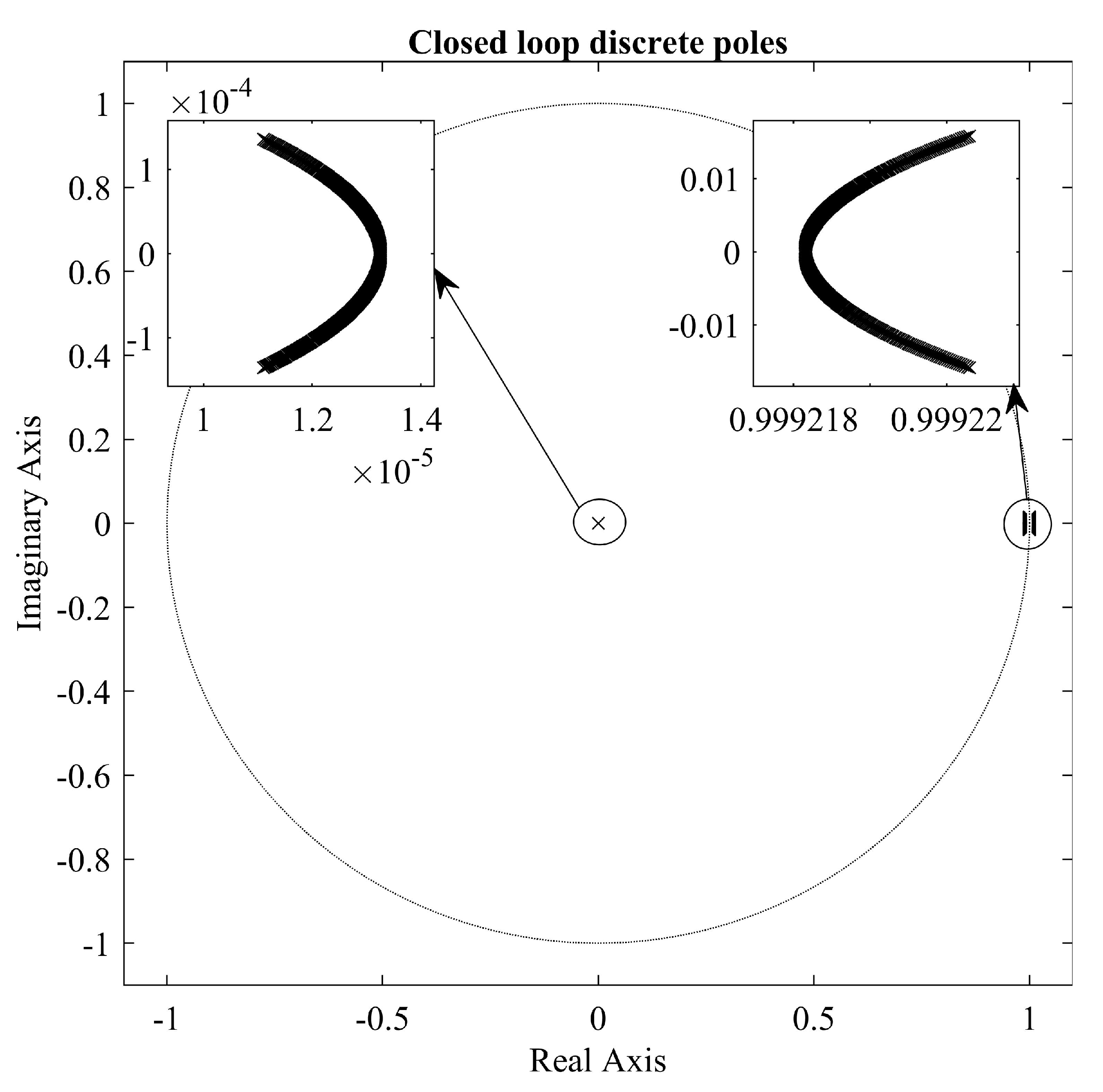
4.1. Stability Analysis

To prove stability of the control law, one must know the closed loop dynamics of the regulated system. The control law (17) derived in the previous section can be plugged into (13) so that closed loop system dynamics can be derived as shown in Equation (24):

$$\begin{array}{c}\hfill \begin{array}{c}\mathit{x}[k+1]={\mathit{A}}^{\prime }\left({\omega }_r\right)\mathit{x}\left[k\right]+{\mathit{B}}_d{\mathit{E}}_d{\mathit{i}}_{\alpha \beta }^{*}[k+1]\\ {\mathit{A}}^{\prime }\left({\omega }_r\right)={\mathit{A}}_d\left({\omega }_r\right)+{\mathit{B}}_d{\mathit{K}}_d\left({\omega }_r\right)\end{array}\end{array}$$

(24)

One can observe that derived control law and closed loop dynamic system resemble classic state feedback control method, where ${\mathit{K}}_d\left({\omega }_r\right)$ can be considered as feedback gain matrix. If the term ${\mathit{A}}^{\prime }$ can be proven to be Hurwitz, i.e., all eigenvalues of the ${\mathit{A}}^{\prime }$ matrix lie in the unit circle, the system can be considered stable. In this case, state matrix ${\mathit{A}}_d\left({\omega }_r\right)$ and feedback gain matrix ${\mathit{K}}_d\left({\omega }_r\right)$ depend on the instantaneous value of the rotor speed ${\omega }_r$, and the expressions for the calculation and analytical representation of eigenvalues of such system become extremely complicated. Therefore, the authors conducted numerical solutions of the system poles for the range of the possible rotor speed values, and graphically presented the poles. This kind of approach was not considered in the referenced papers that deal with similar topics. In [27,28] only the performance is presented, in [29], the stability for the finite control set MPC is achieved by calculating sets of weighing matrices, but no approach for stability of continuous control set MPC. In [30] there is a stability consideration, however the weighing factor calculation is included and discrete Lyapunov function is used.

Figure 2 shows discrete poles of the closed loop system for the rotor speed range: $-157\mathrm{rad}{\mathrm{s}}^{-1}⩽{\omega }_r⩽157\mathrm{rad}{\mathrm{s}}^{-1},{\omega }_r\in \mathbb{Z}$. It can be seen that the closed loop poles stay inside the unit circle throughout the whole speed range, which suggest that the system is stable.

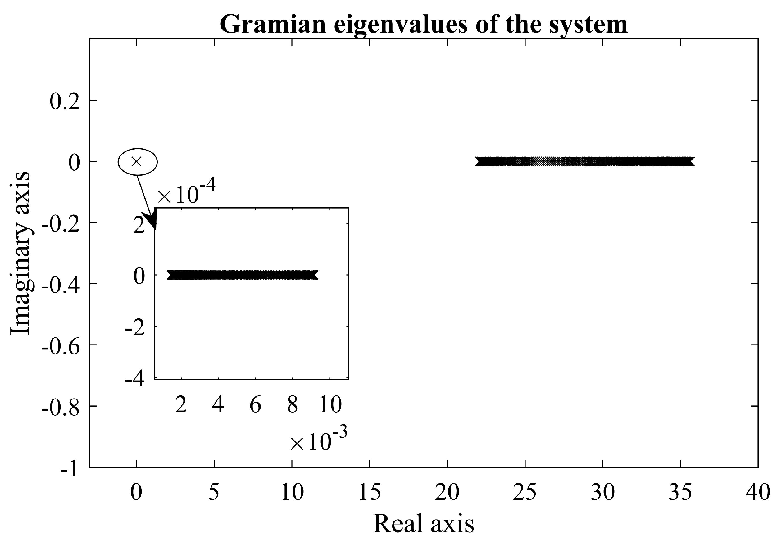
4.2. Controllability Analysis

Since there are parallels that can be drawn between the inner loop regulator and state feedback, it would be interesting to analyze the controllability of the system. This is done by deriving the controllability matrix ($\mathit{Co}$), as shown in Equation (25), and calculating its rank. Like the stability analysis, the procedure will be conducted for the whole range of the possible rotor speed values: $-157\mathrm{rad}{\mathrm{s}}^{-1}⩽{\omega }_r⩽157\mathrm{rad}{\mathrm{s}}^{-1},{\omega }_r\in \mathbb{Z}$.

$$\mathit{Co}=[\mathit{B}\mathit{A}\left({\omega }_r\right)\mathit{B}{\mathit{A}}^2\left({\omega }_r\right)\mathit{B}\dots {\mathit{A}}^{n-1}\left({\omega }_r\right)\mathit{B}]$$

(25)

After calculating the rank of controllability matrix for each rotor speed value, it can be concluded that the system is fully controllable. For better visual representation of the controllability it is convenient to calculate the controllability gramian and plot its eigenvalues. Figure 3 shows the gramian eigenvalues for the aforementioned rotor speed range, and it can be concluded, that since all the eigenvalues have positive real part, gramian matrices are positive definite, which proves the controllability. Further information on the gramian matrix calculation can be found in [34].

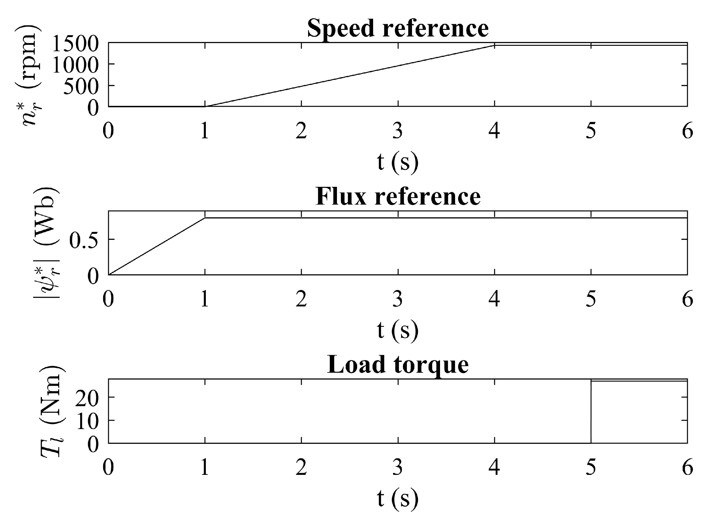
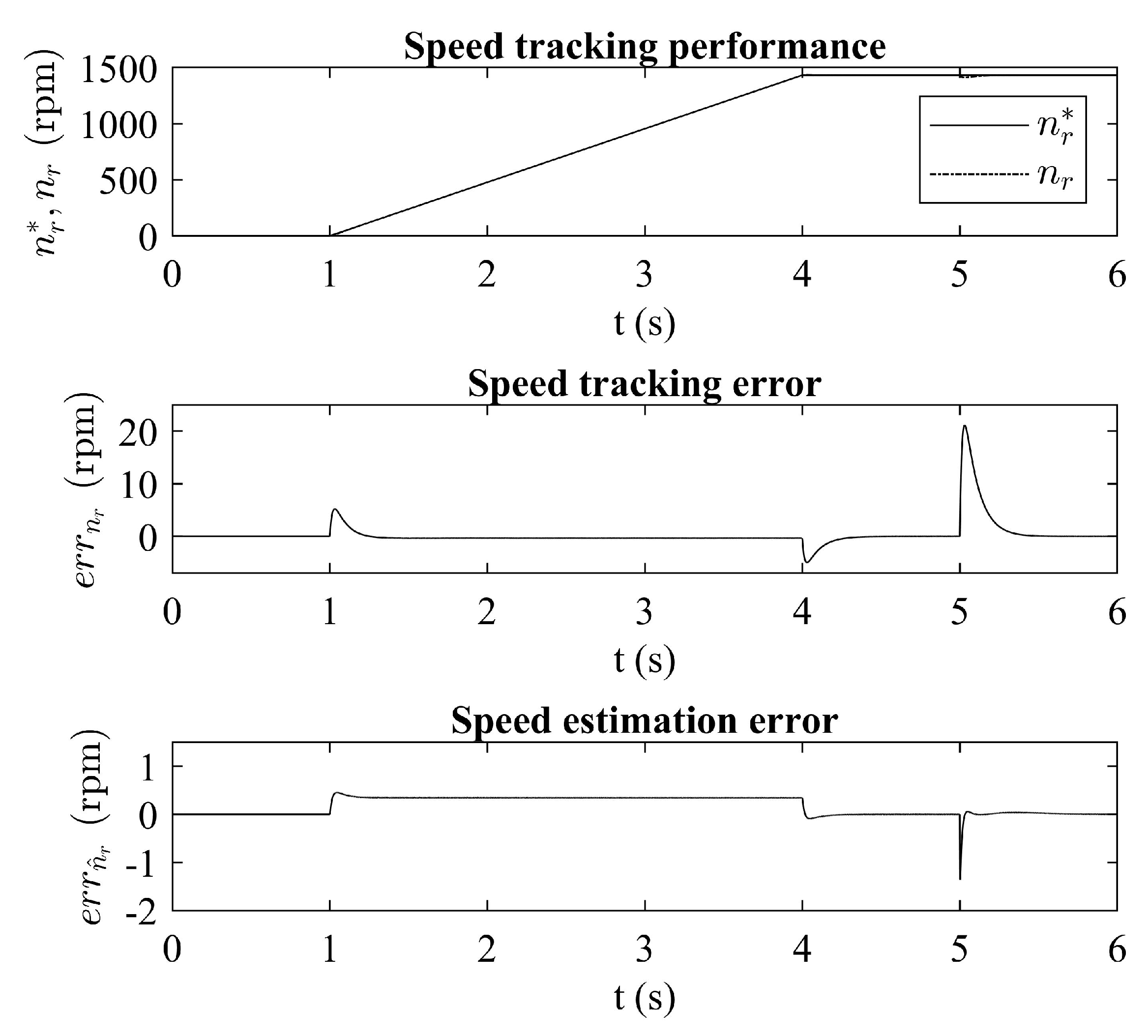
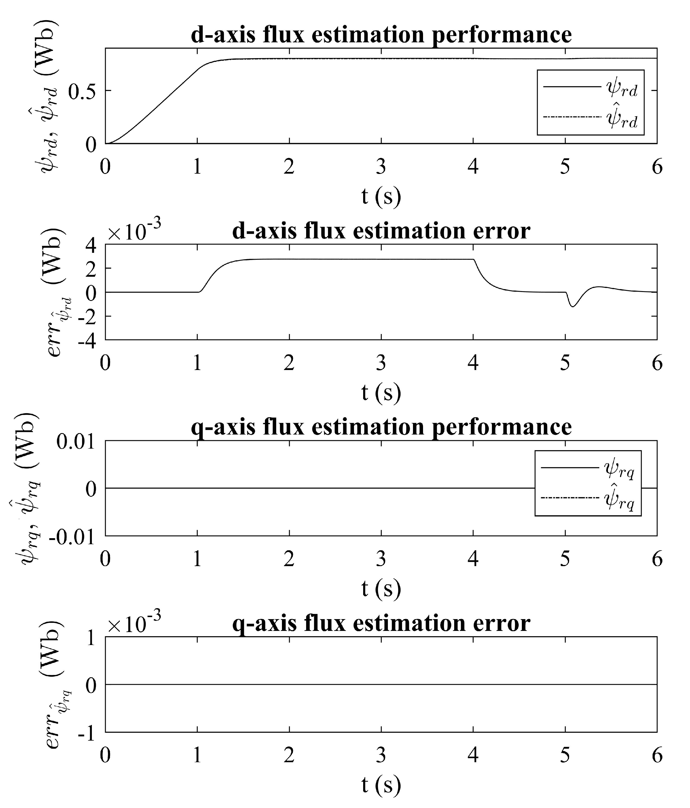
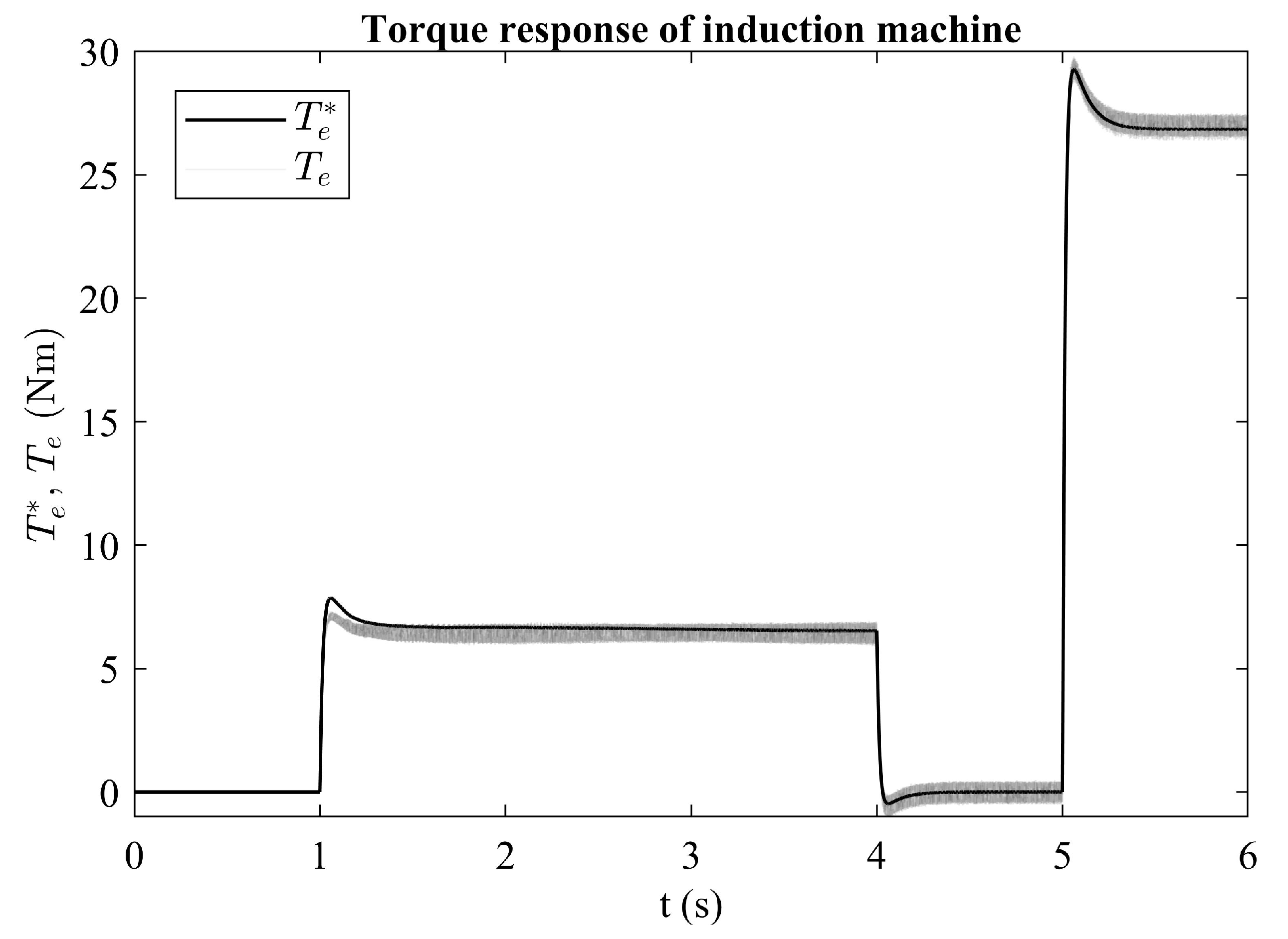
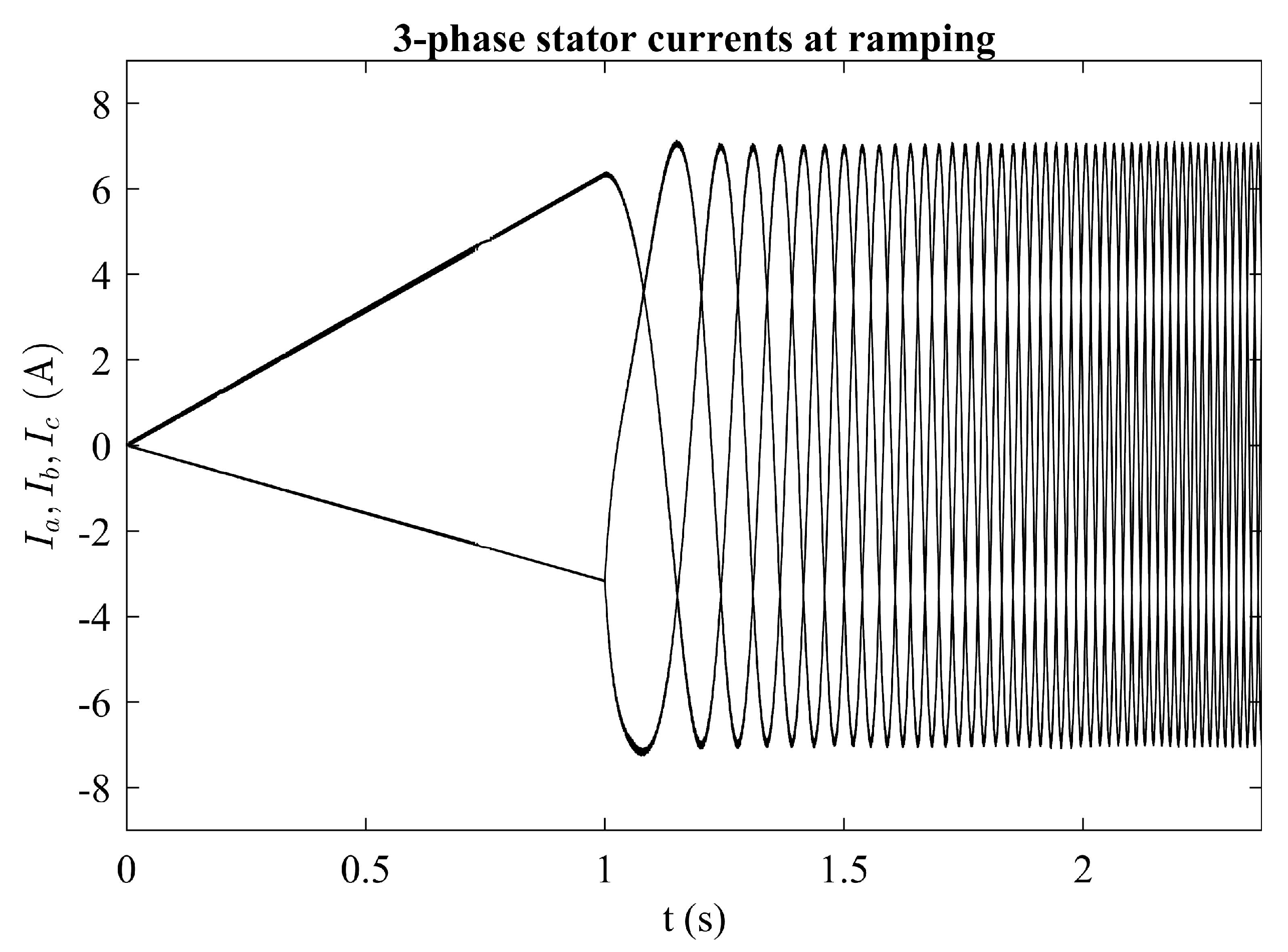
5. Simulation Results

Simulation results will be presented in this section. To simulate the system in more realistic manner, authors implement the inverter and space vector modulator. Inverter model is shown in Equation (26), where $v_{dc}$ represents DC link voltage and ${\mathit{s}}_{1,3,5}={[s_1\hspace{1em}{s}_3\hspace{1em}{s}_5]}^T$ represent the vector of inverter switches that can assume value of zero or one. The information about the implementation of the space vector modulator can be found in papers, such as [35,36]. Modulated DC link voltage (${\mathit{v}}_{\alpha \beta ,mod}$) is then applied to the machine. The simulation is executed in Matlab/Simulink environment and all relevant parameters are shown in Table 1.

$$\begin{array}{c}{\mathit{v}}_{\alpha \beta ,mod}=v_{dc}\left[\begin{array}{ccc}\frac{2}{3}& -\frac{1}{3}& -\frac{1}{3}\\ 0& \frac{1}{\sqrt{3}}& -\frac{1}{\sqrt{3}}\end{array}\right]{\mathit{s}}_{1,3,5}\end{array}$$

(26)

To test the algorithm, following reference signals were applied to the regulator:

• Rotor flux: ramping from 0 to 0.8 Wb during first second of the simulation and stays at the constant value throughout the simulation;
• Rotor speed: ramping from 0 to 1433 rpm during 3 s period, starting from the first second of the simulation and stays at the constant value throughout the simulation;
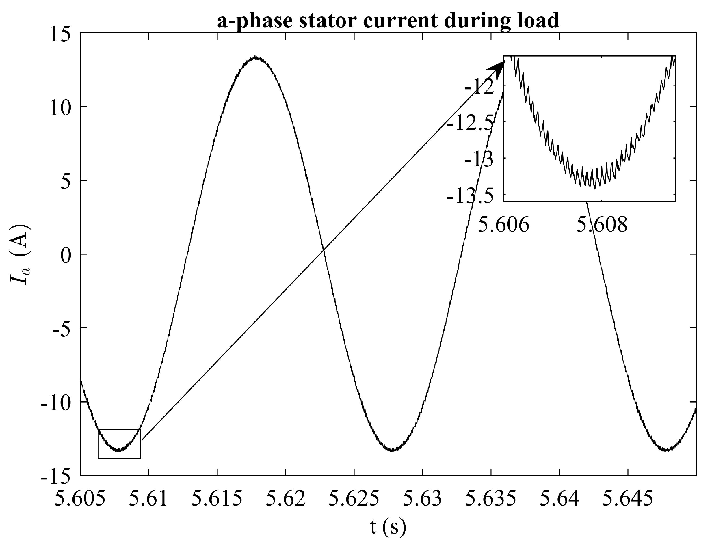
• Load: nominal load torque of 27 $\mathrm{N}\mathrm{m}$ is applied at the fifth second of the simulation and stayed at the constant value throughout the simulation;

Reference signals, along with the load torque are shown in Figure 4.

Figure 5 shows the speed tracking performance of the regulator. it can be seen that the speed tracking error is zero during the steady state, as well as the estimated speed error. During disturbances it can be seen that the error converges to zero fairly quickly.

Figure 6 shows estimated and calculated rotor flux along with the estimation error. Flux components are recalculated into synchronously rotating $dq$-reference frame for better visualization. It can be seen that estimation error is more significant for d-axis component and it is largest during transients, but it converges to zero at the steady state. The amplitude of the largest residual value of d-axis component is only around 0.4% of the total flux value. Estimation error of the flux q-axis component is less significant as it can be seen from the figure.

Figure 7 shows calculated electro-mechanical torque on the machine rotor shaft and torque command generated by the speed PI regulator. It can be seen that the generated torque follows the reference torque, but chattering is clearly visible. This happens because of the switching nature of the regulator, but space vector modulation technique reduces the harmonic content of the chattering.

Chattering is also visible in the stator currents. Figure 8 shows the 3-phase currents at ramping and Figure 9 shows the zoomed in portion of the a-phase current during load period, where the ripple is best seen. As mentioned previously, this unavoidable phenomenon, which can only be reduced but never completely avoided.

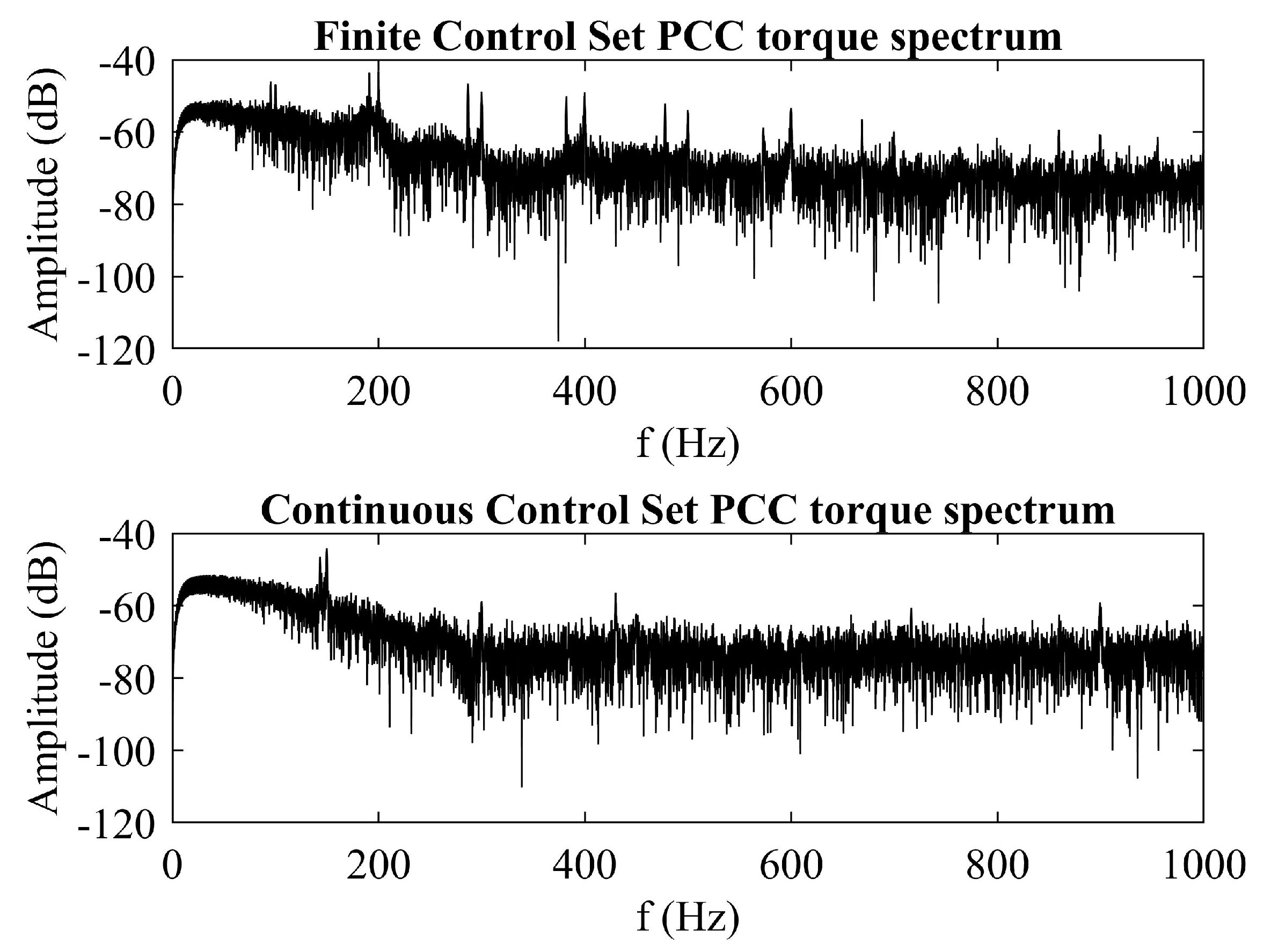
Comparison with Finite Control Set PCC

In this subsection a comparison with the finite control set PCC for induction machine will be conducted. Information about the implementation of finite control set PCC can be found in papers [32] or [11]. Torque responses of both methods were filtered using the lowpass filter to remove the DC torque component. Fourier analysis is then applied to the AC component of the torque and Figure 10 presents the torque harmonic content for the continuous control set PCC, that uses constant switching frequency through means of modulator, and finite control set PCC, that applies optimal voltage vector to the machine each sampling time. It is visible that finite control set PCC has a periodicity of harmonics at each 100 Hz, therefore, higher content of lower harmonics. Both methods show similar amplification of the signal through the frequency spectrum, and higher harmonic content is as expected in variable frequency drives. It is clear that the continuous control set PCC has much lower harmonic content at lower frequencies and exerts less stress on rotor shaft.

6. Discussion

A method for induction machine speed tracking is shown in this paper. The main part of the method is model predictive current control without the need for calculation of the weighing factors for the inner control loop (they are simply set to one). Speed tracking is achieved by simple PI regulator of the outer control loop. Speed and rotor flux estimator is implemented and it is successfully utilized for sensorless control and calculation of the angle for coordinate system transformation. Simulation is carried out, and the method shows great performance during transients and steady state. At the loading instance there is a speed overshoot of 20 rpm (1.4% of reference speed), and around 2 Nm in torque (7% of the reference torque). Additionally, there is improvement compared to the finite control set method, which is visible from frequency spectrum of the generated torque on the rotor shaft. The controllability analysis that was carried out showed that the system is fully controllable, which suggests that pole placement could be conducted and behavior of the system could be manipulated. In the future work, pole placement will be further investigated, along with the experiment that will be conducted on the real time test bench.

References

1. Hasse, K. Zur Dynamik Drehzahlgeregelter Antriebe mit Stromrichtergespeisten Asynchron-Kurzschlusslaaeufermaschinen. Ph.D. Thesis, Technische Hochschule Darmstadt, Darmstadt, Germany, 1969. [Google Scholar]
2. Blaschke, F. Das Verfahren der Feldorientierung zur Regelung der Drehfeldmaschine. Ph.D. Thesis, Eindhoven University of Technology, Eindhoven, The Netherlands, 1973. [Google Scholar]
3. Takahashi, I.; Noguchi, T. A New Quick-Response and High-Efficiency Control Strategy of an Induction Motor. IEEE Trans. Ind. Appl. 1986, IA-22, 820–827. [Google Scholar] [CrossRef]
4. Vazquez, S.; Rodriguez, J.; Rivera, M.; Franquelo, L.G.; Norambuena, M. Model Predictive Control for Power Converters and Drives: Advances and Trends. IEEE Trans. Ind. Electron. 2017, 64, 935–947. [Google Scholar] [CrossRef] [Green Version]
5. Cortes, P.; Kazmierkowski, M.; Kennel, R.; Quevedo, D.; Rodriguez, J. Predictive Control in Power Electronics and Drives. IEEE Trans. Ind. Electron. 2008, 55, 4312–4324. [Google Scholar] [CrossRef]
6. Kouro, S.; Cortes, P.; Vargas, R.; Ammann, U.; Rodriguez, J. Model Predictive Control—A Simple and Powerful Method to Control Power Converters. IEEE Trans. Ind. Electron. 2009, 56, 1826–1838. [Google Scholar] [CrossRef]
7. Rodriguez, J.; Kazmierkowski, M.P.; Espinoza, J.R.; Zanchetta, P.; Abu-Rub, H.; Young, H.A.; Rojas, C.A. State of the Art of Finite Control Set Model Predictive Control in Power Electronics. IEEE Trans. Ind. Inf. 2013, 9, 1003–1016. [Google Scholar] [CrossRef]
8. Wang, F.; Zhang, Z.; Mei, X.; Rodríguez, J.; Kennel, R. Advanced Control Strategies of Induction Machine: Field Oriented Control, Direct Torque Control and Model Predictive Control. Energies 2018, 11, 120. [Google Scholar] [CrossRef] [Green Version]
9. Kennel, R.; Rodriguez, J.; Espinoza, J.; Trincado, M. High performance speed control methods for electrical machines: An assessment. In Proceedings of the 2010 IEEE International Conference on Industrial Technology, Via del Mar, Chile, 14–17 March 2010. [Google Scholar] [CrossRef]
10. Rodriguez, J.; Kennel, R.M.; Espinoza, J.R.; Trincado, M.; Silva, C.A.; Rojas, C.A. High-Performance Control Strategies for Electrical Drives: An Experimental Assessment. IEEE Trans. Ind. Electron. 2012, 59, 812–820. [Google Scholar] [CrossRef]
11. Wang, F.; Li, S.; Mei, X.; Xie, W.; Rodriguez, J.; Kennel, R.M. Model-Based Predictive Direct Control Strategies for Electrical Drives: An Experimental Evaluation of PTC and PCC Methods. IEEE Trans. Ind. Inf. 2015, 11, 671–681. [Google Scholar] [CrossRef]
12. Wang, F.; Chen, Z.; Stolze, P.; Kennel, R.; Trincado, M.; Rodriguez, J. A Comprehensive Study of Direct Torque Control (DTC) and Predictive Torque Control (PTC) for High Performance Electrical Drives. EPE J. 2015, 25, 12–21. [Google Scholar] [CrossRef]
13. Englert, T.; Graichen, K. Nonlinear model predictive torque control and setpoint computation of induction machines for high performance applications. Control Eng. Pract. 2020, 99, 104415. [Google Scholar] [CrossRef]
14. Rojas, C.A.; Rodriguez, J.; Villarroel, F.; Espinoza, J.R.; Silva, C.A.; Trincado, M. Predictive Torque and Flux Control Without Weighting Factors. IEEE Trans. Ind. Electron. 2013, 60, 681–690. [Google Scholar] [CrossRef]
15. Wang, F.; Xie, H.; Chen, Q.; Davari, S.A.; Rodriguez, J.; Kennel, R. Parallel Predictive Torque Control for Induction Machines Without Weighting Factors. IEEE Trans. Power Electron. 2020, 35, 1779–1788. [Google Scholar] [CrossRef]
16. Nemec, M.; Nedeljkovic, D.; Ambrozic, V. Predictive Torque Control of Induction Machines Using Immediate Flux Control. IEEE Trans. Ind. Electron. 2007, 54, 2009–2017. [Google Scholar] [CrossRef]
17. Ahmed, A.A.; Koh, B.K.; Park, H.S.; Lee, K.B.; Lee, Y.I. Finite-Control Set Model Predictive Control Method for Torque Control of Induction Motors Using a State Tracking Cost Index. IEEE Trans. Ind. Electron. 2017, 64, 1916–1928. [Google Scholar] [CrossRef]
18. Zhang, Y.; Xia, B.; Yang, H. Model predictive torque control of induction motor drives with reduced torque ripple. IET Electr. Power Appl. 2015, 9, 595–604. [Google Scholar] [CrossRef]
19. Ouhrouche, M.; Errouissi, R.; Trzynadlowski, A.M.; Tehrani, K.; Benzaioua, A. A Novel Predictive Direct Torque Controller for Induction Motor Drives. IEEE Trans. Ind. Electron. 2016, 63, 5221–5230. [Google Scholar] [CrossRef]
20. Wang, F.; Zhang, Z.; Kennel, R.; Rodríguez, J. Model predictive torque control with an extended prediction horizon for electrical drive systems. Int. J. Control 2014, 88, 1379–1388. [Google Scholar] [CrossRef]
21. Wang, J.; Wang, F. Robust sensorless FCS-PCC control for inverter-based induction machine systems with high-order disturbance compensation. J. Power Electron. 2020, 20, 1222–1231. [Google Scholar] [CrossRef]
22. Wang, J.; Wang, F.; Wang, G.; Li, S.; Yu, L. Generalized Proportional Integral Observer-Based Robust Finite Control Set Predictive Current Control for Induction Motor Systems with Time-Varying Disturbances. IEEE Trans. Ind. Inf. 2018, 14, 4159–4168. [Google Scholar] [CrossRef]
23. Wang, T.; Hu, Y.; Wu, Z.; Ni, K. Low-Switching-Loss Finite Control Set Model Predictive Current Control for IMs Considering Rotor-Related Inductance Mismatch. IEEE Access 2020, 8, 108928–108941. [Google Scholar] [CrossRef]
24. Wang, F.; Wang, J.; Kennel, R.M.; Rodriguez, J. Fast Speed Control of AC Machines without the Proportional-Integral Controller: Using an Extended High-Gain State Observer. IEEE Trans. Power Electron. 2019, 34, 9006–9015. [Google Scholar] [CrossRef]
25. Wang, F.; Zhang, Z.; Wang, J.; Rodríguez, J. Sensorless model-based PCC for induction machine. IET Electr. Power Appl. 2017, 11, 885–892. [Google Scholar] [CrossRef]
26. Vafaie, M.H. Approach for classifying continuous control set-predictive controllers applied in AC motor drives. IET Power Electron. 2020, 13, 1500–1513. [Google Scholar] [CrossRef]
27. Wallscheid, O.; Ngoumtsa, E.F.B. Investigation of Disturbance Observers for Model Predictive Current Control in Electric Drives. IEEE Trans. Power Electron. 2020, 35, 13563–13572. [Google Scholar] [CrossRef]
28. Wróbel, K.; Serkies, P.; Szabat, K. Model Predictive Base Direct Speed Control of Induction Motor Drive—Continuous and Finite Set Approaches. Energies 2020, 13, 1193. [Google Scholar] [CrossRef] [Green Version]
29. Ahmed, A.A.; Koh, B.K.; Lee, Y.I. A Comparison of Finite Control Set and Continuous Control Set Model Predictive Control Schemes for Speed Control of Induction Motors. IEEE Trans. Ind. Inf. 2018, 14, 1334–1346. [Google Scholar] [CrossRef]
30. Ahmed, A.A.; Koh, B.K.; Lee, Y.I. Continuous Control Set-Model Predictive Control for Torque Control of Induction Motors in a Wide Speed Range. Electr. Power Components Syst. 2018, 46, 2142–2158. [Google Scholar] [CrossRef]
31. Krause, P. Analysis of Electric Machinery and Drive Systems; IEEE Press: New York, NY, USA, 2002. [Google Scholar]
32. Rodriguez, J.; Pontt, J.; Silva, C.A.; Correa, P.; Lezana, P.; Cortes, P.; Ammann, U. Predictive Current Control of a Voltage Source Inverter. IEEE Trans. Ind. Electron. 2007, 54, 495–503. [Google Scholar] [CrossRef]
33. Bose, B.K. Modern Power Electronics and AC Drives; Prentice Hall: Hoboken, NJ, USA, 2001. [Google Scholar]
34. Afanasiev, V.N.; Kolmanovskii, V.; Nosov, V.R. Mathematical Theory of Control Systems Design; Springer: Dordrecht, The Netherlands, 1996. [Google Scholar]
35. Ma, Y.; Fan, L.; Miao, Z. Realizing space vector modulation in MATLAB/Simulink and PSCAD. In Proceedings of the 2013 North American Power Symposium (NAPS), Manhattan, KS, USA, 22–24 September 2013. [Google Scholar] [CrossRef]
36. Iqbal, A.; Lamine, A.; Ashraf, I.; Mohibullah. Matlab/Simulink Model of Space Vector PWM for Three-Phase Voltage Source Inverter. In Proceedings of the 41st International Universities Power Engineering Conference, Newcastle upon Tyne, UK, 6–8 September 2006. [Google Scholar] [CrossRef]
Figure 1. Block diagram of the control method.
Applsci 11 06230 g001
Figure 2. Closed loop discrete system poles for range of rotor speed values.
Applsci 11 06230 g002
Figure 3. Gramian eigenvalues for range of rotor speed values.
Applsci 11 06230 g003
Figure 4. Reference and loading signals.
Applsci 11 06230 g004
Figure 5. Speed tracking performance.
Applsci 11 06230 g005
Figure 6. Estimated rotor flux components and estimation errors.
Applsci 11 06230 g006
Figure 7. Commanded and generated torque responses.
Applsci 11 06230 g007
Figure 8. abc-phase stator currents at startup.
Applsci 11 06230 g008
Figure 9. a-phase stator current during load period.
Applsci 11 06230 g009
Figure 10. Fourier analysis of torque for continuous and finite control set PCC.
Applsci 11 06230 g010