Application of Machine Learning to Include Honking Effect in Vehicular Traffic Noise Prediction

Featured Application

Machine learning techniques are calibrated on a dataset of sound levels in urban areas in India, with relevant honking occurrences. The best model chosen will improve the prediction of road traffic noise in similar cases, with respect to standard models that neglect the effects of honking.

Abstract

A vehicular road traffic noise prediction methodology based on machine learning techniques has been presented. The road traffic parameters that have been considered are traffic volume, percentage of heavy vehicles, honking occurrences and the equivalent continuous sound pressure level. L_eq A method to include the honking effect in the traffic noise prediction has been illustrated. The techniques that have been used for the prediction of traffic noise are decision trees, random forests, generalized linear models and artificial neural networks. The results obtained by using these methods have been compared on the basis of mean square error, correlation coefficient, coefficient of determination and accuracy. It has been observed that honking is an important parameter and contributes to the overall traffic noise, especially in congested Indian road traffic conditions. The effects of honking noise on the human health cannot be ignored and it should be included as a parameter in the future traffic noise prediction models.

1. Introduction

The number of vehicles on the roads has been increasing exponentially, both in developing and developed countries. The reasons are consumerism, reduced prices, finance options, competition and the requirement of faster and convenient transport. An inevitable outcome of this continuous production and buying of these vehicles, especially the private ones, has been an increase in the noise and air pollution levels due to the hard traffic congestion, especially in critical areas of the cities [1,2,3]. The effects of air pollution are well known to the general public. To address the problem of environmental pollution, many predictive models and experimental studies have been developed for the traffic management as efficient solution to reduce vehicle journey times and, consequently, environmental impact. For instance, in [4], carbon dioxide (CO₂) emissions and unnecessary fuel consumption are addressed in the framework of route management for autonomous vehicles in urban areas. Conversely, there is a relatively lesser awareness of the harmful effects of traffic noise on the human population. Some of the adverse effects [5,6,7,8] include sleep disturbance, speech interference, annoyance, cardio-vascular effects and loss of fertility. In rare cases, such as with traffic policemen who are exposed to high sound pressure levels and long-term road traffic noise, hearing loss has also been observed [9]. As for the prediction of traffic volumes and the adoption of traffic management strategies to reduce noise pollution levels, a lot of research has been done on the effects of noise on human health [10,11]. Traffic noise prediction models play a very important role not only in the design and modification of road and traffic infrastructure [12] but also in the assessment of the noise level, based on certain critical parameters. Different types of traffic noise prediction models include country or region-specific models like the “Federal Highway Administration model” (FHWA, USA), the “UK Calculation of Road Traffic Noise” (CoRTN, UK), the “Acoustical Society of Japan Road Traffic Noise model” (ASJ, Japan) and the “Richtlinien für den Lärmschutz an Straben” (RLS-90, Germany). A critical review of the most used models can be found in [13,14,15,16]. Other categories of models include static and dynamic, stochastic and deterministic and artificial intelligence or machine learning based models [17,18,19,20,21,22]. In particular, several applications to traffic noise prediction can be found in literature, for instance [23,24,25,26,27], in which the authors adopt artificial intelligence techniques, such as artificial neural networks (ANN) and genetic algorithms (GA).

In most recent studies, hybrid models combining systems of ANN and fuzzy interference systems (FIS) (i.e., adaptive neuro fuzzy inference system—ANFIS) have been developed too [28]. Other hybrid models are represented by the integration between time series analysis techniques and ANN [29].

The different parameters that are generally considered in these models are traffic volume (number of vehicles per unit of time), percentage of heavy vehicles, average speed of vehicles, tyre–road interaction, building height, road width and gradient etc. One parameter that has generally been not considered and is quite prevalent in the Indian road conditions is honking noise.

The relevance of the honking in the Indian scenario has been demonstrated in several studies. In [30], for example, it is reported how the expansion of the transportation industry in the city of Nagpur led to an increment of 5–6 dBA in noise level, 4–6 times in honking and 1.7 times in traffic volume.

The Indian roads traffic conditions are quite different because of the size of the population, topography of the roads, vehicle types and conditions, driving habits and culture. Because of the congested traffic conditions and anxious drivers, the effect of honking on the overall traffic noise and its effects on the drivers, pedestrians, cyclists, traffic police personnel, nearby shopkeepers and residents needs to be considered. In this heterogeneous composition of traffic, horn events get to increase noise level (L_den) up to 0.5–13 dBA compared to homogenous traffic conditions [31]. Therefore, the prediction models used for homogenous traffic conditions are not applicable in this heterogeneous context. Thus, to increase the accuracy of noise prediction models, considering honking is required.

Some models considering honking have been developed by using regression model and statistical analysis [32], others by introducing a factor for horn correction, with respect of level of service (LOS), in traffic noise models such as CRTN, FHWA, and RLS 90 [31].

In the present work, an attempt has been made to include the honking effect in the traffic noise prediction model developed using machine learning methods. In particular, four different techniques have been selected, calibrated and tested on a case study experimental dataset collected in Patiala city, India. A comparison of these techniques on the basis of criteria of mean square error, correlation coefficient, coefficient of determination and accuracy has also been presented.

2. Materials and Methods

2.1. Dataset and Sites Description

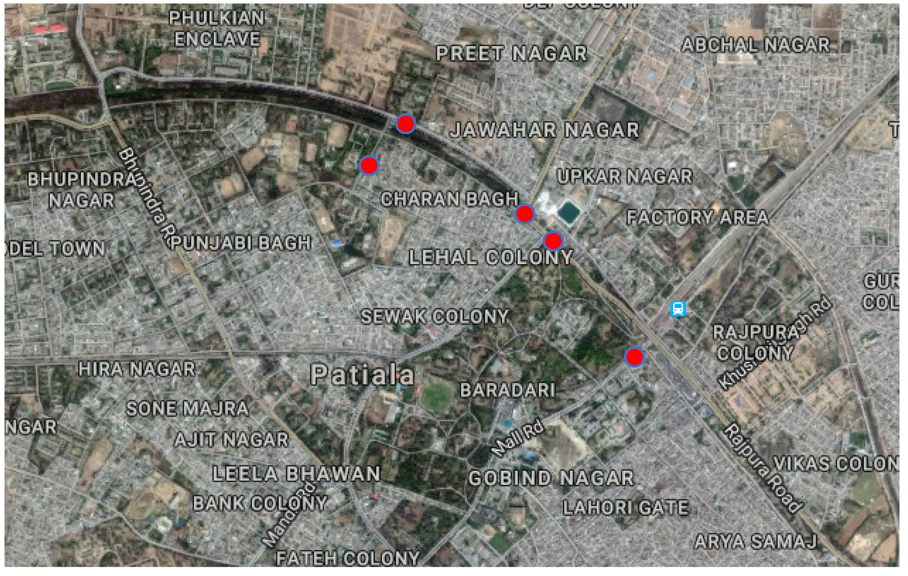
The data used in this paper has been collected on the busy urban roads of the Patiala city in India (Figure 1). Besides the equivalent continuous sound pressure level (L_eq), the data collection included the parameters traffic volume (Q), percentage of heavy vehicles (P) and total honking occurrences (H) that have been used to calibrate and test the machine learning models. These parameters have been collected manually using videography at five different identified sites, highlighted in Figure 1, on the basis of congestion, presence of honking noise and proximity to resident population. For each video, the numbers of light and heavy vehicles have been annotated, as well as the number of honks in each 15 min measurement.

In order to include the effect of horn noise in the prediction model, the number of honking events per 15 min was recorded. The values of the equivalent sound pressure level (L_eq in dBA) have been experimentally measured using a sound level meter (SLM, B&K make, 2250). The sound level meter used was a class 1 integrating type, which meets with the IEC specifications (IEC 61672-1: 2002, International Electrotechnical Commission, 2002) [33]. The SLM was mounted on a tripod (in order to avoid the human body impedance effects), at a height of 1.2 m above the ground level [34] and at a distance of 1 m from the edge of the road where the traffic noise measurements were taken.

A brief description of the sites is given below.

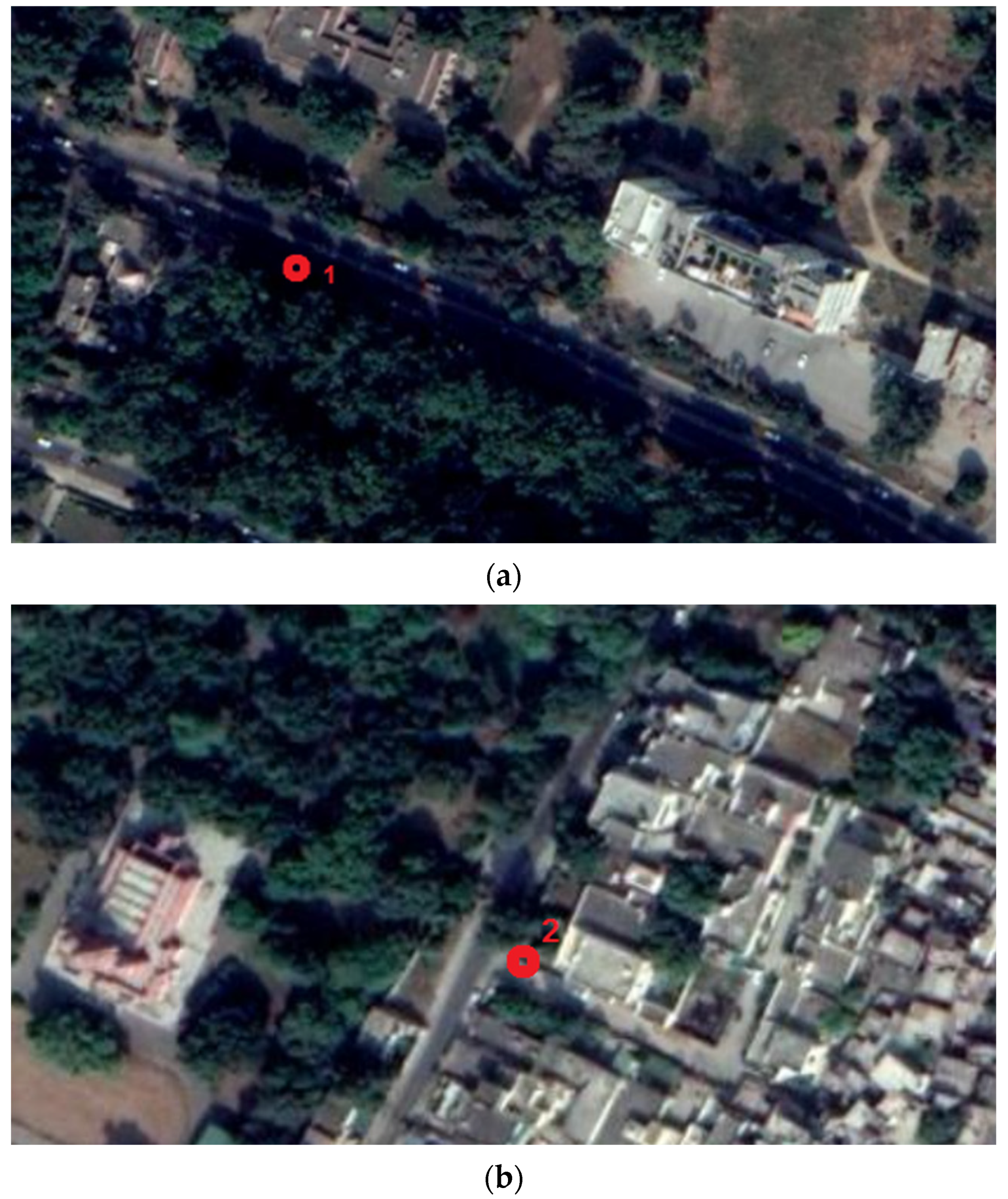
Site 1: This site is located near the Hanumaan Temple, on the road connecting the Mini-secretariat and Gurudwara (a Sikh temple) Dukhniwaran Sahib (Figure 2a). The road has one-way traffic with a median/divider in the middle. The traffic is free-flowing with all types of vehicles plying on the road. There are no traffic lights or a roundabout near the measurement point. The noise generation is mainly due to the vehicle noise and tyre–road interaction noise. There is a thick belt of trees on one side of the road, which leads to noise attenuation by absorption due to the thick foliage.

Site 2: The site consists of a two-way road near the Modi Temple, connecting the Passy road to the State College road (Figure 2b). There is free-flowing traffic, with mainly cars and two-wheelers, and no traffic congestion. On one side, there is open land of the Modi temple ground with some sparse trees and boundary wall. Thus, there is some noise attenuation happening due to air-absorption. On the other side there are residential houses, mostly double storied, that may provide some noise attenuation.

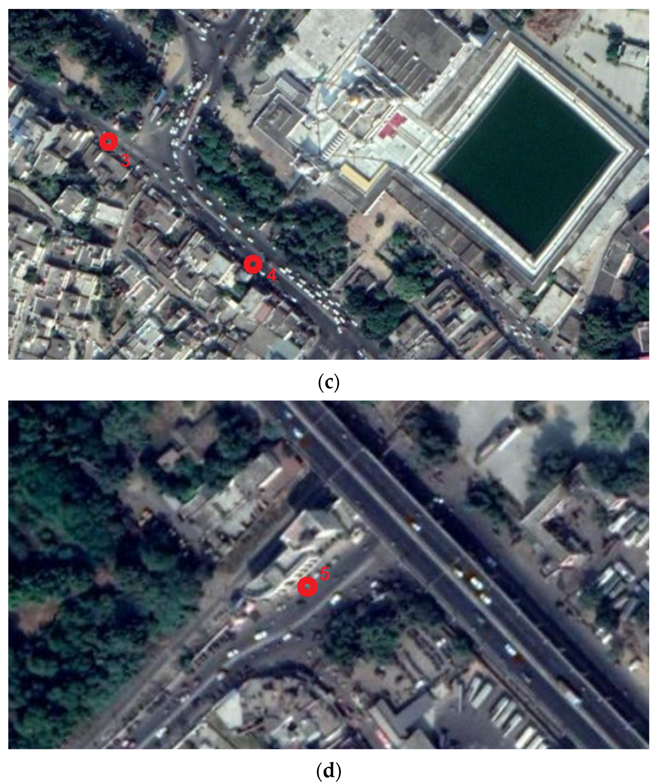
Site 3: It consists of the road connecting the Gurudwara Dukhniwaran Sahib with the Passy road (Figure 2c). The speed of the vehicles is low here because of a narrow section through which the vehicles enter and also because of some fruit stalls and shops nearby. Due to the low speed and some congestion, more honking events have been observed.

Site 4: It is located on the road in front of the main entrance of Gurudwara Dukhniwaran Sahib (Figure 2c). The road is a one-way road with a median/divider in the middle. The traffic volume is very high as the vehicles arrive from different sections of the city and converge here to pass through this bottle-neck section and then go to Mini-secretariat road or the Sirhind road. There is a large number of heavy vehicles passing through this section as the vehicles coming from bus stand or other areas move out of the city using this road, to reach the Sirhind road and then subsequently to the national highway. On one side there is the Gurudwara Sahib main premises and the outer boundary wall, and on the other side, there are shops. High traffic noise levels are observed here due to the large traffic volume as well as honking.

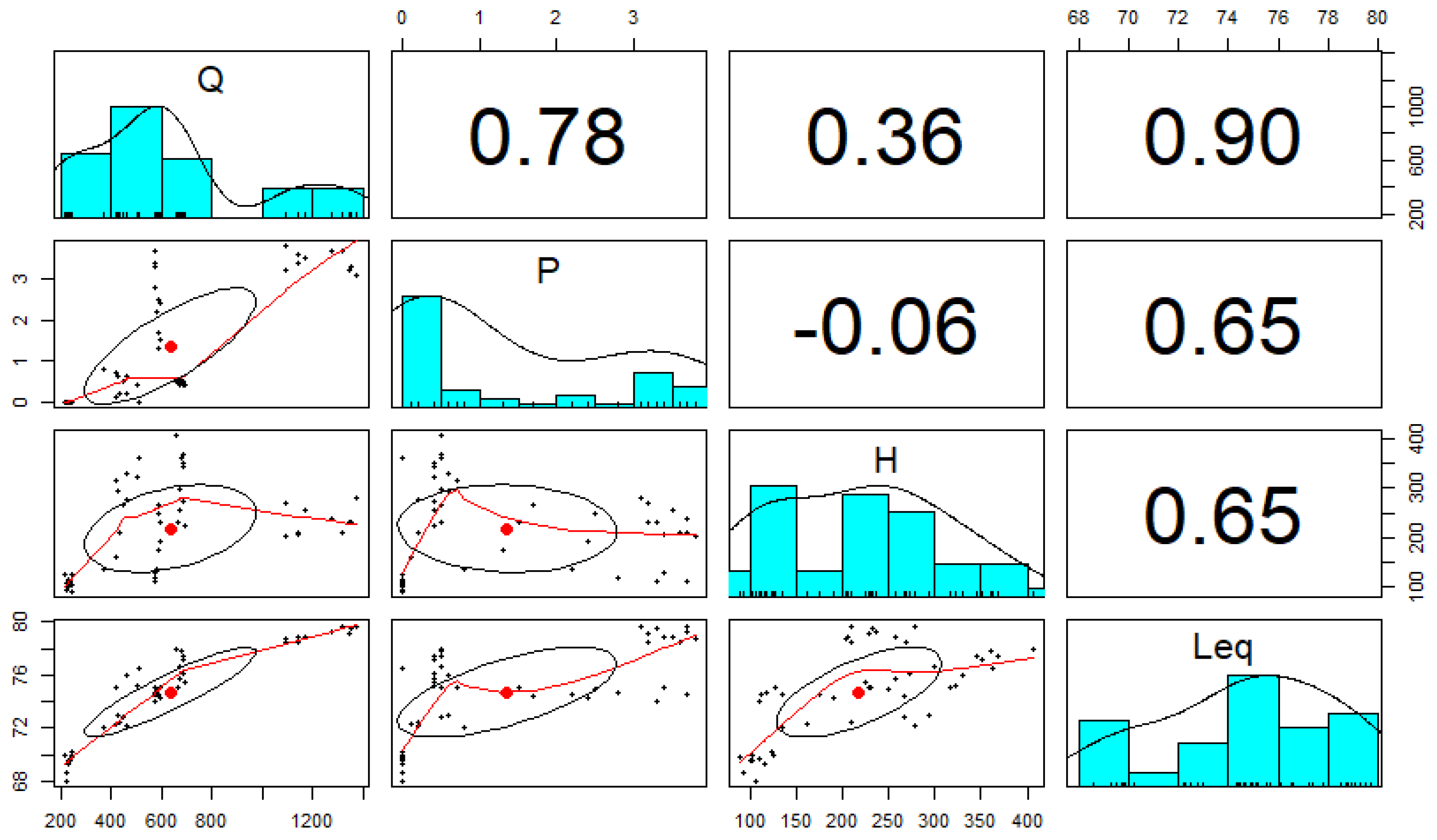
Site 5: The site is situated near the Patiala Bus stand (Figure 2d). A lot of cars, two wheelers and three wheelers pass through this section. The speed of the vehicles is low due to the traffic congestion, as people come here to pick and drop passengers at the bus stand. This also leads to the highest number of horns/honking events observed here giving rise to high noise levels.

A description of the data collected at the above sites, with some statistical analysis and insights into the same is presented below.

The data was collected for 10 days at each site, with 15 min time span, so a dataset of 50 days has been obtained for all the five sites. A resume of the data main statistics is reported in

Table 1. Resume of the main statistics of data and parameters used in the calibration and testing of the models. All the features have been measured with 15 min time span.

	Mean	Standard Deviation	Median	Min	Max
Traffic volume in 15 min (Q) [veh]	633.8	341.2	583	216	1377
Percentage of heavy vehicles (P) [%]	1.36	1.42	0.5	0	3.8
Total honking occurrences in 15 min (H) [counts]	218.0	88.9	227	90	406
Equivalent continuous sound level (Leq) [dBA]	74.7	3.4	75	68	79.7

, while the full dataset is reported in Appendix A.

2.2. Bivariate Correlation Analysis

A bivariate correlation analysis has been performed in R software framework [35]. Results are reported in Figure 3, in which traffic volume (Q), heavy vehicle percentage (P), total honking occurrences (H) and measured equivalent continuous sound pressure level (L_eq) are reported with bivariate scatter plots below the diagonal, histograms on the diagonal and the Pearson correlation above the diagonal. A high correlation (0.90) is found between L_eq and traffic volume, as expected since the main noise sources in the measurement sites are the vehicles. A significant (0.65) correlation is found between L_eq and P, as well as between L_eq and H.

It is interesting to notice that the heavy vehicle percentage, that is usually implemented in the most common road traffic noise models, being recognized as an important parameter of the phenomenon, correlates with the noise levels similarly to the total honking occurrences, that is practically always neglected. In the authors’ opinions, this means that, at least in the five test sites and in all the sites with similar features, the honking events cannot be ignored when designing and calibrating an effective traffic noise model.

2.3. Machine Learning Methodologies

The traffic noise prediction models were developed using four machine learning methods in R software [35], namely decision trees (DT), random forests (RF) [36], generalized linear models (GLM) and artificial neural networks (ANN) [24,25]. These methods have been implemented in the ‘Rattle’ (R) software [37] which is open source and has a GNU (general public license).

The different machine learning methodologies used in the present work are briefly described below:

(i).

Decision Trees (DT) [18]: These methodologies are employed in machine learning applications where an analysis of the data is required. They use a structure which resembles a flow chart as they are based on deterministic data structures and used in classification problems. At the top of the tree, there is a root node and the branches represent the tests that are done and the leaves denote the results of the tests. The rpart( ) function builds a decision tree model. A decision tree works by splitting nodes into sub-nodes. The parameter MinSplit describes the minimum number of members that a node should have before the split is attempted. MaxDepth indicates the maximum depth or length of the tree, starting from the root node up to the leaf node. MinBucket parameter specifies the minimum number of entities that a leaf node can have. The default value is generally one-thirds of the MinSplit value.

(ii).

Random Forests (RF) [36]: In this approach, groups of decision trees are created. This is an ensemble method, which can be used for regression, classification and other tasks. They avoid over-fitting, which can be a drawback in the decision tree method, by making random decision forests. The observations are used as input for each tree and the most common outcome is used as the final output. As the errors are cancelled out, a more accurate prediction is obtained using this method. The randomForest( ) function is used for the implementation of the random forests. Breiman (2001) [36] introduced the idea of random sampling of variables at each node as the tree is being built. He also introduced the bagging concept for the sampling [38] in which random samples are chosen for the training dataset for each tree. It helps in making the model robust to noise and outliers. The parameter ntree specifies the number of trees built in the Random Forests model.

(iii).

Linear Models: Generalized linear models (GLM) make use of and combine different types of regression, e.g., linear and logarithmic [39]. They take care of different types of distribution like the log-linear and log-odds, as the response is not always linear and might not follow a normal distribution.

(iv).

Neural Networks [40]: Artificial neural networks (ANN) are similar in working to the human brain which uses neurons (connections of nodes) for the learning tasks. The process involves the assignment of weights to the inputs and activation functions for getting the desired outputs. There are different layers in a neural network like an input layer, a hidden layer (which performs non-linear transformations of the inputs) and an output layer of neurons. The function neuralnet( ) is used to build a neural network model in R software [35]. The parameter hlayers is used to specify the number of hidden layer nodes or neurons in the NN architecture. MaxNWts sets the maximum limit of the number of weights that can be used in the model. The maxit parameter defines the maximum number of iterations to be done during the training.

The values of the training hyperparameters for the different methods have been taken based on experience and literature survey and are briefly given below.

For the decision trees, the value of MinSplit used is 20, MaxDepth 30 and MinBucket 7. The type of random forest used in RF is regression. The number of trees is 500 and the number of variables tried at each split is 1. The sampling type is bagging. In the neural networks, the number of hidden layer nodes or neurons is 10 with one hidden layer, epochs 150 and the batch size is 8. The activation function used is Sigmoid, dropout rate is 0.2, number of units is 30 and the learning rate is 0.01. The optimizer used is Grid Search. Some of the values, along with names of modules, are given in

Table 2. Machine Learning Methods Used [41].

Model	Method	Name of Module	Input Parameters and Values
Decision Trees	rpart	Rpart	MinSplit = 20, MaxDepth = 30, MinBucket = 7
Random Forests	rf	randomForest	ntree = 500, sampling = bagging
Linear Models	lm	glm	None
Neural Networks	neuralnet	Neuralnet	hlayers = 10, MaxNWts = 10,000, maxit = 100

.

2.4. Perfomance Metrics

The results obtained by using the methods described above were compared on the basis of the criteria of correlation coefficient (r), coefficient of determination (R²), mean square error (MSE) and accuracy, briefly resumed in this subsection.

2.4.1. Correlation Coefficient (r)

The correlation coefficient (r) is a measure of a linear correlation between two sets of data. In particular, it measures the closeness of the points in a scatter plot to the linear regression obtained on the basis of the input data. This parameter can be evaluated as follows [42]:

$$\mathrm{r}=\frac{\mathit{Cov} (X,Y)}{\sqrt{s_x^2{s}_y^2}}$$

(1)

where $Cov \left(X,Y\right)$ is the covariance and $s_x^2$ and $s_y^2$ are the sample variance for X and Y. Obviously, a coefficient of correlation close to 1 indicates a strong linear correlation while a coefficient r close to 0 suggests a little correlation between the investigated parameters.

2.4.2. Coefficient of Determination (R²)

The coefficient of determination R² provides the percentage variation in Y explained by X-variable. It is the square of the coefficient of correlation (r) therefore it is a measurement used to explain how much variability of one factor can be caused by its relationship to another related factor. When the coefficient of determination is equal to 1, the regression line fits all the sample data [42].

2.4.3. Mean Squared Error (MSE)

MSE is a measure of the difference between the measured and the predicted values. It is a sample standard deviation of the differences between the observed values and those predicted by the model. These are called residuals when the differences are calculated for the sample (called in-sample) points, that were used to make the model and prediction errors when the calculations are done for out-of-sample data points. It is calculated as [42]:

$$\mathrm{MSE}=\frac{{\sum }_{i=1}^n{\left(b_i{-a}_i\right)}^2}{n}$$

(2)

where, a is the observed value, b is the predicted value and n is the number of sample data points.

2.4.4. Accuracy

The accuracy is defined in percentage as the mean of the number of the differences between the predicted and the observed values of the dependent variable, that fall within a given range e (i.e., within an acceptable error) [28,41]. It can be calculated as follows:

$$\begin{array}{c}\mathrm{Acc}=\frac{100}{n}{\displaystyle {\displaystyle \sum }_{i=1}^n}{c}_i\\ c_i=\{\begin{array}{l}1,\hspace{1em}\mathrm{if} \mathrm{abs}\left(b_i{-a}_i\right) \le e\\ 0,\hspace{1em}\mathrm{otherwise}\end{array}\end{array}$$

(3)

where, b is the predicted value of dependent variable, a is the observed value of dependent variable, e is the acceptable value of error and n is the total number of samples.

The results obtained are presented in the subsequent section.

3. Results and Model Comparison

The results obtained by using the four machine learning models are compared on the basis of r, R², MSE and accuracy. The above relation has been used for an accuracy of ±1 dBA. The values of the different criteria for the four models are shown in

Table 3. Comparison of results for the prediction models in the training phase.

Machine Learning Method	r	R2	MSE [dBA]	Accuracy (±1 dBA) [%]
Decision Trees (DT)	0.935	0.876	0.884	68
Random Forests (RF)	0.987	0.975	0.413	94
Generalized Linear Model (GLM)	0.974	0.949	0.616	82
Neural Networks (ANN)	0.974	0.949	0.616	82

.

It is seen that random forests performs better than other models in the training phase, in the criteria of r, R², MSE and accuracy. The value of MSE is 0.413 for rf which is the lowest and the value of accuracy is 94% (for ±1 dBA) which is the highest among all other models.

However, for a proper comparison, a testing dataset check was performed, in order to avoid overfitting.

In order to meet this objective, the dataset was split into 70/30 as training and testing data, respectively. Following the training, using the 70% data, the models were tested on the testing dataset (30%). This was done 10 times (ten-fold cross validation) for the best performing model in order to check the stability and robustness of the model. The results obtained from the testing dataset show that the generalized linear model (GLM) performs better on the considered criteria, as seen in the

Table 4. Comparison of results for the prediction models (testing dataset).

Machine Learning Method	r	R2	MSE [dBA]	Accuracy (±1.0 dBA) [%]
Decision Trees (DT)	0.797	0.636	1.780	40.0
Random Forests (RF)	0.955	0.913	0.797	60.0
Generalized Linear Model (GLM)	0.965	0.933	0.666	80.0
Neural Networks (ANN)	0.959	0.921	0.717	73.3

.

As seen in Table 4, the value of mean square error is the lowest (0.666) for the generalized linear model (GLM) and the accuracy is highest (80.0%). The values of MSE and accuracy obtained with neural networks are 0.717 and 73.3% respectively. Random forests and neural networks might give better results for bigger datasets but for the present case, GLM has outperformed the other models.

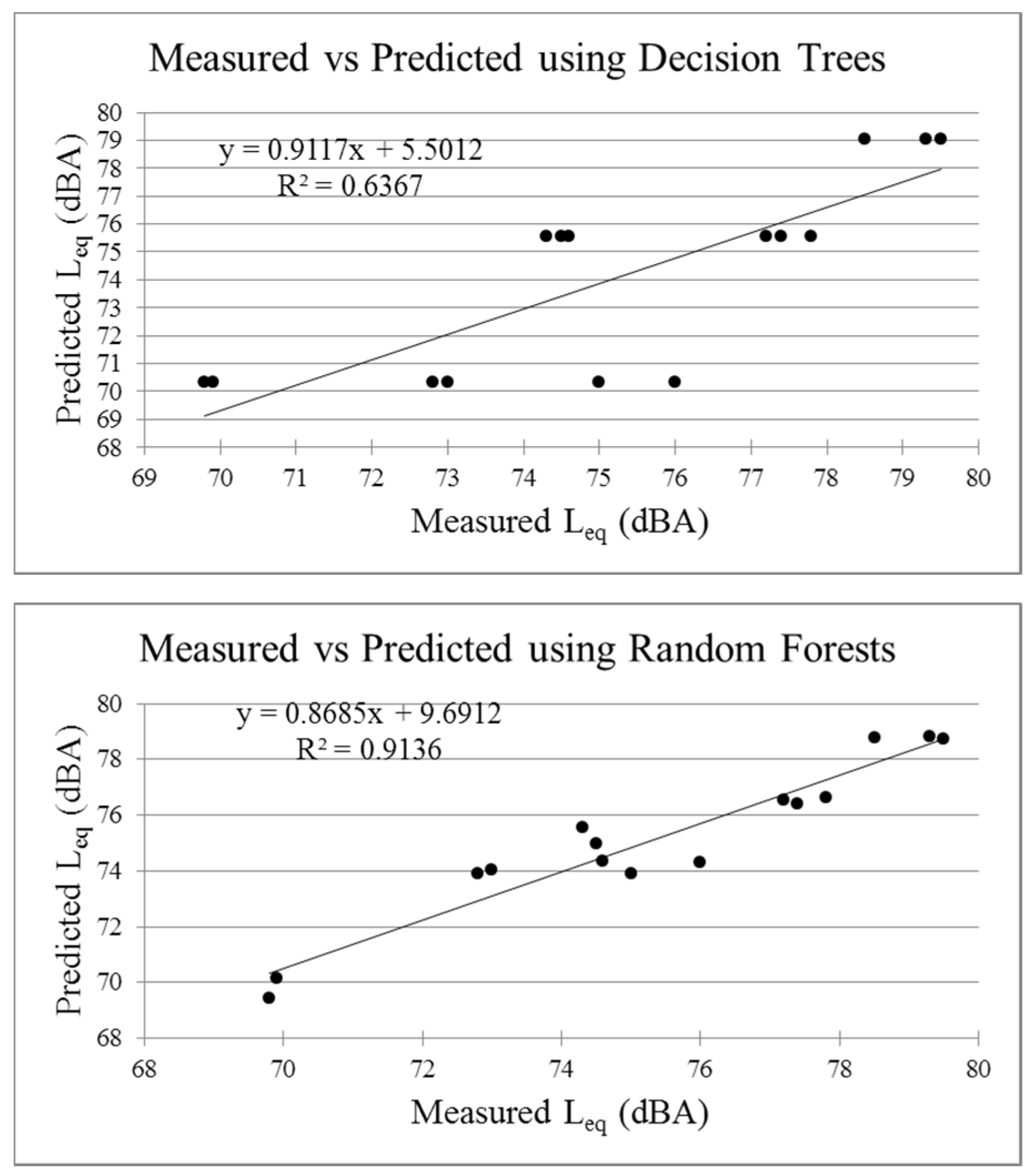
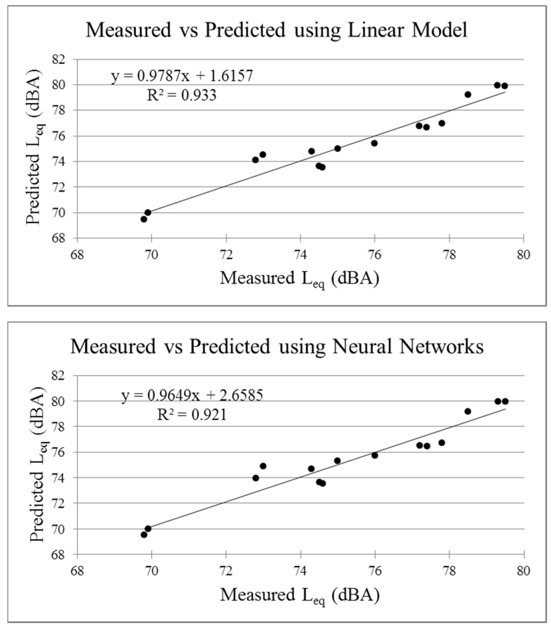
Results of the models’ predictions plotted versus measured equivalent levels in the validation and training datasets are shown in Figure 4. It is easy to see that apart from decision trees (DT) that in 4 points is very far from the measured L_eq, all the models’ results are gathered almost close to the bisector, meaning a general effectiveness of the proposed models. When the measured L_eq are around 70 dBA (site 2), the models have the best performances. This site is characterized by absence of heavy vehicles and honking frequencies lower than in the other sites. Data above 78 dBA are related to site 4, in which the traffic flows are higher than in the other sites.

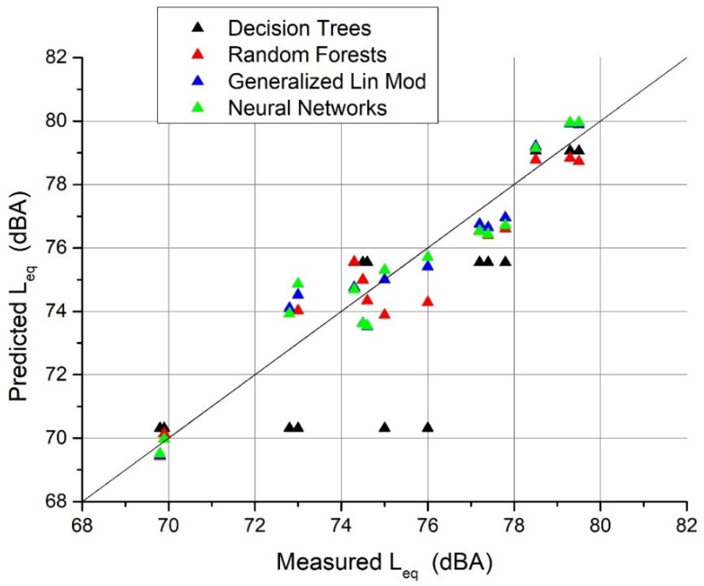
A scatter plot between the measured and predicted values of L_eq for the four methods is shown in Figure 5.

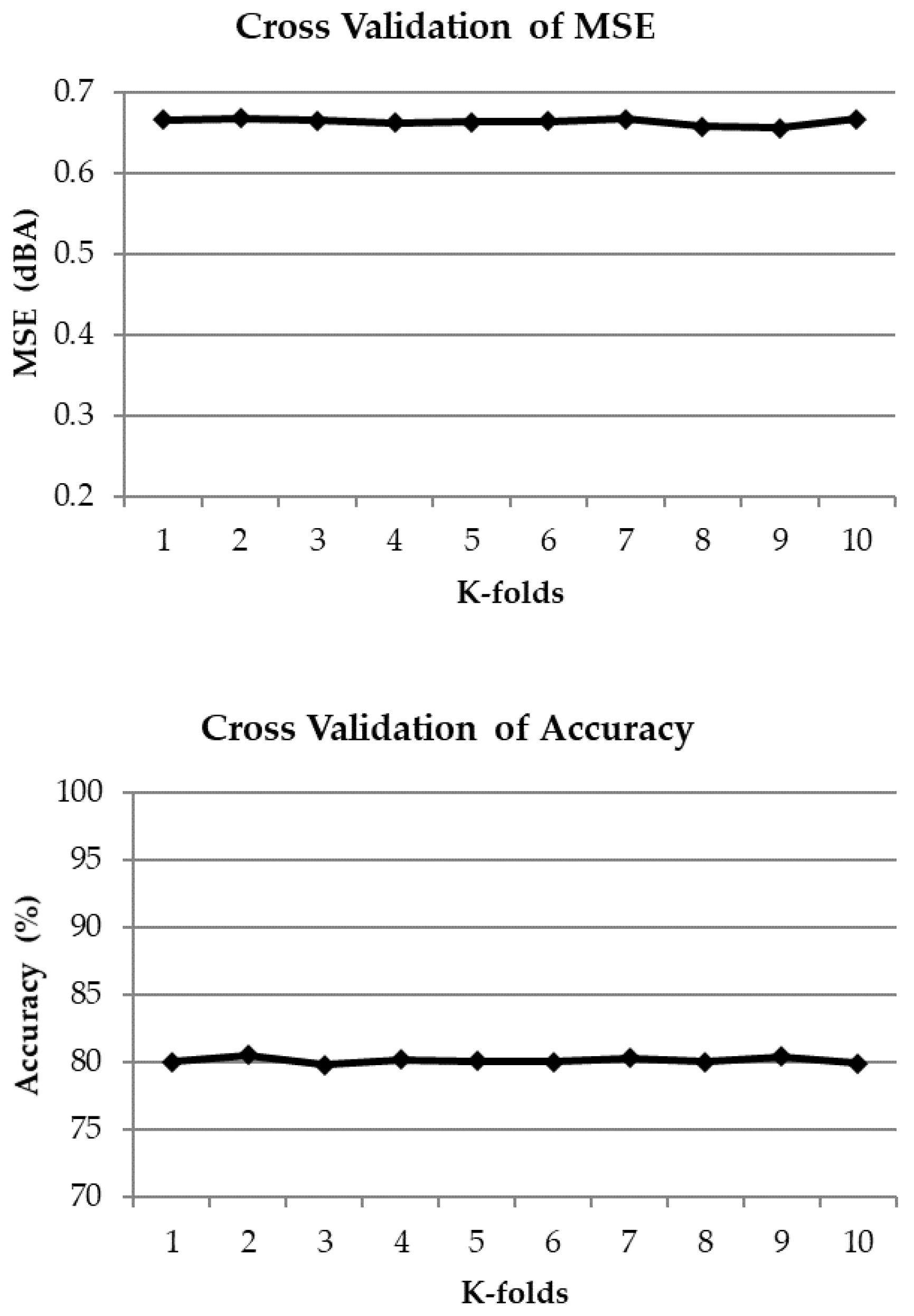
A ten-fold cross validation was also performed for the best performing model, GLM and the results are shown in Figure 6. A general stability of the results is observed, confirming the goodness of the model and the suitability to be used in such applications, on noise data that includes a relevant contribution from honking.

4. Discussion

The results reported in Section 3 inspire interesting discussions and allow to draw some preliminary conclusions.

Looking at the scatter plot reported in Figure 4, it is easy to see that, apart from decision trees (DT), some points underestimate the measured L_eq and all the models’ results are gathered almost close to the bisector, meaning a general effectiveness of the proposed models. When the measured values of L_eq are around 70 dBA (site 2), the models have the best performance. This site is characterized by the absence of heavy vehicles and honking occurrences lower than in the other sites.

Data above 78 dBA are also associated with good performances of the models. These points are related to site 4, in which the traffic volumes are higher than in the other sites.

Finally, the larger dispersion is observed in the middle range of noise levels. In this range basically all the models produce results that are different with respect to the observed noise levels. There is not a clear pattern of overestimation or underestimation, meaning that these errors are basically random for all the models. Only the data comprised in the range 77–78 dBA seems to show a general underestimation of the models. These points belong to site 5, in which the highest mean honking occurrences has been observed.

In order to highlight the importance of the honking inclusion in the models, a simulation without the honking parameter has been performed on the same dataset, both in training and testing phases. Results of the performance metrics without honking are reported in

Table 5. Comparison of results for the prediction models in the training phase (without considering honking).

Machine Learning Method	r	R2	MSE [dBA]	Accuracy (±1 dBA) [%]
Decision Trees (DT)	0.933	0.871	0.902	64
Random Forests (RF)	0.978	0.957	0.526	82
Generalized Linear Model (GLM)	0.904	0.818	1.182	40
Neural Networks (ANN)	0.904	0.818	1.182	40

and

Table 6. Comparison of results for the prediction models (testing dataset) without considering honking.

Machine Learning method	r	R2	MSE [dBA]	Accuracy (±1.0 dBA) [%]
Decision Trees (DT)	0.798	0.637	1.781	40.0
Random Forests (RF)	0.955	0.913	0.809	66.7
Generalized Linear Model (GLM)	0.880	0.774	1.291	46.7
Neural Networks (ANN)	0.880	0.774	1.291	46.7

.

Comparing with results reported in Table 3 and Table 4, it can be noticed that the inclusion of honking in the modeling leads to an overall improvement of the performance metrics. The DT model seems to be not sensible to honking, since the metrics are basically constant with and without honking inclusion, both in training and testing phases. RF in testing dataset keeps r and R² basically constant, the accuracy has a little increase from 60.0% to 66.7%, but MSE increases from 0.797 dBA to 0.809 dBA. The other two models, namely GLM and ANN, converge to similar predictions and, consequently, to equal performance metrics. They exhibit a worsening of all the selected metrics when honking is not considered. Since GLM was the best performing model in the training dataset with honking, it is evident that the inclusion of this parameter leads to a better prediction of noise levels in the presented application. When honking is not included, the MSE of GLM increases from 0.666 dBA to 1.291 dBA and the GLM accuracy gets worse, lowering from 80% to 46.7%.

Regarding the cross validation of GLM, the ten-fold cross validation results reported in Figure 6 shows a general stability. This confirms the goodness of the model and the suitability to be used in such applications, on noise data that includes a relevant contribution from honking.

Although the dataset is sufficient for the present study, a bigger dataset with a greater spread across different times of the year and more sites can be prepared and utilized in a future study. A limitation of the present study, in fact, is that the models are region-specific, since they are based on the data collected at the specific sites identified for the assessment.

The number of input parameters is limited to three in the present work (i.e., traffic volume Q, percentage of heavy vehicles P and total honking occurrences H). In a future work, this number can be expanded including more parameters like speed of vehicles, different types of vehicles (e.g., two-wheelers, three-wheelers etc.) and acceleration-deceleration of vehicles, etc. Furthermore, an assessment of the actual increase in the noise level (in dBA) due to honking can be made and the effect of the duration of the different types of horns used on different vehicles needs to be studied.

5. Conclusions

A traffic noise prediction approach using machine learning methods has been presented, which considers the parameter of honking noise. Horn noise contributes significantly to the overall road traffic noise in Indian road traffic conditions as well as other regions in the Indian sub-continent. Therefore, there is a need to pay attention to this important parameter while developing traffic noise models. An approach to include the effect of honking noise by considering the honking occurrences as a parameter has been illustrated with the help of a case study of the Patiala city in India. A preliminary multivariate analysis of the dataset showed that the presence of honking cannot be neglected in the cases under study. A relevant correlation with the continuous equivalent level was found. This correlation was equal to the one found between noise levels and percentage of heavy vehicles, that is a parameter commonly implemented in standard road traffic noise models.

The models developed were compared using the criteria of r, R², mean square error and accuracy. It is seen that the generalized linear model (GLM) and artificial neural networks (ANN) are the best performing models, with GLM doing slightly better than ANN on the considered criteria.

A simulation without honking parameter inclusion has been performed, to assess its contribution on the models’ performances. Results showed that including honking leads to an improvement of the prediction, in particular for GLM, i.e., the model that best performed in the testing phase.

Also, a ten-fold cross validation has been done for the best performing model (GLM) to check the robustness of the developed model, showing an excellent stability of the technique.

It can be concluded that the machine learning approach can be used to develop traffic noise prediction models, including honking as a parameter, with considerable accuracy. The effect of changing the traffic parameters on the overall traffic noise can be assessed with the help of these models, without the actual need of experiments using the sound level meter or other equipment. Thus, the policy makers and administration can take suitable steps for noise abatement, which would be beneficial for the health and well-being of all the involved stakeholders.

Future developments of this research will be aimed at the calibration and testing of the presented models on more data, coming from different sites and with different traffic conditions, in order to enlarge the possible applications to other scenarios. Furthermore, the inclusion of further parameters, such as speed of vehicles, different types of vehicles (e.g., two-wheelers, three-wheelers etc.) and acceleration-deceleration regimes, will be a possible development of the methodology presented.

References

- Moshammer, H.; Panholzer, J.; Ulbing, L.; Udvarhelyi, E.; Ebenbauer, B.; Peter, S. Acute Effects of Air Pollution and Noise from Road Traffic in a Panel of Young Healthy Adults. Int. J. Environ. Res. Public Health 2019, 16, 788. [Google Scholar] [CrossRef] [Green Version]
- Gieseke, J.; Gerbrandy, G.J. Report on the Inquiry into Emission Measurements in the Automotive Sector; Committee of Inquiry into Emission Measurements in the Automotive Sector, European Parliament: Brussel, Belgium, 2017. [Google Scholar]
- Pascale, A.; Fernandes, P.; Guarnaccia, C.; Coelho, M.C. A study on vehicle Noise Emission Modelling: Correlation with air pollutant emissions, impact of kinematic variables and critical hotspots. Sci. Total Environ. 2021, 787, 147647. [Google Scholar] [CrossRef]
- Zambrano-Martinez, J.L.; Calafate, C.T.; Soler, D.; Lemus-Zúñiga, L.G.; Cano, J.C.; Manzoni, P.; Gayraud, T. A centralized route-management solution for autonomous vehicles in urban areas. Electronics 2019, 8, 722. [Google Scholar] [CrossRef] [Green Version]
- Babisch, W. Stress hormones in the research on cardiovascular effects of noise. Noise Health 2003, 5, 1. [Google Scholar] [PubMed]
- World Health Organization. Environmental Noise Guidelines for the European Region; World Health Organization Regional Office for Europe UN City: Copenhagen Ø, Denmark, 2018. [Google Scholar]
- Banerjee, D. Research on road traffic noise and human health in India: Review of literature from 1991 to current. Noise Health 2012, 14, 113. [Google Scholar]
- Silva, L.T.; Oliveira, I.S.; Silva, J.F. The impact of urban noise on primary schools. Perceptive evaluation and objective assessment. Appl. Acoust. 2016, 106, 2–9. [Google Scholar] [CrossRef]
- Win, K.N.; Balalla, N.B.P.; Lwin, M.Z.; Lai, A. Noise-Induced Hearing Loss in the Police Force. Saf. Health Work 2015, 6, 134–138. [Google Scholar] [CrossRef] [PubMed] [Green Version]
- Rice, C. CEC joint research on annoyance due to impulse noise: Laboratory studies. In Proceedings of the Fourth International Congress on Noise as A Public Health Problem, Turin, Italy, 21–25 June 1983; Volume 2, pp. 1073–1084. [Google Scholar]
- Frei, P.; Mohler, E.; Röösli, M. Effect of nocturnal road traffic noise exposure and annoyance on objective and subjective sleep quality. Int. J. Hyg. Environ. Health 2014, 217, 188–195. [Google Scholar] [CrossRef]
- Singh, D.; Nigam, S.P.; Agrawal, V.P.; Kumar, M. Modelling and Analysis of Urban Traffic Noise System Using Algebraic Graph Theoretic Approach. Acoust. Aust. 2016, 44, 249–261. [Google Scholar] [CrossRef]
- Steele, C. A critical review of some traffic noise prediction models. Appl. Acoust. 2001, 62, 271–287. [Google Scholar] [CrossRef]
- Garg, N.; Maji, S. A critical review of principal traffic noise models: Strategies and implications. Environ. Impact Assess. Rev. 2014, 46, 68–81. [Google Scholar] [CrossRef]
- Quartieri, J.; Mastorakis, N.E.; Iannone, G.; Guarnaccia, C.; D’Ambrosio, S.; Troisi, A.; Lenza, T.L. A Review of Traffic Noise Predictive Models. In Recent Advances in Applied and Theoretical Mechanics, Proccedings of the Conference Applied and Theoretical Mechanics, Puerto de la Cruz, Tenerife, Spain, 14–16 December 2009; WSEAS Press: Athens, Greece, 2009; pp. 72–80. [Google Scholar]
- Guarnaccia, C. Advanced Tools for Traffic Noise Modelling and Prediction. WSEAS Trans. Syst. 2013, 12, 121–130. [Google Scholar]
- Kumar, K.; Parida, M.; Katiyar, V.K. Road traffic noise prediction with neural networks–A review. Int. J. Optim. Control 2012, 2, 29–37. [Google Scholar] [CrossRef] [Green Version]
- Quinlan, J.R. Induction of decision trees. Mach. Learn. 1986, 1, 81–106. [Google Scholar] [CrossRef] [Green Version]
- Eliseeva, E.; Hubbard, A.E.; Tager, I.B. An application of machine learning methods to the derivation of exposure-response curves for respiratory outcomes. In U.C. Berkeley Division of Biostatistics Working Paper Series; University of California: Berkeley, CA, USA, 2013; p. 309. Available online: http://biostats.bepress.com/ucbbiostat/paper309 (accessed on 1 May 2013).
- Iannone, G.; Guarnaccia, C.; Quartieri, J. Noise Fundamental Diagram deduced by traffic dynamics. In Recent Researches in Geography, Geology, Energy, Environment and Biomedicine, Proceedings of the 4th WSEAS International Conference on EMESEG’11, Corfù Island, Greece, 14 July 2011; WSEAS Press: Athens, Greece, 2011; pp. 501–507. [Google Scholar]
- Quartieri, J.; Mastorakis, N.E.; Iannone, G.; Guarnaccia, C. Cellular automata application to traffic noise control. In Proceedings of the 12th WSEAS International Conference on Automatic Control, Modelling and Simulation (ACMOS’10), Sicily, Italy, 29–31 May 2010; pp. 299–304. [Google Scholar]
- Graziuso, G.; Mancini, S.; Guarnaccia, C. Comparison of single vehicle noise emission models in simulations and in a real case study by means of quantitative indicators. Int. J. Mech. 2020, 14, 198–207. [Google Scholar] [CrossRef]
- Cammarata, G.; Cavalieri, S.; Fichera, A. A neural network architecture for noise prediction. Neural Netw. 1995, 8, 963–973. [Google Scholar] [CrossRef]
- Kumar, P.; Nigam, S.P.; Kumar, N. Vehicular traffic noise modeling using artificial neural network approach. Transp. Res. Part C Emerg. Technol. 2014, 40, 111–122. [Google Scholar] [CrossRef]
- Givargis, S.; Karimi, H. A basic neural traffic noise prediction model for Tehran’s roads. J. Environ. Manag. 2010, 91, 2529–2534. [Google Scholar] [CrossRef]
- Gündoğdu, Ö.; Gökdağ, M.; Yüksel, F. A traffic noise prediction method based on vehicle composition using genetic algorithms. Appl. Acoust. 2005, 66, 799–809. [Google Scholar] [CrossRef]
- Rahmani, S.; Mousavi, S.M.; Kamali, M.J. Modeling of road-traffic noise with the use of genetic algorithm. Appl. Soft Comput. 2011, 11, 1008–1013. [Google Scholar] [CrossRef]
- Singh, D.; Upadhyay, R.; Pannu, H.S.; Leray, D. Development of an adaptive neuro fuzzy inference system based vehicular traffic noise prediction model. J. Ambient Intell. Hum. Comput. 2021, 12, 2685–2701. [Google Scholar] [CrossRef]
- Guarnaccia, C.; Quartieri, J.; Tepedino, C. A hybrid predictive model for acoustic noise in urban areas based on time series analysis and artificial neural network. In AIP Conference Proceedings; AIP Publishing LLC: Melville, NY, USA, 2017; Volume 1836, p. 020069. [Google Scholar]
- Thakre, C.; Laxmi, V.; Vijay, R.; Killedar, D.J.; Kumar, R. Traffic noise prediction model of an Indian road: An increased scenario of vehicles and honking. Environ. Sci. Pollut. Res. Int. 2020, 27, 38311–38320. [Google Scholar] [CrossRef] [PubMed]
- Kalaiselvi, R.; Ramachandraiah, A. Honking noise corrections for traffic noise prediction models in heterogeneous traffic conditions like India. Appl. Acoust. 2016, 111, 25–38. [Google Scholar] [CrossRef]
- Sharma, A.; Bodhe, G.L.; Schimak, G. Development of a traffic noise prediction model for an urban environment. Noise Health 2014, 16, 63–67. [Google Scholar] [CrossRef]
- IEC 61672-1: 2002. Electroacoustics—Sound level meters—Part 1: Specifications; International Electrotechnical Commission: Geneva, Switzerland, 2002. [Google Scholar]
- ISO 362-1: 2015. Measurement of Noise Emitted by Accelerating Road Vehicles—Engineering Method—Part 1: M and N Categories; International Organization for Standardization: Geneva, Switzerland, 2015. [Google Scholar]
- R Core Team. R: A Language and Environment for Statistical Computing; R Foundation for Statistical Computing: Vienna, Austria, 2014; Available online: http://www.R-project.org/ (accessed on 3 May 2021).
- Breiman, L. Random forests. Mach. Learn. 2001, 45, 5–32. [Google Scholar] [CrossRef] [Green Version]
- Williams, G. Rattle: A Data Mining GUI for R. R J. 2009, 1, 45–55. [Google Scholar] [CrossRef] [Green Version]
- Breiman, L. Bagging Predictors. Mach. Learn. 1996, 24, 123–140. [Google Scholar] [CrossRef] [Green Version]
- Nelder, J.A.; Wedderburn, R.W.M. Generalized linear models. J. R. Stat. Soc. A 1972, 135, 370–384. [Google Scholar] [CrossRef]
- Riedmiller, M.; Braun, H. A direct adaptive method for faster backpropagation learning: The RPROP algorithm. In Proceedings of the IEEE International Conference on Neural Networks, New Jersey, NJ, USA, 28 March–1 April 1993; pp. 586–591. [Google Scholar]
- Singh, D.; Nigam, S.P.; Agrawal, V.P.; Kumar, M. Vehicular traffic noise prediction using soft computing approach. J. Environ. Manag. 2016, 183, 59–66. [Google Scholar] [CrossRef]
- Spiegel, M.R.; Stephens, L.J. Theory and Problems of Statistics, 3rd ed.; Schaum’s Outline Series; McGraw-Hill: New York, NY, USA, 1999. [Google Scholar]