Generation and Annotation of Simulation-Real Ship Images for Convolutional Neural Networks Training and Testing

Abstract

Large amounts of high-quality image data are the basis and premise of the high accuracy detection of objects in the field of convolutional neural networks (CNN). It is challenging to collect various high-quality ship image data based on the marine environment. A novel method based on CNN is proposed to generate a large number of high-quality ship images to address this. We obtained ship images with different perspectives and different sizes by adjusting the ships’ postures and sizes in three-dimensional (3D) simulation software, then 3D ship data were transformed into 2D ship image according to the principle of pinhole imaging. We selected specific experimental scenes as background images, and the target ships of the 2D ship images were superimposed onto the background images to generate “Simulation–Real” ship images (named SRS images hereafter). Additionally, an image annotation method based on SRS images was designed. Finally, the target detection algorithm based on CNN was used to train and test the generated SRS images. The proposed method is suitable for generating a large number of high-quality ship image samples and annotation data of corresponding ship images quickly to significantly improve the accuracy of ship detection. The annotation method proposed is superior to the annotation methods that label images with the image annotation software of Label-me and Label-img in terms of labeling the SRS images.

1. Introduction

Trade between countries has become increasingly intensive due to the trend of economic globalization [1]. Waterway transportation is the primary transportation mode in international trade [2]. A safe and orderly waterway transportation environment guarantees successful trade worldwide. To ensure the safety and order of waterway transportation, it is necessary to monitor the maritime environment of ship navigation effectively. Researchers have successfully applied deep learning-based target detection algorithms in the field of marine environment monitoring [3]. Image-based ship target detection algorithms have the advantages of high resolution, a wide detection range, and strong adaptability. Meanwhile, deep learning-based target detection algorithms are more stable and accurate than the traditional ones [4,5,6,7,8]. However, the typical supervised deep learning algorithm needs abundant labeled data to train the network; the acquisition of useful data (such as large amounts of ship image data) is often tricky. Moreover, a large amount of data from different scenarios are used to train deep learning-based detection models, which makes the detection model much more comprehensive [9,10,11,12,13,14,15,16]. However, it is challenging to obtain real ship images in typical situations such as maritime scenarios [3].

There are usually three methods to obtain ship image data for deep learning training. The first method is to use a camera to capture images of ships in real scenes; the second method is to obtain published ship image data sets. The third method is to design simulation ship images with high similarity to the real ship images based on the existing real ship images. However, there are some problems in the ship images obtained by these three methods.

The main problems of the ship images obtained by the camera are as follows: firstly, maritime scene are usually cover a vast area; thus, it is difficult to obtain high-definition images of target ships with ordinary surveillance cameras. Secondly, there are usually three types of equipment for acquiring images of ships inmaritime scenarios: passive cameras, active (PTZ) cameras, and drones. Since the passive camera and the active camera take fixed positions, the number of postures of the ship in the images acquired by these two devices is relatively limited. UAVs can obtain ship images of various postures of ships. However, the limitation of the power supply also brings great difficulties to the operation. In ports or docks with a high density of ships, drones cannot capture images at will due to the privacy of ship transportation; in some scenarios where ships are sparse, the number of ship types available is limited.

The ship image data collected from the public data set also have the following problems: the primary public ship image dataset inludes: (1) MS-COCO [17]; (2) Open Images [18]; (3) ImageNet [19,20]; (4) Pascal VOC [21]; (5) MarDCT [22]. There are lots of ship images in the above data sets. It is usually difficult to accurately classify ships in specific scenes using the ship image samples in the above single data set for training. The main constraint factors are summarized as follows: (1) ship types, (2) types of ship postures, (3)types of ship size, and (4) category of the background image. In addition, ship types are constantly updated according to the developments of the times, bringing difficulties to image classification and detection.

There are some problems with the existing image generation methods for simulation ships. Data augmentation methods are often used to create simulation datasets. Cubuk et al. [23] proposed a scheme that automatically selects the data augmentation manner. Cubuk et al. [24] proposed a simple parameterization for targeting augmentation to the particular model and dataset sizes. Buslaev et al. [25] proposed a color augmentation strategy for image data. Chawla et al. [26] proposed method carries out image geometric transformation, such as flipping, rotation, clipping, deformation, and scaling, as well as color transformations, such as denoising, blur, erasure, filling, etc. With the above methods, an image can produce lots of data, and the features of the generated image data are highly similar to the image samples. The GAN (generative adversarial network) algorithm [27] and its improved algorithm [28,29,30,31,32] have become effective methods for data enhancement in recent years. The simulation data generated in this manner are quite different from the sample data, whereasthey are highly similar to the real data. However, this type of algorithm has its downsides. For example, many samples are employed as training data before the target data are generated. Additionally, the performance of the generated samples is limited and constrained by the training samples [33,34,35,36,37,38].

For the above reasons, designing a method to generate ship images for CNN training and testing is necessary. We alternatively used generated simulation ship image data to build special ship image data to address this problem.

In general, 3D data are considered to contain more information than 2D data. Therefore, we carried out a geometric transformation to generate image data by projecting the transformed 3D target point set to a fixed 2D plane. This method is suitable for expanding the amount of ship image data. Beside the difficulty of collecting a large amount of training data, the second problem for deep learning applications is the annotation of these image data.

Traditional image annotation methods includes the manual and automatic annotation method. Both methods need to detect the contour of the target. The manual method is carried out by eye and experience to identifythe target’s contour. In contrast, the automatic method identifiesthe target’s contour using the target recognition algorithms or edge detection algorithms.

Manual annotation methods mainly include boundary box annotation, such as Label-img, and peripheral contour annotation, such as Label-me. Alruwaili, M. et al. [39] proposed a weighted spatial Fuzzy C-Means (wsFCM) segmentation method that considers the image’s spatial information to segment objects and backgrounds in an image. Versaci, M. et al. [40] proposed a new fuzzy edge detector based on both fuzzy divergence and fuzzy entropy minimization to identifythe object’s contour in the image. The above two methods need to take each pixel in the image to model the image, and then perform the calculation. It is difficult to achieve the purpose of real-time image target detection using this method.

This paper presents an annotation method based on SRS images, which automatically and quickly generates many annotation data. The contributions of this paper are summarized as follows:

(1) An SRS images building method based on a specific scene is proposed. The simulated target ships are superimposed on the background image’s specified position to form SRSimages. (2) This paper presents an automatic annotation method of ship image which quickly generate many annotation data for CNN training and testing.

2. Methodology

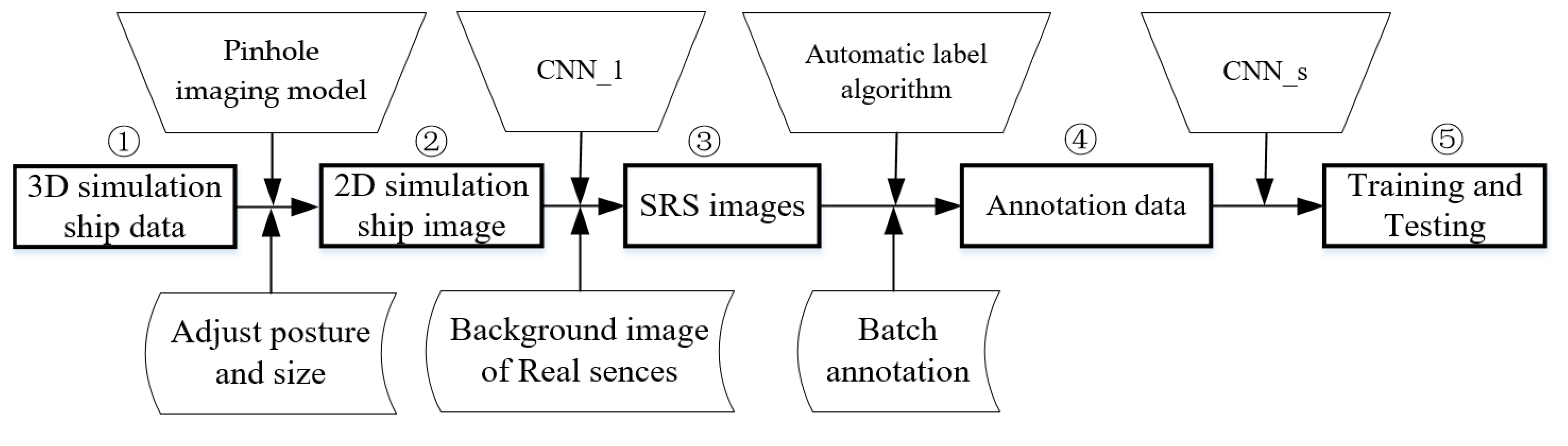
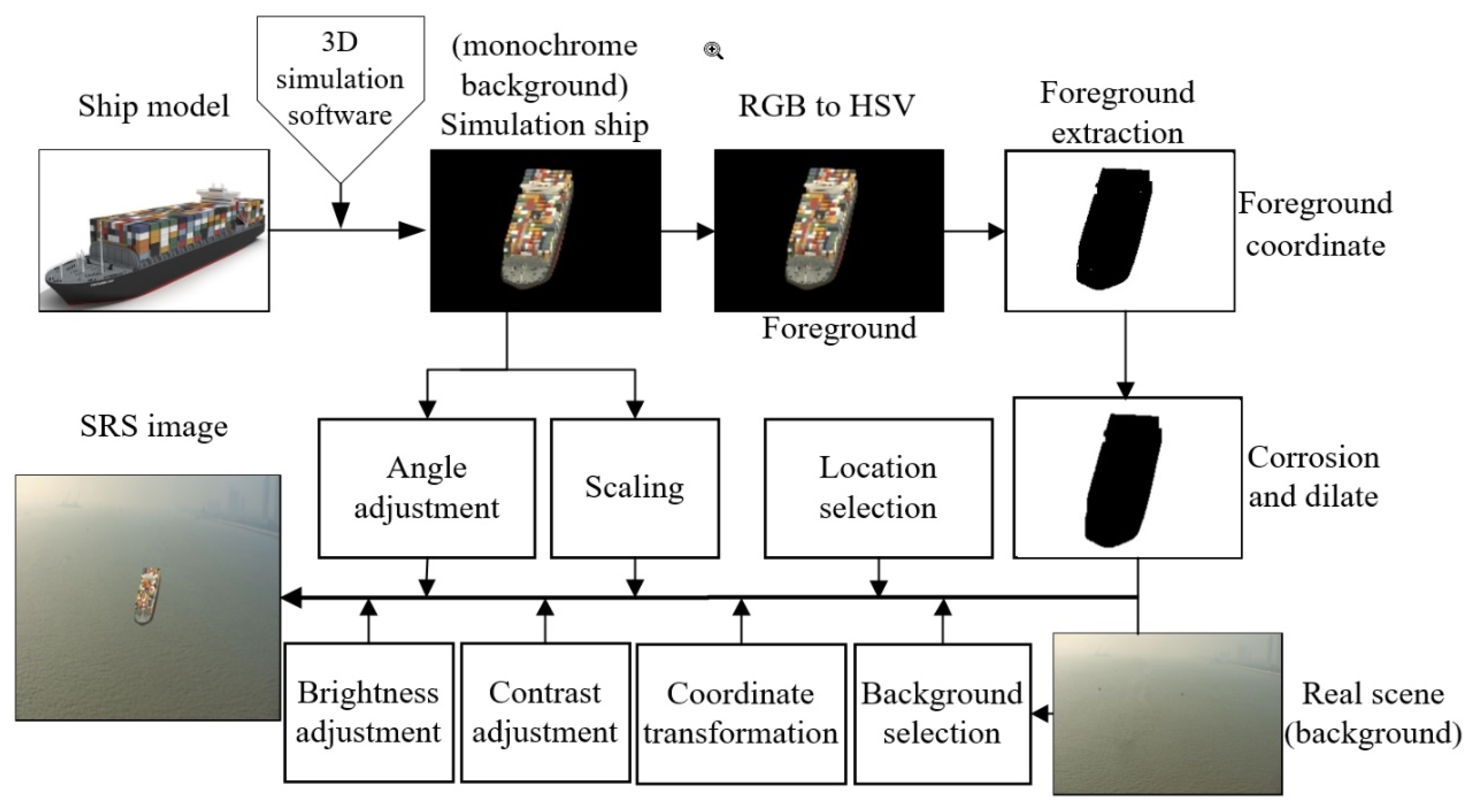
2.1. The Proposed Method of SRS Images Generation

This paper used different kinds of real ship images, which are taken from real experiment scenes as samples to design simulated ship models with 3D software. We then obtained many 3D ship data by changing the parameters in the 3D software. After the 3D data were converted into 2D data, the 2D simulation ship data weresuperimposed into the real scene background to form an SRS image, and we annotated the SRS image with the automatic annotation algorithm at the same time. The main workflow is shown in Figure 1.

2.1.1. 2D Ship Image Generation from 3D Ship Model

The essence of the 3D ship model in practical applications is a 3D point cloud. Therefore, we can use the following set of 3D coordinate points to represent the 3D ship model:

$$S=F(\begin{array}{ccc}{X}_i& Y_i& Z_i\end{array})=\left\{{\left[\begin{array}{ccc}{X}_i& Y_i& Z_i\end{array}\right]}^T\right\}(i=1,2,\cdots ,n)$$

(1)

The principle of pinhole imaging, which is used to convert 3D data into a 2D image, is as follows:

$${[\begin{array}{ccc}{u}_i& v_i& 1\end{array}]}^T\cong K[\begin{array}{cc}R& t\end{array}]{[\begin{array}{cccc}{X}_i& Y_i& Z_i& 1\end{array}]}^T$$

(2)

where $[\begin{array}{ccc}{X}_i& Y_i& Z_i\end{array}]$ are the 3D coordinates of any point on a 3D target ship, and $[\begin{array}{cc}{u}_i& v_i\end{array}]$ is the coordinate of the corresponding image point. $K$ is the camera’s internal parameter matrix; it can be expressed by an upper triangular matrix, as follows:

$$K=\left[\begin{array}{ccc}{f}_u& \varsigma & u_0\\ 0& f_v& v_0\\ 0& 0& 1\end{array}\right]$$

(3)

where $f_u$ and $f_v$ represent the focal length of the camera in terms of pixel dimensions in the $u$ and $v$ direction, respectively, and $[u_0,v_0]$ is the principal point in terms of pixel dimensions. The size of the ship in the image is changed by adjusting the focal length of the camera. Besides the internal parameter matrix of the camera, Formula (2) also involves the rotation matrix and translation vector. The rotation matrix represents the camera’s shooting angle, and the translation vector represents the shooting position of the camera. The ship images from different perpectives can be generated by changing the shooting angle, location of the camera, and focal length. Therefore, we obtained abundant target ship images.

Through the imaging Formulas (1)–(3), 3D points cloud in a 3D ship model can be converted into 2D image data. Therefore, the point set $f(u_i,v_i)$ can also be used to represent the ship’s coordinates in the image. The representation of the point set $f(u_i,v_i)$ is as follows:

$$f(\begin{array}{cc}{u}_i& v_i\end{array})=\left\{{[\begin{array}{cc}{u}_i& v_i\end{array}]}^T\right\}(i=1,2,\cdots n)$$

(4)

Next, we need to extract the points belonging to the simulated ship from the 2D image point set, and add these points to the real experimental scene background.

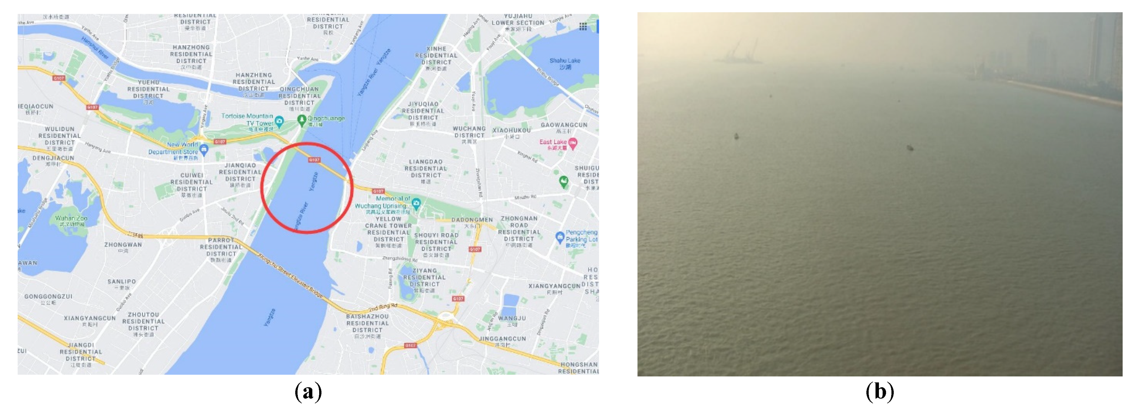
2.1.2. Selection of the Background Images

In this study, the selected experimental location is shown in Figure 2a. Figure 2b is the experimental scene image used as the background image of the SRS images.

As shown in Figure 2, the ship is sailing in a straight inland waterway. In this paper, it is assumed that the ship’s posture is fixed. Therefore, we manually selected the ship posture close to the actual situation before the experiment.

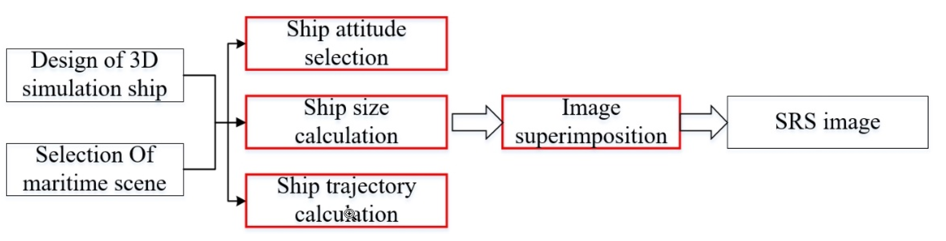
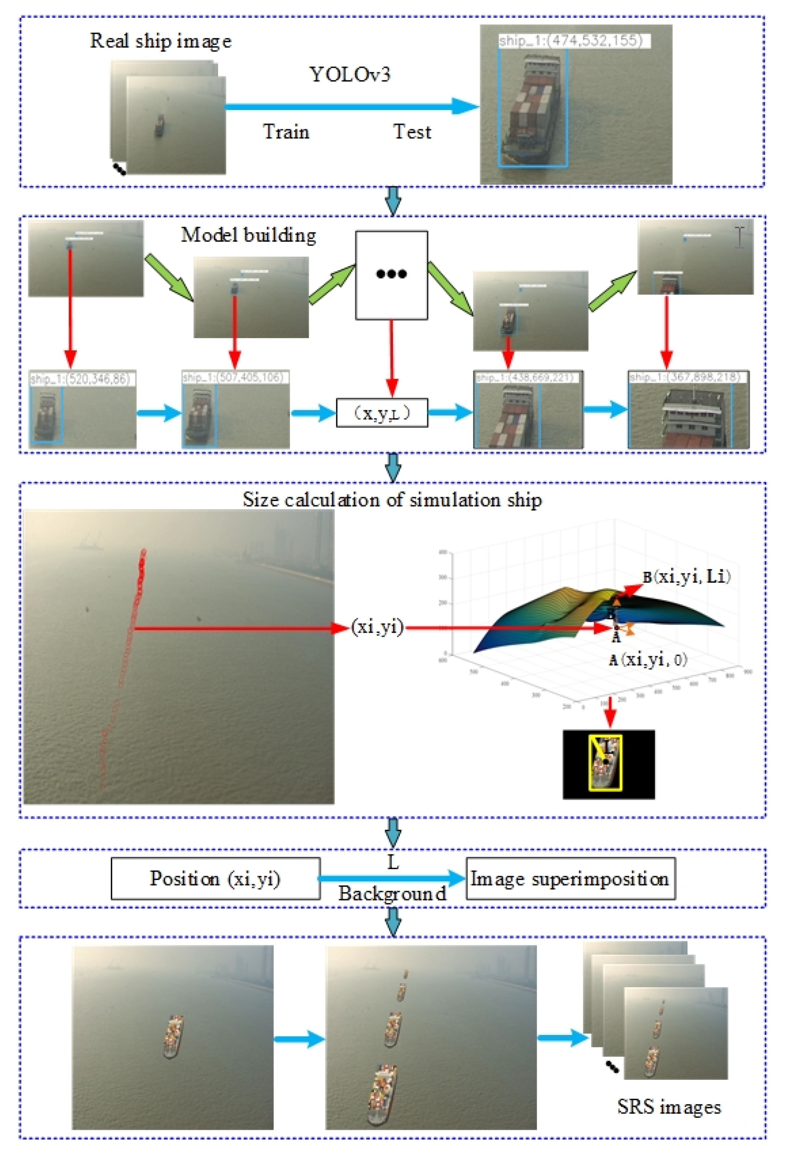
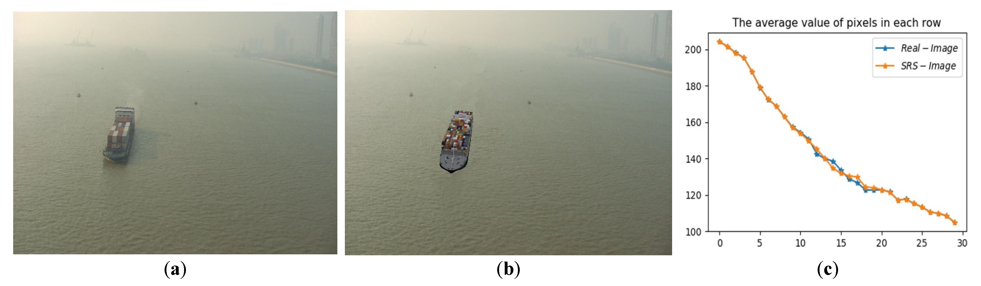
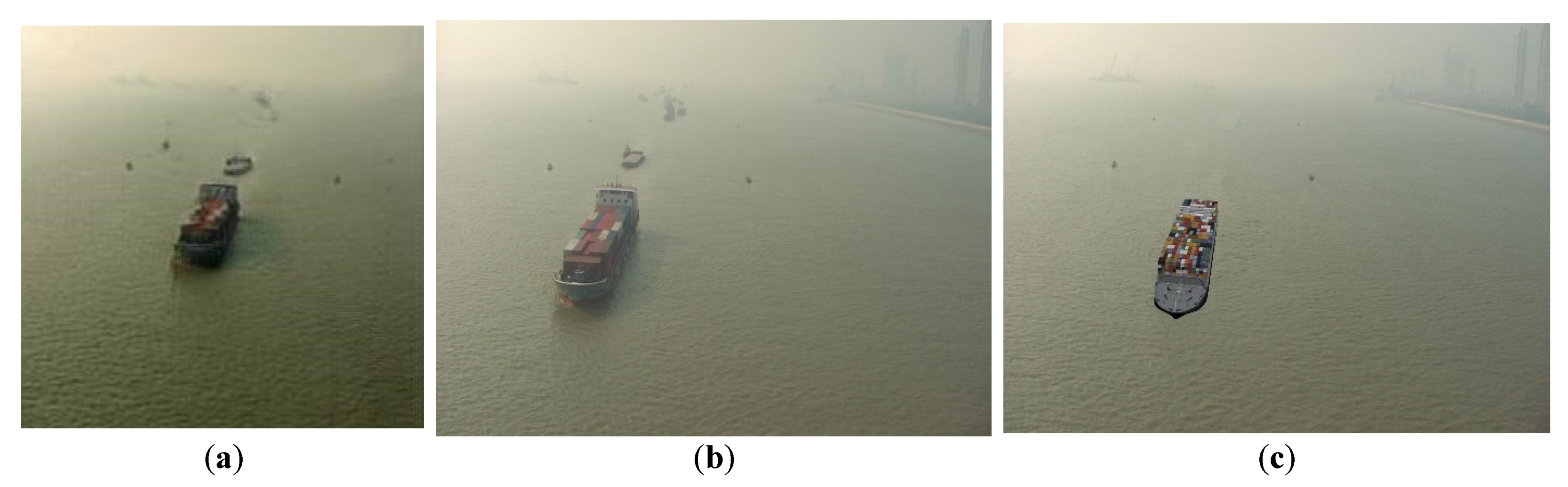
2.1.3. SRS Image Generation

The generation process of the simulation ship mainly includes the steps shown in Figure 3. The red box in Figure 3 is the key to the whole generation process. The next section provides a detailed description of the parts in the red box.

Calculate the Size of the Simulation Ships

Figure 3 briefly illustrates the generation method of the simulated real ship image: the simulated ship is extracted from the simulated ship image and superimposed into the real experimental background scene to form the simulated real ship image. However, there is no clear explanation for the scale, pose, and superimposed position of the simulated ship in the simulated real ship image. The scale calculation method of the simulated ship in the simulated real ship image is as follows:

$$(U_{\mathrm{j}},V_j)={\lambda }_j·(u_j,v_j)$$

(5)

where $(u_j,v_j)$ is the size of the simulated ship, ${\lambda }_j$ is the scale factor, and $(U_j,V_j)$ is the ship image after the scale change.

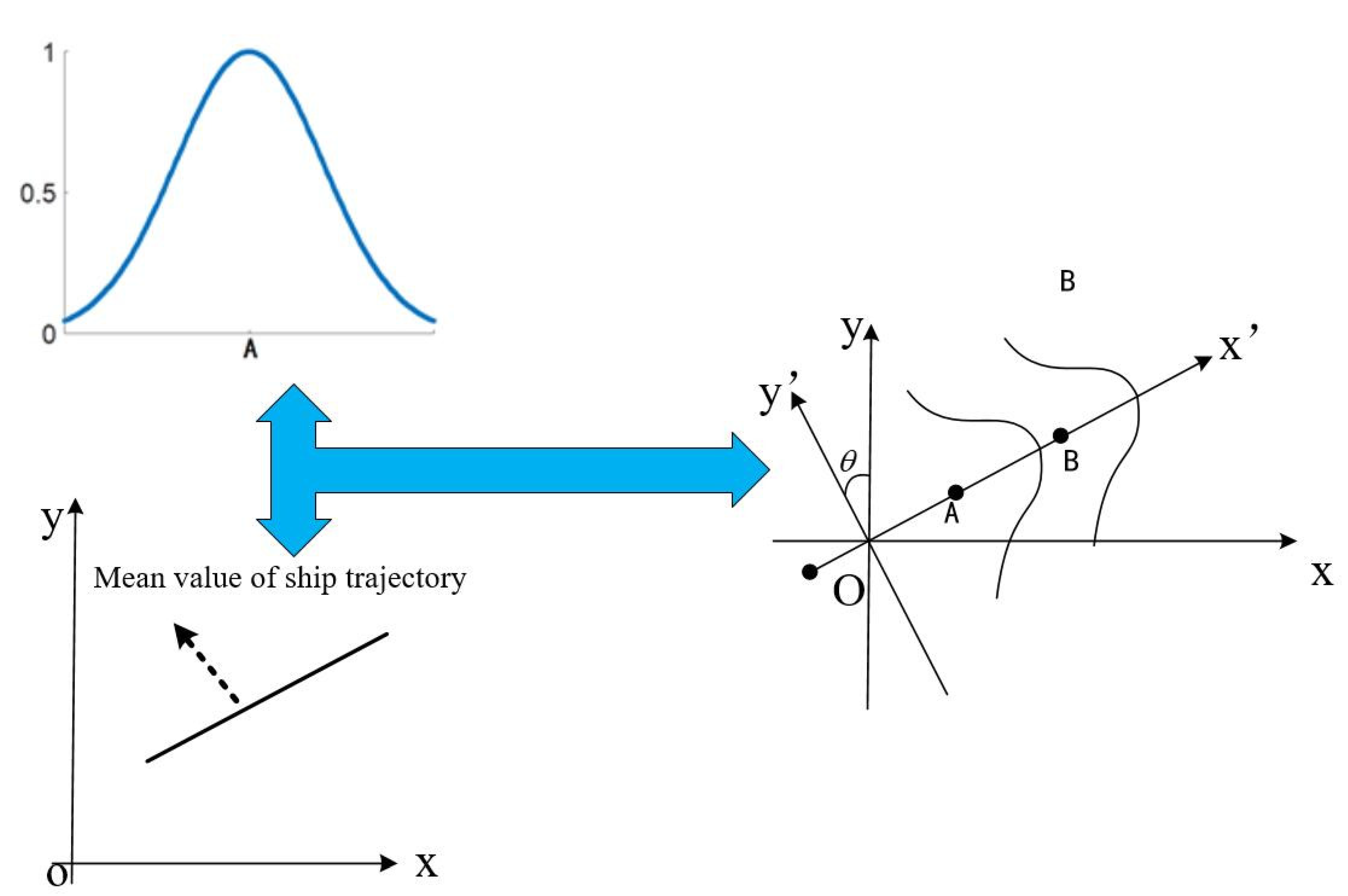
Calculate the Trajectory of Simulation Ships

As shown in Figure 4, suppose the length and height of the bounding box of the simulation ship are $h$ (pixel) and $w$ (pixel), respectively. The distance between the center point of the bounding box and the four corners of the bounding box is $L$. Here, set $L$ as the size of the simulation ship. The size (pixel) of $L$ is:

$$L=\sqrt{{\left(\frac{h}{2}\right)}^2+{\left(\frac{w}{2}\right)}^2}$$

(6)

As shown in Figure 4, the length and height of the bounding box of the simulated ship are $h$ (pixels) and $w$ (pixels), respectively. The distance from the center of the bounding box to the four corners of the bounding box is $L$. The center point of the simulated ship are the coordinates $(x_1,y_1)$ of the simulated ship in the background image. $L$ is the size of the simulated ship (pixels).

Sailing ships need to follow navigation rules, and they must navigate within the area marked by the buoy boats. Both lines connecting the position of the buoy boats refers to the red dashed line in Figure 4. Passing ships must navigate within the area enclosed by the two red dotted lines. We considered the posture of the simulated ship fixed due to the unchanged sailing direction. Next, we analyzed the trajectory of the simulated ship in the background image, as shown in Figure 5.

$$\left[\begin{array}{c}{x}^{\prime }\\ f^{\prime }(x^{\prime })\end{array}\right]=\left[\begin{array}{cc}cos\theta & sin\theta \\ -sin\theta & cos\theta \end{array}\right]\left[\begin{array}{c}x\\ f(x)\end{array}\right]$$

(7)

$$f^{\prime }\left(x^{\prime }\right)=-x·sin\theta +f\left(x\right)·sin\theta +\lambda ·\frac{1}{\sqrt{2\pi }\sigma }exp(-\frac{{((x·cos\theta +f(x)·sin\theta )-\mu )}^2}{2{\sigma }^2})$$

(8)

where $(x,f(x))$ is the coordinate of the simulation ship in the background image, and $(x^{\prime },f(x^{\prime }))$ is the coordinate of the simulation ship after the $\theta$ degree rotation of the coordinate axis. The trajectories of the ships in the maritime scene are distributed around the X-axis. Firstly, we calculated the mean value of the ship’s trajectory, and then the navigation coordinates of the SRS image were obtained by adding Gaussian distribution parameters. The trajectory of the simulation ships in the real scene can be calculated through this method.

Image Superimposition of Target Ship Extracted from the 2D Ship Image and Selected Maritime Scene Background

In the above, the pinhole imaging model was used to transform the 3D ship data into a 2D image, and then we calculated the position and size of the simulation ship and confirmed the posture of the simulation ship. The nest task is to extract the target ship from the 2D ship image with a monochromatic background, and overlay it onto the selected maritime background scene image to form SRS images.

The flow chart of image superimposition is shown in Figure 6. The SRS images point set is as follows:

$$f(x_i,y_i)=(1-a)·f(p_i,t_i)+a·f(u_i,v_i)\begin{array}{ccc}& a\in (0,1)& (i=1,2,\cdots n)\end{array}$$

(9)

where $f(u_i,v_i)$ is the simulation ship image point set, $f(p_i,t_i)$ is the real scene image point set, and $f(x_i,y_i)$ is the SRS images point set.

Generation of SRS Images

Simulation ships in SRS images have three elements: trajectory, size, and posture. The experiments in the experimental scenario are shown in Figure 2; the observation perspective does not change in this scene, and the navigation posture of the ship is assumed to be unchanged or slightly changed. We needed to select the sailing posture before the experiment. The size L of the ship is related to the position of the simulated ship in the background image. In the experiment, we used the YOLO algorithm [12] for modeling, as shown in Figure 7. Coordinates (x1, y1) and L are used to form three-dimensional coordinates (x1, y1, L1) which are the position of the ship in the SRS image. Then, we used the YOLO algorithm to count the data (x1, y1, L1) of 100 ships (cargo ships, passenger ships, sand ships, and small ships.) in the experimental scene, and performed modeling. We determined L by simulating the position of the ship (xi, yi). Finally, the ships’ trajectories were determined based on the voyage data of 100 ships in the experimental scene. The overall flow chart of the SRS image generation method is shown in Figure 7.

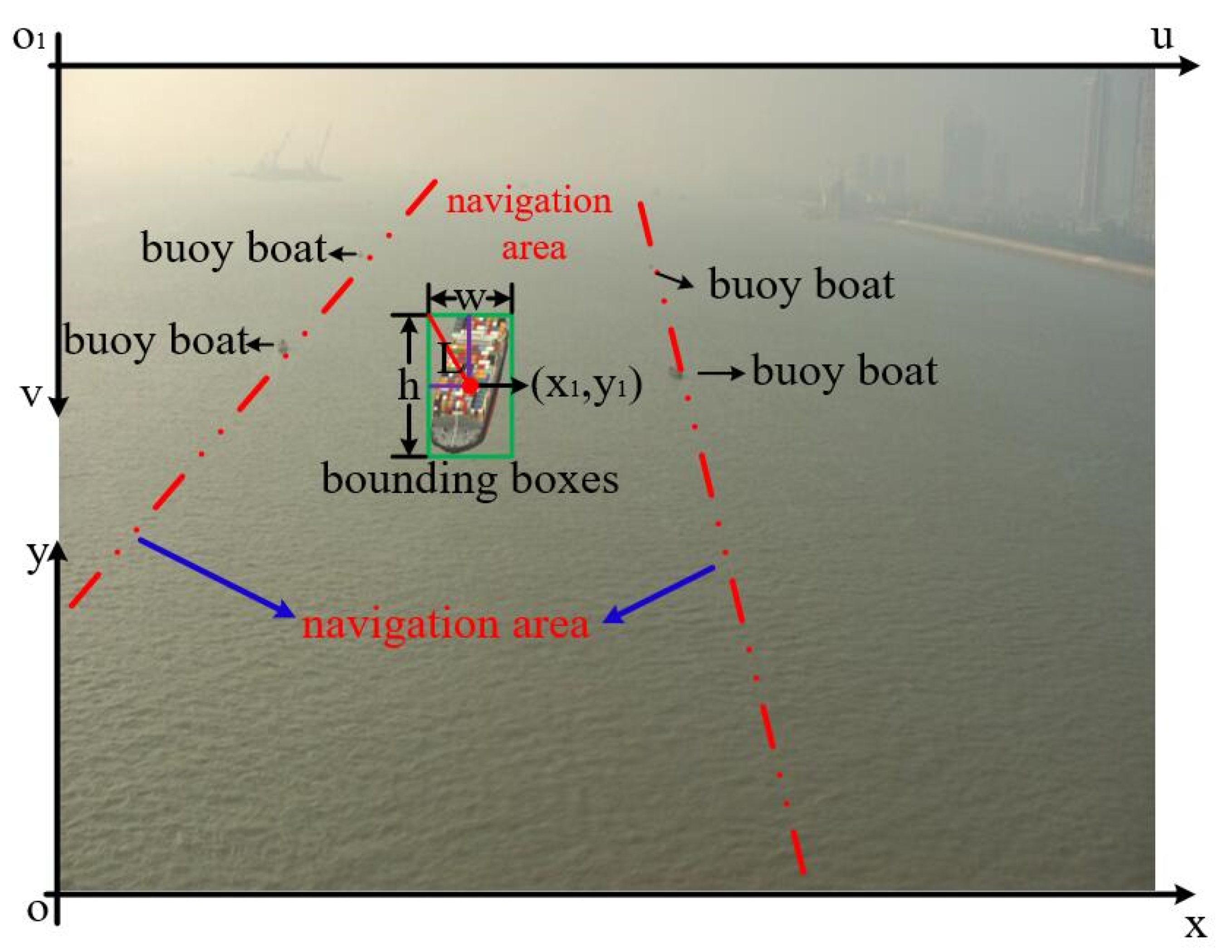
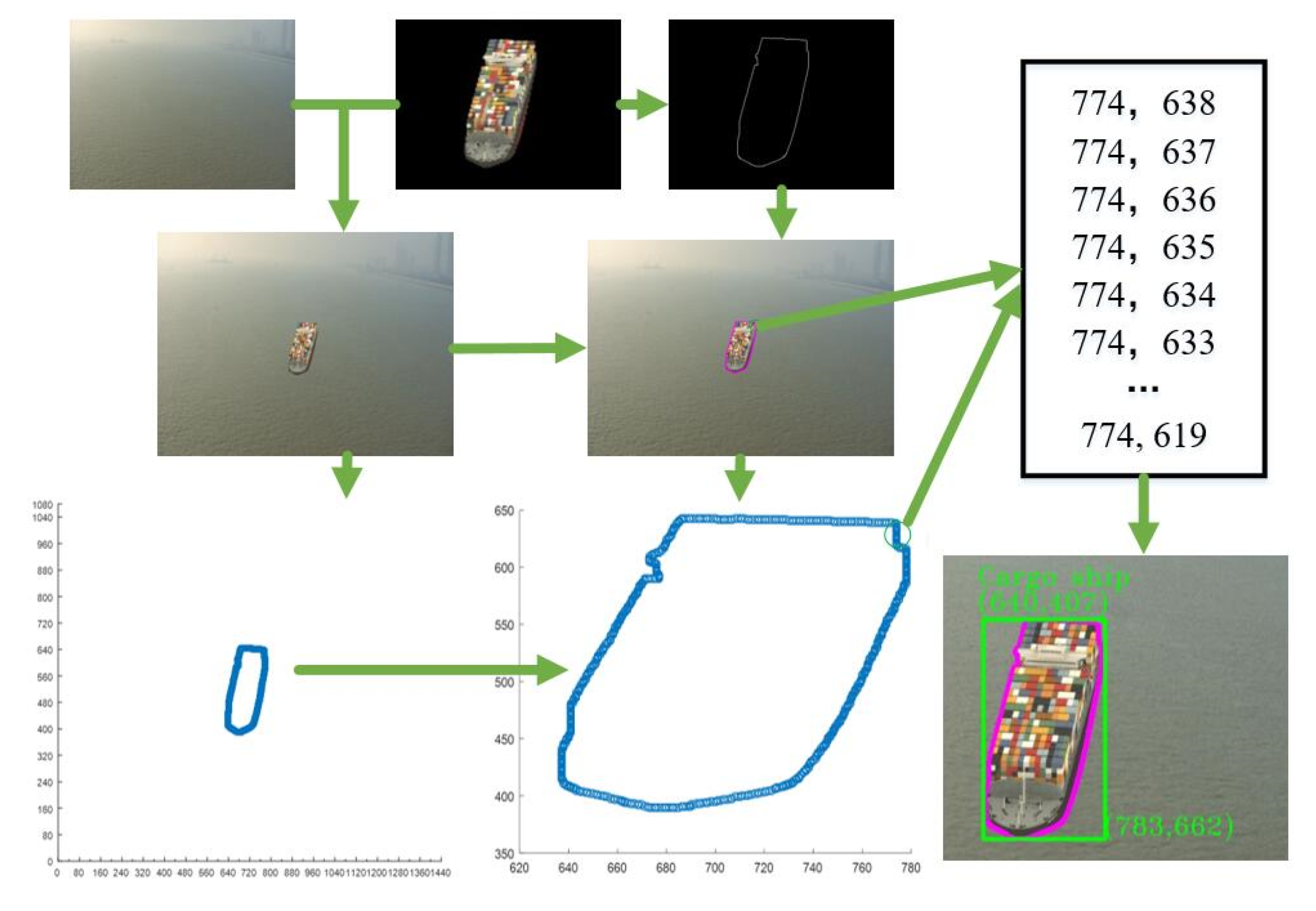
2.2. Automatic Annotation of Target Ship

CNN is a typical supervised learning method, which needs to be trained with annotated data to generate different target detectors. The specific location of the ship target remains unknown in real image data. It usually depends on manual operation for the selection ofthe target contour points to complete the annotation.

It often takes dozens of mouse clicks or more to complete a ship annotation. The annotation is affected by the annotated image’s pixels, which often differ significantly from the actual outline. This paper proposes an automatic annotation method for annotating batch image data. The main flow chart of the proposed annotation method is shown in Figure 8.

First, we extracted the ship contour from the simulation ship image with the monochromatic background. Next, we superimposed the foreground ship image on the background. Thus, the contour of the foreground ship is the contour of the ship in the SRS image. The final task is to represent the contour of the ship in the SRS image in the form of an annotation file.

2.3. Selecting the Typical CNN Algorithm for Training and Testing

To verify the effectiveness of the proposed methods (the SRS image data generation method and the automatic image annotation method), two CNN algorithms, FCN [14], and Mask RCNN [15], were selected to verify the results.

The Mask RCNN algorithm, developed based on Faster RCNN, was proposed by He Kaiming’s team in 2018. This algorithm segments the target in the image. Moreover, the algorithm also derives indicators such as the target object’s position in the image and its reliability. Structurally speaking, Rol Align is introduced to replace Rol Pooling to ensure the accurate semantics segmentation of the target object at the expense of part of the detection time.

The FCN algorithm, proposed by Evan Shelhamer’s team in 2017, classifies images at the pixel level. The size of the input image of the traditional CNN algorithm is fixed during training due to the application of the full connection layer. The FCN algorithm uses a convolutional layer instead of the entire connection layer to regulate the image size during training.

Usually, the object detection algorithm based on deep learning can be divided into boundary box recognition and semantic segmentation recognition according to object recognition manner. Both algorithms use the bounding box and image segmentation to separate the object from the image. The second method obtains more abundant pixel information of the object. Therefore, this study selected Mask RCNN and FCN based on semantic segmentation to verify the results.

3. Results

3.1. Experiment Platform and Parameter Settings

The experimental configuration was as follows: CPU: Intel Core i7-8700K; Memory: 16G, GPU: NVidia GeForce GTX 1660; Operating system: Ubuntu 16.04.

We completed the experiment with the V2T_ShipData dataset of V2T Laboratory of Wuhan University of Technology. We selected 100 items of sailing data of real ships for the experiments. Among them, there were 25 cargo ships, passenger ships, sand ships, and small ships. Five pictures of one ship were selected for experimental testing. Therefore, a total of 500 ship sample images were used for this experiment’s training and detection task.

3.2. Generation and Automatic Annotating of SRS Images Data

In this experiment, four typical ships sailing in the Yangtze River were selected for experiments and modeling. The results of the modeling are shown in Figure 9.

As shown in Figure 9, the dimension L and coordinates (x and y) of 25 sailing ships in the actual scene were detected by the YOLO algorithm to construct a 3D curved surface. The coordinates (trajectories) of the simulation ship can be calculated by Formula (9). The dimension L of the ship can be calculated by the curved surface and the coordinates of the ship. The posture of the simulation ship was selected manually. Therefore, all three elements of SRS images were obtained. The SRS images generated by the proposed method are shown in Figure 10a,b.

In this experiment, we used two annotation methods to label the four kinds of ships, as shown in Figure 10c. The annotation methods, bounding box method (green box in Figure 10c), and outline method (red line in Figure 10c) were used to label SRS images. Simultaneously, the names of the targets were displayed on the top left of the labeled targets.

3.3. Training and Detection with Mask RCNN and FCN

The Mask RCNN and FCN algorithms were selected to test the generated dataset in this paper.

In this study, 500 images were selected for the experiment from 10,000 SRS images. There were 125 images of cargo ships, passenger ships, sand ships, and small ships. These 500 ship images were used as training samples of the two algorithms (Mask RCNN and FCN). Then, the 500 real ship images mentioned above were used as the sample data for detection.

The detection samples of both algorithms are shown in Figure 11.

4. Discussion

4.1. Comparative Experiment 1: Comparing Our Annotation Method with the Existing Annotation Method

In this paper, the automatic labeling algorithm and manual labeling method proposed were used to label the cargo ship, which was taken as an example. The labeling results are shown in Figure 12.

The annotation results of the manual annotation are shown in Figure 12a. The annotation results of the automatic annotation algorithm proposed (the blue line in Figure 12b) accurately labeled the object in the image. The comparison results of both annotation methods are shown in Figure 12c; the manual annotation method (the blue line in Figure 12a) easily labeled the non-target pixels as target pixels but the proposed annotation method did not have this situation. The automatic annotation method proposed was able to label the contour and the boundary box of the targetat the same time. The manual annotation method can only label one by one, but the proposed annotation method can carry out batch annotation.

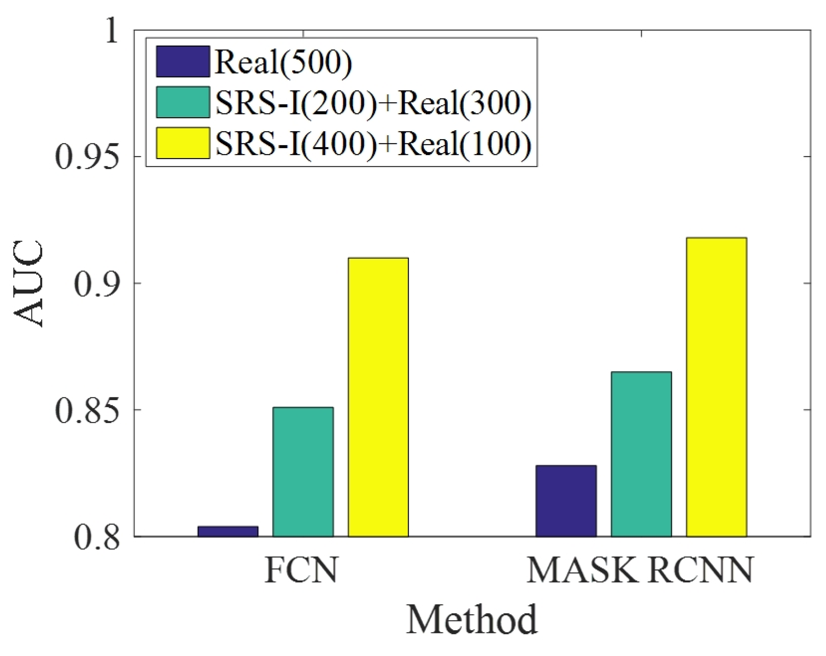
4.2. Comparative Experiment 2: Comparing the SRS Images with the Real Scene Ship Image

The similarity between the SRS images and the real ship image is the key of the study. We selected a real ship image and an SRS image with the same background to detect the similarity between both. Figure 13a is a real ship image, and Figure 13b is an SRS image. We took pixels as the research object for modeling. The average value of each row of pixels in the two images was calculated (Figure 13c). The results show that the designed SRS images have a high similarity with the real ship image.

In order to further verify the effectiveness of the SRS image, we took two kinds of data, which are real ship images and SRS images, as training data and took real images as testing data to carry out experiments. The experiment included three steps: first, all the training data were real images. Then, we took 300 real images and 200 simulation images as training data. Finally, we took 100 real images and 400 simulation images as training data. Taking Mask RCNN and FCN as training and testing methods, the experimental design and results are shown in

Table 1. Test results of similar data sets.

Training and Testing Method	Type of Data for Training (Number)	Type of Data for Testing (Number)	Accuracy (%)	TPR (%)	FPR (%)
FCN	Real(500)	Real(500)	84.2	86.4	19.1
	Real(300) + SRS-I(200)		88.5	90.8	11.8
	Real(100) + SRS-I(400)		91.3	92.8	9.2
Mask RCNN	Real(500)	Real(500)	86.3	88.5	17.6
	Real(300) + SRS-I(200)		90.6	93.2	10.6
	Real(100) + SRS-I(400)		92.9	94.5	7.6

.

Table 1 shows the results of different detection methods combined with various image dataset. According to the results of FCN, “SRS-I(400) + Real(100)” achieves the highest accuracy rate (91.3%), followed by “SRS-I(200) + Real(300)” (88.5%), “Real(500)” (84.2%), “SRS-I(400) + Real(100)” (TPR: 92.8% and FPR: 9.2%) outperformed the compared methods, as confirmed by the results of the true positive rate (TPR) and false positive rate (FPR). The FPR of the proposed method was the lowest among the compared methods.Moreover, “SRS-I(400) + Real(100)” demonstrated the highest AUC (0.910). Therefore, the dataset generated by the proposed method was more effective than the real dataset selected by us (Figure 14). The detection results of Mask RCNN, “SRS-I(400) + Real(100)” achieved the highest accuracy rate (92.9%), followed by “SRS-I(200) + Real(300)” (90.6%), “Real(500)” (86.3%).

“SRS-I(400) + Real(100)” (TPR: 94.5% and FPR: 7.6%) outperformed the compared methods according to the true positive rate (TPR) and false positive rate (FPR). The FPR of the proposed method was the lowest among the compared methods. Therefore, the dataset generated by the proposed method was more effective than the other compared datasets, as confirmed by the highest AUC (0.918) (see Figure 14).

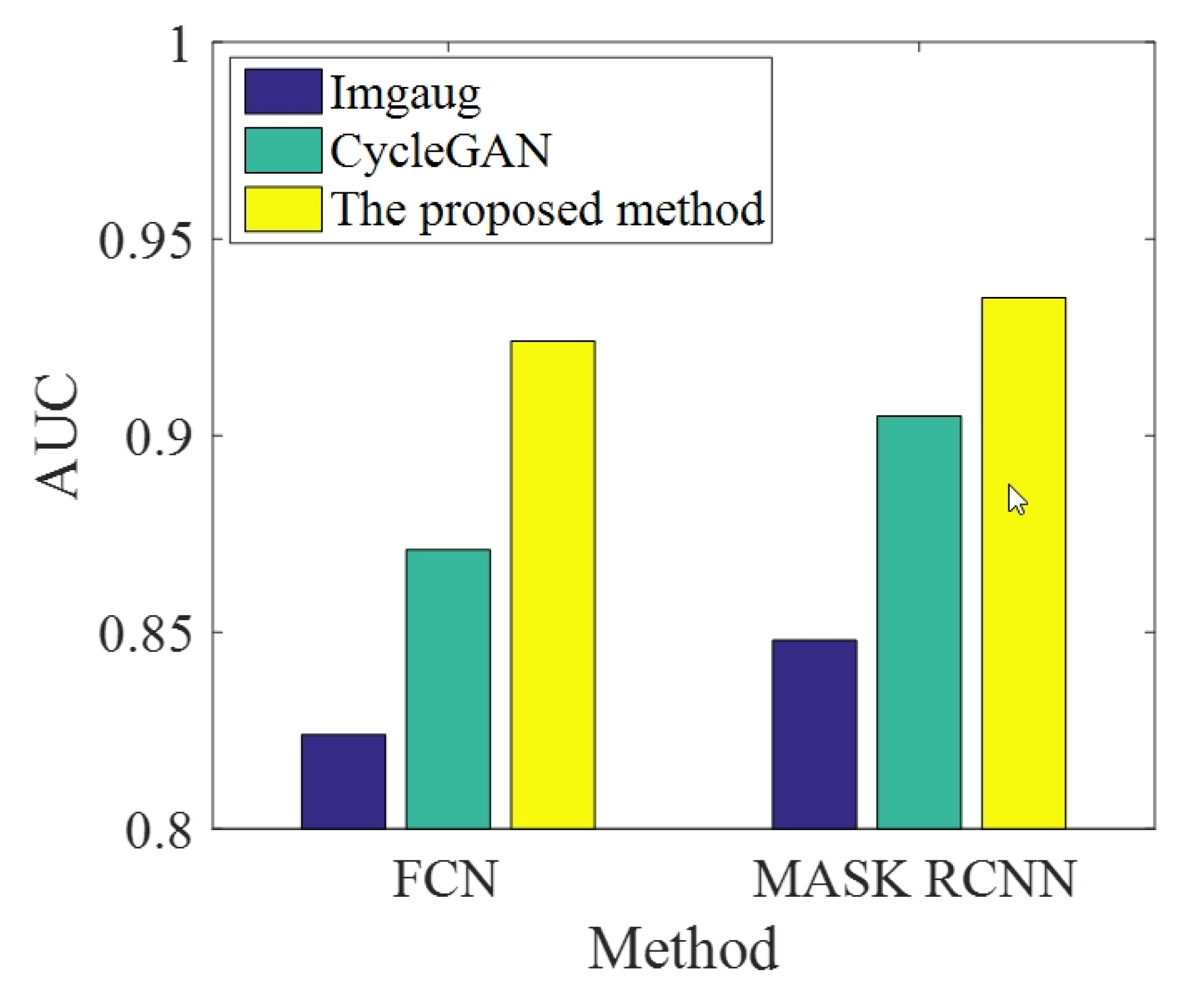
4.3. Comparative Experiment 3: Comparison with the Existing Data Augmentation Methods

At present, the common data augmentation methods, such as Imgaug [41], have the core idea of pixel transformation of 2D images. The transformation methods, such as rotation, translation, flipping, scaling, and clipping, increased the number of samples.

The target detection algorithm based on deep learning needs many image data for training, extracting sufficient target features from the image data, and generating the target detector. The abundant target features extracted from the training data guaranteed the detection accuracy. Traditional data enhancement methods increase the amount of data by changing the scale, posture and color of the existing 2D image but the actual enhancement of image features is limited.

GAN [29], an unsupervised deep learning algorithm, is a classic data augmentation method. GAN aims to fit the distribution of the sample set to obtain highly qualified samples based on zero-sum game theory. The GAN algorithm generated simulation images highly similar to the real images. The simulation ship images generated by CycleGAN were used for deep learning training and testing in this paper. The simulation ship generated by the CycleGAN algorithm [30] after 500 epochs is shown in Figure 15a. The SRS image shown in Figure 15c has a much higher definition and clearer contour than the image shown in Figure 15a.

Table 2. Test results of similar data sets.

Training and Testing Method	Type of Data for Training (Number)	Type of Data for Testing (Number)	Accuracy (%)	TPR (%)	FPR (%)
FCN	Imgaug [41]	Real(500)	85.7	88.9	17.1
	CycleGAN [30]		90.9	91.5	11.2
	Our method		93.2	94.4	7.1
Mask RCNN	Imgaug [41]	Real(500)	87.3	89.5	14.6
	CycleGAN [30]		91.7	93.1	10.5
	Our method		94.6	95.7	5.6

shows the results of different detection methods combined with various image datasets. According to the results of FCN, the proposed method achieved the highest accuracy rate (93.2%), followed by CycleGAN (90.9%), Imgaug (85.7%). The proposed method (TPR: 94.4% and FPR: 7.1%) outperformed the compared methods, as confirmed by the results of the true positive rate (TPR) and false positive rate (FPR). The FPR of the proposed method was the lowest among the compared methods. Moreover, the proposed method demonstrated the highest AUC (0.924). Therefore, the dataset generated by the proposed method was more effective than other compared datasets (Figure 16). The detection results of Mask RCNN, the proposed method achieved the highest accuracy rate (94.6%), followed by CycleGAN (91.7%) and Imgaug (87.3%).

The proposed method (TPR: 95.7% and FPR: 5.6%) outperformed the compared methods according to the true positive rate (TPR) and false positive rate (FPR). The FPR of the proposed method was the lowest among the compared methods. Therefore, the dataset generated by the proposed method was more effective than the other compared datasets, as confirmed by the highest AUC (0.935) (see Figure 16).

5. Conclusions

This study proposes a novel ship image generation method and a novel ship image annotation method. The proposed method was developed based on a 3D simulated ship and CNN algorithms. Firstly, a large number of simulation ships were generated by 3D simulation software. The experimental image scene used as the background image was selected. Secondly, the proposed generation method of simulated ship images includes three key parts: (1) the posture of the simulation ship; (2) the trajectory of the ship; (3) the size of the ship. The postures of the simulation ships areselected manually according to the actual navigation posture of the ships; the trajectory and the size of the simulation ship can be computed with the model proposed in this paper. There was a high degree of similarity between the SRS image and the ship image of the real scene. The experimental results show that the SRS images achieved a higher detection accuracy than the same number of the ship images. The automatic annotation methods proposed can be used as a bounding box annotation and contour annotation. The ship image data set and automatic annotation program of this study will be published subsequently.

There are still some problems to be solved in this study. First, we manually selected the posture of the 3D simulation ship according to the posture of the ship in the real scene. In a follow-upwork, the proposed method will automatically identify the ship’s posture in the real scene, on this basis, it will automatically set the 3D simulation ship posture. Second, there were about 20 kinds of ships in the 3D simulation ship dataset; thus, the number of ship types and the similarity between SRS images and real ship images need to be increased. Third, we calculated the position and the size of the simulation ship in Euclidean space. In the follow-up work, time-domain and frequency-domain characteristics will be used to calculate the position of the target ship in SRS images.

References

1. Ferdinand, P. Westward ho—The China dream and ‘one belt, one road’: Chinese foreign policy under Xi Jinping. Int. Aff. 2016, 92, 941–957. [Google Scholar] [CrossRef] [Green Version]
2. Blanchard, J.-M.F.; Flint, C. The Geopolitics of China’s Maritime Silk Road Initiative. Geopolitics 2017, 22, 223–245. [Google Scholar] [CrossRef]
3. Chen, Z.; Chen, D.; Zhang, Y.; Cheng, X.; Zhang, M.; Wu, C. Deep learning for autonomous ship-oriented small ship detection. Saf. Sci. 2020, 130, 104812. [Google Scholar] [CrossRef]
4. Girshick, R.; Donahue, J.; Darrell, T.; Malik, J. Rich Feature Hierarchies for Accurate Object Detection and Semantic Segmentation. In Proceedings of the 2014 IEEE Conference on Computer Vision and Pattern Recognition, Columbus, OH, USA, 20–23 June 2014; pp. 580–587. [Google Scholar]
5. He, K.M.; Zhang, X.Y.; Ren, S.Q.; Sun, J. Spatial Pyramid Pooling in Deep Convolutional Networks for Visual Recognition. IEEE Trans. Pattern Anal. Mach. Intell. 2014, 37, 1904–1916. [Google Scholar] [CrossRef] [PubMed] [Green Version]
6. Girshick, R.B. Fast R-CNN. In Proceedings of the 2015 IEEE International Conference on Computer Vision (ICCV), Santiago, Chile, 13–16 December 2015; pp. 1440–1448. [Google Scholar]
7. Dai, J.; Li, Y.; He, K. R-fcn: Object detection via region-based fully convolutional networks. arXiv 2016, arXiv:1605.06409. Available online: https://arxiv.org/pdf/1605.06409.pdf (accessed on 25 March 2021).
8. Ren, S.Q.; He, K.M.; Girshick, R. Faster r-cnn: Towards real-time object detection with region proposal networks. arXiv 2015, arXiv:1506.01497. Available online: https://arxiv.org/pdf/1506.01497.pdf (accessed on 25 March 2021). [CrossRef] [PubMed] [Green Version]
9. Redmon, J.; Divvala, S.; Girshick, R.; Farhadi, A. You Only Look Once: Unified, Real-Time Object Detection. In Proceedings of the 2016 IEEE Conference on Computer Vision and Pattern Recognition (CVPR), Las Vegas, NV, USA, 27–30 June 2016; pp. 779–788. [Google Scholar]
10. Redmon, J.; Farhadi, A. YOLO9000: Better, Faster, Stronger. In Proceedings of the 2017 IEEE Conference on Computer Vision and Pattern Recognition (CVPR), Honolulu, HI, USA, 21–26 July 2017; pp. 6517–6525. [Google Scholar]
11. Redmon, J.; Farhadi, A. Yolov3: An incremental improvement. arXiv 2018, arXiv:1804.02767. [Google Scholar]
12. Bochkovskiy, A.; Wang, C.Y.; Liao, H.Y.M. Yolov4: Optimal speed and accuracy of object detection. arXiv 2020, arXiv:2004.10934. [Google Scholar]
13. Liu, W.; Anguelov, D.; Erhan, D. Ssd: Single shot multibox detector. In Proceedings of the 14th European Conference on Computer Vision, Amsterdam, The Netherlands, 8–16 October 2016; pp. 21–37. [Google Scholar]
14. Long, J.; Shelhamer, E.; Darrell, T. Fully convolutional networks for semantic segmentation. In Proceedings of the 2015 IEEE Conference on Computer Vision and Pattern Recognition (CVPR), Boston, MA, USA, 8–10 June 2015; pp. 3431–3440. [Google Scholar]
15. He, K.M.; Gkioxari, G.; Dollár, P.; Girshick, R. Mask r-cnn. In Proceedings of the 2017 IEEE International Conference on Computer Vision, Venice, Italy, 22–29 October 2017; pp. 2961–2969. [Google Scholar]
16. Ye, F.; Yang, J. A Deep Neural Network Model for Speaker Identification. Appl. Sci. 2021, 11, 3603. [Google Scholar] [CrossRef]
17. Fleet, D.; Pajdla, T.; Schiele, B.; Tuytelaars, T. Microsoft coco: Common objects in context. In Proceedings of the 13th European Conference on Computer Vision, Zurich, Switzerland, 6–12 September 2014; pp. 740–755. [Google Scholar]
18. Kuznetsova, A.; Rom, H.; Alldrin, N. The open images dataset v4: Unified image classification, object detection, and visual relationship detection at scale. arXiv 2018, arXiv:1811.00982. Available online: https://doi.org/10.1007/s11263-020-01316-z (accessed on 25 March 2021). [CrossRef] [Green Version]
19. Krizhevsky, A.; Sutskever, I.; Hinton, G.E. ImageNet classification with deep convolutional neural networks. Commun. ACM 2017, 60, 84–90. [Google Scholar] [CrossRef]
20. Deng, J.; Dong, W.; Socher, R. Imagenet: A large-scale hierarchical image database. In Proceedings of the 22th IEEE Conference on Computer Vision and Pattern Recognition, Miami Beach, FL, USA, 20–25 June 2009; pp. 248–255. [Google Scholar]
21. Everingham, M.; Van Gool, L.; Williams, C.K.I. The pascal visual object classes (voc) challenge. Int. J. Comput. Vis. 2010, 88, 303–338. [Google Scholar] [CrossRef] [Green Version]
22. Prasad, D.K.; Prasath, C.K.; Rajan, D. Challenges in video based object detection in maritime scenario using computer vision. arXiv 2016, arXiv:1608.01079. [Google Scholar]
23. Cubuk, E.D.; Zoph, B.; Mane, D. Autoaugment: Learning augmentation policies from data. arXiv 2018, arXiv:1805.09501. [Google Scholar]
24. Cubuk, E.D.; Zoph, B.; Shlens, J. Randaugment: Practical automated data augmentation with a reduced search space. In Proceedings of the 2020 IEEE/CVF Conference on Computer Vision and Pattern Recognition Workshops, Seattle, WA, USA, 14–19 June 2020; pp. 702–703. [Google Scholar]
25. Buslaev, A.; Iglovikov, V.I.; Khvedchenya, E. Albumentations: Fast and flexible image augmentations. Information 2020, 11, 125. [Google Scholar] [CrossRef] [Green Version]
26. Chawla, N.V.; Bowyer, K.W.; Hall, L.O. SMOTE: Synthetic minority over-sampling technique. J. Artif. Intell. Res. 2002, 16, 321–357. [Google Scholar] [CrossRef]
27. Goodfellow, I.J.; Pouget-Abadie, J.; Mirza, M. Generative adversarial networks. arXiv 2014, arXiv:1406.2661. [Google Scholar] [CrossRef]
28. Radford, A.; Metz, L.; Chintala, S. Unsupervised representation learning with deep convolutional generative adversarial networks. arXiv 2015, arXiv:1511.06434. [Google Scholar]
29. Mirza, M.; Osindero, S. Conditional generative adversarial nets. arXiv 2014, arXiv:1411.1784. [Google Scholar]
30. Zhu, J.Y.; Park, T.; Isola, P. Unpaired image-to-image translation using cycle-consistent adversarial networks. In Proceedings of the 2017 IEEE International Conference on Computer Vision, Venice, Italy, 22–29 October 2017; pp. 2223–2232. [Google Scholar]
31. Liu, M.Y.; Tuzel, O. Coupled generative adversarial networks. arXiv 2016, arXiv:1606.07536. [Google Scholar]
32. Ledig, C.; Theis, L.; Huszár, F. Photo-realistic single image super-resolution using a generative adversarial network. In Proceedings of the 2017 IEEE Conference on Computer Vision and Pattern Recognition, Honolulu, HI, USA, 21–26 July 2017; pp. 4681–4690. [Google Scholar]
33. Karras, T.; Aila, T.; Laine, S. Progressive growing of gans for improved quality, stability, and variation. arXiv 2017, arXiv:1710.10196. [Google Scholar]
34. Arjovsky, M.; Chintala, S.; Bottou, L.E.O. Wasserstein gan. arXiv 2017, arXiv:1701.07875. [Google Scholar]
35. Zhang, H.; Goodfellow, I.; Metaxas, D. Self-attention generative adversarial networks. In Proceedings of the 2019 International Conference on Machine Learning(PMLR), Ghent, Belgium, 3–6 July 2019; pp. 7354–7363. [Google Scholar]
36. Brock, A.; Donahue, J.; Simonyan, K. Large scale GAN training for high fidelity natural image synthesis. arXiv 2018, arXiv:1809.11096. [Google Scholar]
37. Karras, T.; Laine, S.; Aila, T. A style-based generator architecture for generative adversarial networks. In Proceedings of the 2019 IEEE/CVF Conference on Computer Vision and Pattern Recognition, Los Angeles, CA, USA, 16–19 June 2019; pp. 4401–4410. [Google Scholar]
38. Dewi, C.; Chen, R.C.; Liu, Y.T. Various Generative Adversarial Networks Model for Synthetic Prohibitory Sign Image Gen-eration. Appl. Sci. 2021, 11, 2913. [Google Scholar] [CrossRef]
39. Alruwaili, M.; Siddiqi, M.H.; Javed, M.A. A robust clustering algorithm using spatial fuzzy C-means for brain MR images. Egypt. Inform. J. 2020, 21, 51–66. [Google Scholar] [CrossRef]
40. Versaci, M.; Morabito, F.C. Image edge detection: A new approach based on fuzzy entropy and fuzzy divergence. Int. J. Fuzzy Syst. 2021, 23, 1–19. [Google Scholar] [CrossRef]
41. Jung, A. Imgaug: Image augmentation for machine learning experiments. Accessed 2017, 3, 977–997. [Google Scholar]
Figure 1. The main workflow of this paper. ① is made by the 3D simulation software, and ① is designed according to the appearance of the real ship in the real experiment scene. After adjusting the posture and the size of the 3D simulation ship data with the 3D simulation software, ① is projected onto the 2D plane through a pinhole imaging model, and ② is derived. Then, we superimpose the foreground target (2D ship), which is extracted from ② to the real scene background, so we obtain ③, and we can also obtain ④ by the proposed method. The final task ⑤ is to train and test the SRS image with different CNN algorithms.
Applsci 11 05931 g001
Figure 2. Selection of experimental scene: (a) experimental location, (b) experimental scene image.
Applsci 11 05931 g002
Figure 3. Key steps of SRS images generation.
Applsci 11 05931 g003
Figure 4. Modeling of simulation ship in background scene.
Applsci 11 05931 g004
Figure 5. Trajectory of the generation of SRS images. On the basis of mean value of ship trajectory, Gaussian distribution parameters are added to obtain the navigation trajectory of the simulation ship of the SRS images.
Applsci 11 05931 g005
Figure 6. Flow chart of image superimposition.
Applsci 11 05931 g006
Figure 7. Flow chart of SRS images generation method.
Applsci 11 05931 g007
Figure 8. The automatic annotation method proposed in this paper.
Applsci 11 05931 g008
Figure 9. The size-position model of the four typical ship images: (a) cargo ship; (b) passenger ship; (c) sand ship; (d) small ship.
Applsci 11 05931 g009
Figure 10. Four typical SRS images generated by the proposed method: (a) SRS images with a single object; (b) SRS images with multiple objects; (c) annotation samples.
Applsci 11 05931 g010
Figure 11. Samples of ship detection with Mask RCNN and FCN: (a) detection samples of Mask RCNN; (b) detection samples of FCN.
Applsci 11 05931 g011
Figure 12. Manual annotation and the proposed annotation method: (a) manual annotation method; (b) the proposed annotation method; (c) the results of the annotation.
Applsci 11 05931 g012
Figure 13. Difference between the SRS image and the real ship image: (a) the real ship image; (b) SRS images; (c) contrast curve.
Applsci 11 05931 g013
Figure 14. AUC of the selected methods (algorithm index corresponds to the No. shown in Table 1).
Applsci 11 05931 g014
Figure 15. The simulation ship image generated by different methods: (a) the simulation ship image generated by CycleGAN; (b) the real ship image; (c) the SRS image.
Applsci 11 05931 g015
Figure 16. AUC of the selected methods (algorithm index corresponds to the no. shown in Table 2).
Applsci 11 05931 g016