Diagnosis and Monitoring of Volatile Fatty Acids Production from Raw Cheese Whey by Multiscale Time-Series Analysis

Abstract

Anaerobic treatment is a viable alternative for the treatment of agro-industrial waste. Anaerobic digestion reduces organic load and produces volatile fatty acids (VFA), which are precursors of value-added products such as methane-rich biogas, biohydrogen, and biopolymers. Nowadays, there are no low-cost diagnosis and monitoring systems that analyze the dynamic behavior of key variables in real time, representing a significant limitation for its practical implementation. In this work, the feasibility of using the multiscale analysis to diagnose and monitor the key variables in VFA production by anaerobic treatment of raw cheese whey is presented. First, experiments were carried out to evaluate the performance of the proposed methodology under different operating conditions. Then, experimental pH time series were analyzed using rescaled range (R/S) techniques. Time-series analysis shows that the anaerobic VFA production exhibits a multiscale behavior, identifying three characteristic regions (i.e., three values of Hurst exponent). In addition, the dynamic Hurst exponents show satisfactory correlations with the chemical oxygen demand (COD) consumption and VFA production. The multiscale analysis of pH time series is easy to implement and inexpensive. Hence, it could be used as a diagnosis and indirect monitoring system of key variables in the anaerobic treatment of raw cheese whey.

1. Introduction

Cheese whey is a waste generated in cheese production, which is characterized by its high organic load [1]. Different biological and physicochemical treatments have been proposed to recover compounds with added value, such as proteins and lactose. However, a significant number of small and medium industries do not have the necessary economic resources to implement technologies for the treatment of whey, which leads to the inadequate disposal of the waste, causing serious problems of environmental pollution [2]. Anaerobic treatment is an alternative for the valorization of this effluent. The anaerobic digestion of cheese whey reduces the organic load with simultaneous recovery of value-added by-products such as VFA, methane-rich biogas, biohydrogen, and biopolymers [3,4].

Anaerobic digestion (AD) is a complex and intrinsically unstable process. Indeed, the anaerobic treatment is formed by consecutive stages conducted by a specific group of microorganisms with different metabolic characteristics which are not fully understood. Moreover, variations of the input variables (hydraulic flow rate, influent organic load) and the effects of inhibitory agents may easily lead to the wash-out condition [5].

Thus, proper diagnosis and control of AD are of utmost relevance to avoid serious breakdowns and guarantee operational stability [6,7]. To this end, it is necessary to monitor the variables that provide information on the performance of each stage. The key variables of each stage can be defined by their relationship with the performance of the associated microbial consortium. Indeed, carbohydrate and protein degradation are related to hydrolysis, VFA production with acidogenesis-acetogenesis, and biogas production with acetogenesis-methanogenesis [8]. However, at the industrial level, in situ and in-line measurements in AD plants are limited to pH, temperature, water flow, biogas flow, level, and pressure [9,10,11].

Although pH and biogas production can be used as indicators of the overall status of the AD process, they fail to indicate the stress level of the reactor in real time [12]. On the one hand, biogas production can show the overall process performance. However, a decrease in biogas production often occurred after the process was severely inhibited. On the other hand, pH is not a suitable parameter for a well-buffered bioreactor since pH has low sensitivity. VFA concentration has been suggested as an ideal indicator [12]. Indeed, VFA accumulation is usually interpreted as the result of methanogenesis inhibition or organic overloading, leading to a risk of process breakdown. Thus, for AD process diagnosis, several authors have proposed different thresholds based on VFA measurements as early warning indicators to judge the reactor status [5,13,14,15,16].

Hence, for the AD diagnosis, different model-based and data-driven estimation approaches have been proposed to determine key variables, including VFA concentration, using the available information in real time (e.g., temperature, pH, conductivity measurements). Model-based estimation methods are based on the reconstruction of unmeasured variables from the measurements available through the mathematical model of the process [11,17]. Model-based estimation approaches applied to AD processes include state-observers [18,19,20,21,22], Bayesian methods [23], and filtering techniques [24,25]. The most significant limitation of model-based approaches is that they depend on the accuracy of the process model, i.e., the lower the precision of the model, the greater the estimation error. Moreover, model uncertainties degrade model predictions, and the measurements are affected by noise and disturbances.

Data-driven methods are based on statistical models trained to learn trends from collected historical [26]. Data-driven estimation approaches are gaining broad interest at the industrial level because of their practicability, robustness, and flexibility to be developed and applied to a wide range of processes, in addition to their independence from a mathematical process model [17,27]. Examples of data-driven methods used in AD processes include artificial neural networks (ANN) [28,29], regression models [30], machine learning [16,31], and fuzzy inference systems [32]. Data-driven methods based on multiscale approaches have been introduced due to the superior robustness and accuracy concerning single-scale analysis [33]. Indeed, the motivation for using multiscale methods for feature extraction is that the data from almost all practical processes are of a multiscale nature. For instance, the events can occur at different locations and with different localization in time and frequency. Moreover, conventional statistical methods based on a single scale are not ideally suited for separating the deterministic component from the normal process variation. Lee et al. [34] applied a multiscale approach with principal component analysis and wavelets to a full-scale biological anaerobic process. Data-driven methods have two main disadvantages: (i) High implementation costs in terms of design effort (architecture selection, training stage, extensive multivariable data sets) and computational cost. (ii) The lack of phenomenological interpretability since they are based on black-box models to predict the desired estimated states.

In the last few years, multiscale data-driven methods based on fractal analysis have shown great potential to infer the key variables of the process. Méndez-Acosta et al. [35] proposed the rescaled range (R/S) analysis of pH time series obtained from an up-flow reactor for the anaerobic digestion of tequila vinasses, where high correlations between the multiscale indices and critical variables of the process (i.e., COD, VFA, and biogas production) were determined. Similar results were found by Hernandez-Martinez et al. [36] applying multiscale analysis in pH time series obtained from anaerobic treatment of tequila vinasses in continuous digesters (FBR and CSTR). They concluded that the R/S analysis could qualitatively estimate essential variables for the process evolution. Finally, Sanchez-Garcia et al. [37] studied the anaerobic digestion of cheese whey, determining that multiscale analysis can be used for monitoring the anaerobic treatment of complex substrates. Hence, the above works have shown that through multiscale analysis of time series, it is possible to dynamically characterize the key variables of the anaerobic digestion process using different substrates. Multiscale fractal analysis has two nice features for its practical applicability. The multiscale analysis allows a better understanding of the underlying process phenomena occurring at different scales. Furthermore, a reduction of the implementational costs is obtained (in terms of both design effort and computational cost) since it is based on using a single easy-to-measure and low-cost variables, such as pH and electrical conductivity.

In this paper, the application of the multiscale fractal analysis is presented for diagnosis purposes of the anaerobic treatment of raw cheese whey. It should be noted that previous contributions on the multiscale fractal analysis of anaerobic digestion have been applied to stable operating conditions favoring methane production. However, multiscale analysis in situations where the process is affected by inhibition or problems that do not favor methane production has not been evaluated. An efficient monitoring system must assess the dynamic behavior of the variables in a broad region of operation, especially in the region where the process tends to destabilize since, in these conditions, it is when action is required to control the process. Indeed, the need for a proper diagnosis and monitoring system is more significant when the process is in critical conditions. The multiscale fractal analysis is performed on pH time series of two different experimental conditions of pH and temperature. The time series are analyzed using R/S multiscale analysis. The results indicate that it is possible to track the key variables using dynamically calculated multiscale indices, which open the possibility of developing reliable diagnosis and monitoring systems of the anaerobic processes that contribute to the operational improvement of the process.

2. Materials and Methods

In this section, the experimental conditions used for the anaerobic treatment of raw cheese whey are presented. The operating conditions, as well as the offline and online measurements performed during the experimental runs, are also described.

2.1. Experimental Setup

The anaerobic fermentation of raw cheese whey was carried out in an anaerobic sequencing batch reactor (AnSBR) with an effective volume of 3.5 L. The sludge used as inoculum was obtained from a laboratory-scale anaerobic digester fed with raw cheese whey OLR = 3.6 g_COD L⁻¹ d⁻¹ and operated at 33 °C, pH = 8.0 and HRT = 30 d. Experimental runs were performed using fresh raw cheese whey as a substrate collected from a community dairy located in Acajete Veracruz, México. The cheese whey was dried, milled, and screened in a 1 mm mesh. After that, it was stored at 4 °C.

Table 1. Characterization of whey and inoculum.

Parameters	Whey	Inoculum
COD (g L−1)	74.24 ± 1.35	32.52 ± 4.27
Carbohydrates (CH) (gglucose L−1)	35.04 ± 1.56	0.94 ± 0.07
Total Solids (g L−1)	51.21 ± 1.364	49.87 ± 0.95
Volatile Solids (g L−1)	36.68 ± 4.68	22.46 ± 4.30
Volatile Sedimented solids (g L−1)	1.20 ± 0.24	2.15 ± 0.41
VFA (gCOD L−1)	0.57 ± 0.08	28.56 ± 1.90
Protein (mg L−1)	27.32 ± 2.17	7.22 ± 1.09
pH	4.72 ± 0.04	6.85 ± 0.08

shows the values obtained of the characterization of cheese whey and inoculum.

In order to evaluate the effect of initial pH and temperature on VFA production, four experimental essays to different conditions (pH = 5.5-T = 35 °C, pH = 5.5-T = 40 °C, pH = 7.5-T = 35 °C, and pH = 7.5-T = 40 °C) were carried. In experimental trials performed, the pH control was only established to avoid acidification of the system, i.e., the pH is not less than the initial pH. The pH control for the pH increase was not established, causing pH to increase, so the initial pH value was not maintained.

2.2. Analytical Methods

The raw cheese whey and inoculum were characterized by determining the concentration of fat, protein, lactose, total carbohydrates (TCH), VFA, total solids (TS), volatile suspended solids (VSS), as well as the COD and alkalinity. Standard techniques were used to determine COD [38] and VSS [39]. Total carbohydrates and protein concentration were determined according to Dubois et al. [40] and Bradford et al. [41], respectively. An Agilent gas chromatograph (model 7820 A) equipped with a capillary column and a flame ionization detector was used to determine the concentrations of short-chain organic acids. Conversion factors were used to pass VFA, TCH, VSS, and protein concentration to COD equivalent concentration. The biogas production was measured with a Gow Mac 580 series gas chromatograph equipped with an isothermal column oven. Helium and Nitrogen were used as carrier gas.

A NI cRIO-9074 system from National Instrument and an M300 pH/ORP transmitter from Mettler-Toledo were used to acquire pH time series. The pH meter has an accuracy of ±0.02, capturing 1 datapoint per second in each experiment. The pH time series shows temporal variations, reflecting the dynamic changes of the interactions between the characteristic phenomena involved in the process (Figure 1). For all experiments, fluctuations are observed around the initial pH, followed by an increase in pH to a maximum value, to reach an apparent steady state, where the pH stabilizes finally. It can be observed that the pH dynamics depend on the process operating conditions. In the experiments at initial pH = 5.5, the system showed an increase in pH at a time greater than 35 h, while for pH = 7.5, such increase occurred at 80 h.

2.3. Multiscale Time Series Analysis

In the literature, several methodologies are available for multiscale time-series analysis. However, due to its simplicity and easy implementation, rescaled range (R/S) [42] is widely applied for time-series analysis obtained from physical, chemical, and biological processes.

The R/S statistical measures the range of the deviations of the partial sums in a time series about its average, rescaled by the series standard deviation. For a time series Z_N = (Zi) with length N, it is considered a subsequence X_NS = (Xi) of length N_S, where N_S < N. The R/S statistic for X_NS is calculated as

$$(R/S)=\frac{1}{{\sigma }_S(N_S)}\left\{\underset{1\le i\le M}{\max }{\displaystyle \sum _{k=1}^i(X_k-{\overline{X}}_{Ns})}-\underset{1\le i\le M}{\min }{\displaystyle \sum _{k=1}^i(X_k-{\overline{X}}_{Ns})}\right\}$$

(1)

where ${\overline{X}}_{Ns}$ is the subsequence mean and ${\sigma }_S(N_S)$ is the sample standard deviation, which are defined as

$${\overline{X}}_{Ns}=\frac{1}{N_S}{\displaystyle \sum _{i=1}^{Ns}{X}_i}\mathrm{and}\sigma (N_S)=\sqrt{\frac{1}{N_S}{\displaystyle \sum _{k=1}^{N_S}{(X_k-{\overline{X}}_{Ns})}^2}}$$

(2)

The R/S statistic follows a power law, $(R/S)=a{N}_S^H$ where a is a constant and H is the Hurst exponent. A log-log plot of (R/S) as a function of $N_S\in (N_{S,\min },N_{S,\max }),$ gives a straight line with slope H. If the series data is independent (e.g., white-noise process), the plot is roughly a straight line with slope H = 0.5. If H > 0.5, the time series is persistent, indicating the presence of long-term autocorrelations. Conversely, if H < 0.5 autocorrelations in the signal are antipersistent [43,44].

Multifractal Analysis

Multifractality is a valuable tool for explaining many patterns seen in nature. Particularly, multifractal analysis allows for the investigation of a mixture of fractal dimensions characterizing the inherent complexity in some data series. Based on the thoughts of Barabasi and Vicsek [45] and Katsuragi and Honjo [46], the multifractal analysis can be done through the calculation of the rescaled range through the q-norm of σs, that is,

$${\sigma }_q(N_S)={\left[\frac{1}{N_S}{\displaystyle \sum _{k=1}^{Ns}{(X_k-{\overline{X}}_{Ns})}^q}\right]}^{\frac{1}{q}}$$

(3)

In this case, the R/S statistical is given by ${(R/S)}_q=(R/S)\sigma (N_S)/{\sigma }_q(N_S)$, and the average range is expected to follow the scaling behavior ${(R/S)}_q=a{N}_S^{2H_q}$, where H_q is the q-th Hurst exponent. If H_q is constant for all q then the underlying phenomena are monofractal. A nontrivial dependence of H_q vs. q indicates that the process is multifractal. It should be recalled that a multifractal system is a generalization of a fractal system in which a single exponent (the fractal dimension) is not enough to describe its dynamics. In general, multifractality also indicates the nonlinear nature of the mechanisms that generated the series [47,48]. To describe the degree of multifractality, we propose a multifractal index (I_M) defined as,

$$I_M=\max (H(q))-\min (H(q))$$

(4)

where H(q) is the H value as a function of q.

3. Results and Discussion

In this section, the results obtained from applying the multiscale analysis on the pH time series collected in the VFA production process by the anaerobic treatment of raw cheese whey are presented. First, the effect of pH and temperature on the overall performance of the process (i.e., VFA production and COD consumption) is described. Subsequently, the correlations obtained between the multiscale analysis and the experimental data of the key variables of the process are shown. Finally, the application of multifractal analysis to identify dynamic changes in the process associated with the different stages of the process is shown.

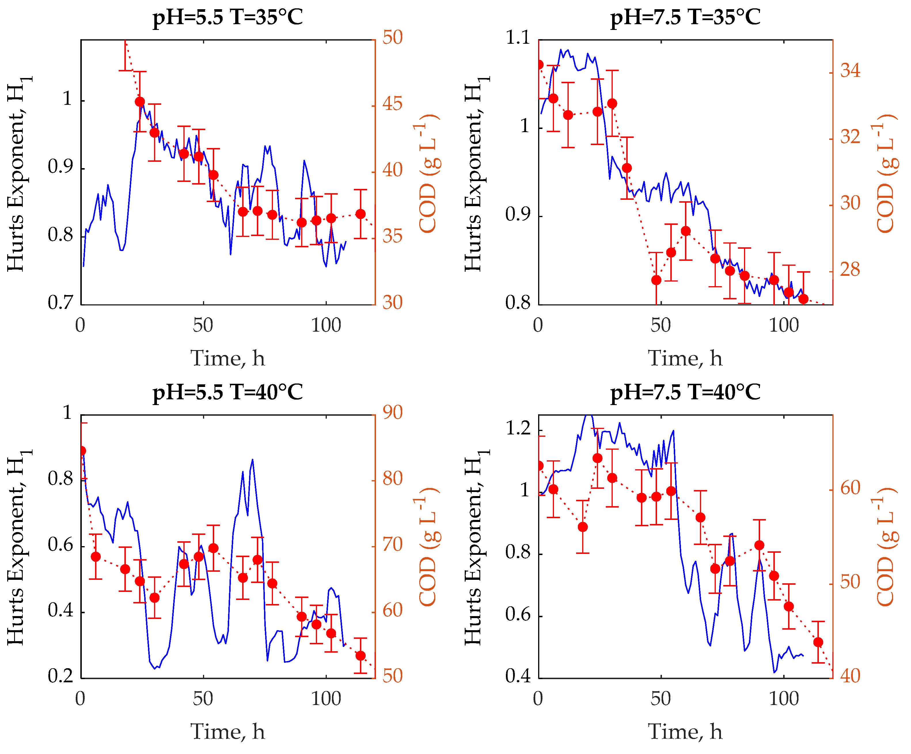
3.1. Experimental Tests

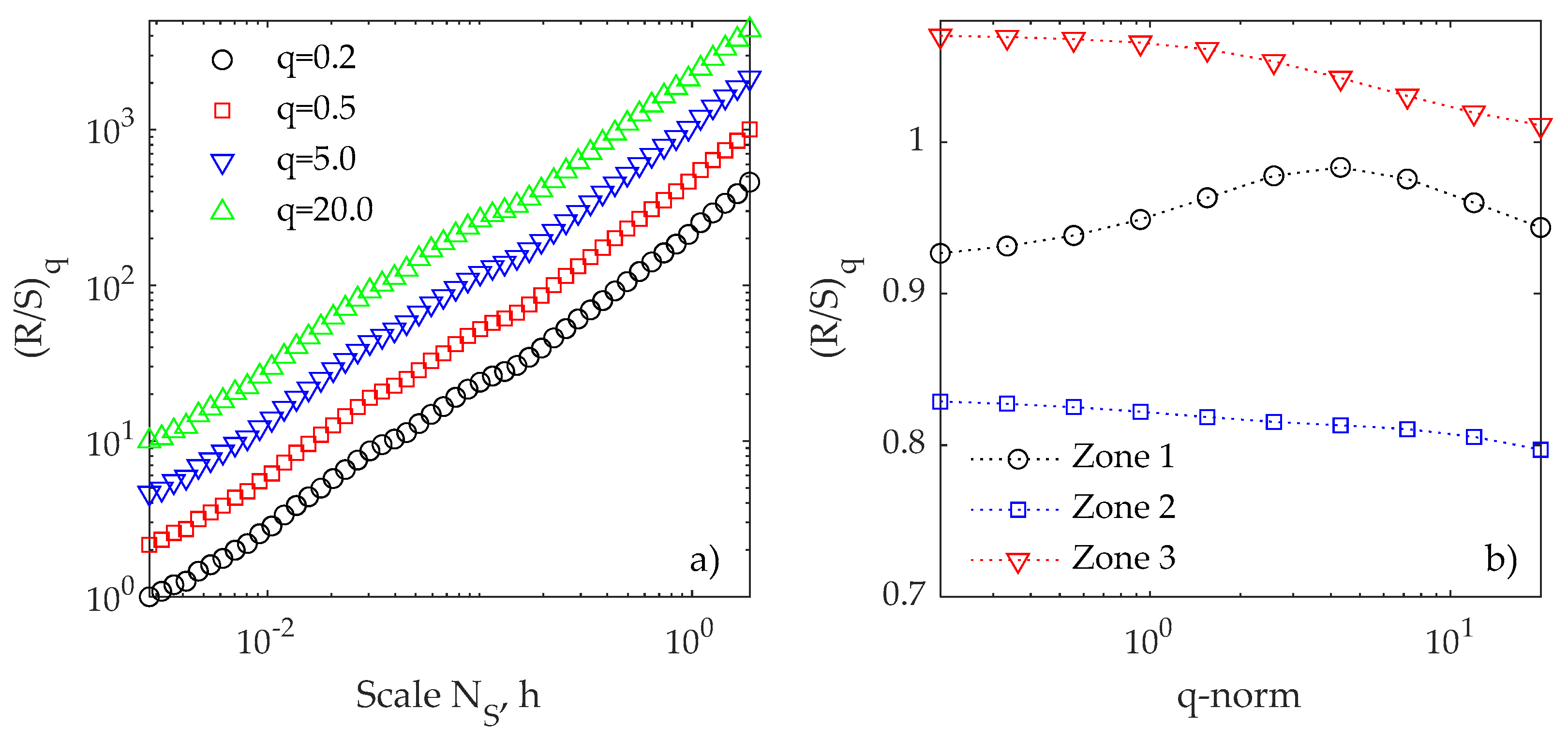
Whey is considered a complex substrate that is constituted mainly by carbohydrates, proteins, and lipids. At the conditions evaluated in this work, it is observed that total carbohydrates are consumed up to 95% in the first 35 h of operation (Figure 2).

However, the COD consumption only reaches a consumption between 30 and 50%, which suggests that the consumption of lipids and proteins was less significant. At pH = 7.5 and T = 40 °C, 50% of the COD consumption is reached, while at pH = 5.5 and T = 35 °C the minimum consumption is obtained with 30% (Figure 3). These results correspond to those obtained by Perna et al. [49], who achieved COD removal percentages between 14% and 32% using diluted whey.

Regarding VFA production, the amount and types of VFA produced mainly depend on the initial pH. In Figure 3, the production of VFA is shown, noting that at initial pH = 5.5, butyric, valeric, and caproic acids are favored. In contrast, at initial pH = 7.5, the production of acetic and propionic acids is favored. These results agree with that reported by different authors, who indicate that at pH < 6, butyric acids are favored, and at pH > 6 propionic and acetic acids are favored [50,51,52,53].

The pH time series exhibit dynamic changes that correspond to the observed changes in key process variables. For the first 35 h, where the carbohydrate consumption rate is high, the pH series shows strong fluctuations, which could indicate the high activity of hydrolytic microorganisms. Subsequently, after 40 h, the experiments at pH 5.5 present an alkalinization stage, observing an increase in pH values of 6.8–7. This behavior can be associated with the production of biogas. Indeed, the presence of CO₂ promotes the generation of bicarbonates which causes an increase in pH. For the experiments at pH = 7.5, the alkalinization stage begins at 80 h, showing a slight increase in pH, reaching a maximum value of pH = 8.3. Finally, when the pH stabilizes, the highest VFA production rate is observed, which indicates the high activity of the acidogenic-acetogenic microorganisms.

3.2. R/S Analysis

R/S analysis is applied to the pH series of the four experimental conditions. The time scale interval is given by N_S,min = 20 data (20 s) and N_S,max = 3600 data (1 h), which according to Sanchez-Garcia et al. [37], is the time scale where the characteristic phenomena corresponding to each of the stages of the anaerobic digestion of crude whey can be identified. Figure 4 shows the statistic (R/S)2 as a function of the time scale Ns, observing that the power-law ((R/S) = aNs^H) exhibits three changes in slope (i.e., three different values of the Hurst exponent, H₁, H₂, and H₃), named as Zones 1, 2, and 3. The presence of different values of the Hurst exponent suggests that the R/S analysis can identify three characteristic phenomena immersed in the fluctuations of the pH series. These zones correspond to those reported in the anaerobic digestion of whey [37] and tequila vinasse [35,36], where each region was attributed to a different anaerobic digestion stage. Based on the above observations, Zone 1 is related to hydrolysis, Zone 2 corresponds with the acidogenesis and acetogenesis stages, and Zone 3 is related to methanogenesis. It should be noted that in conventional anaerobic digestion processes, the experimental conditions favor methane-rich biogas production. In contrast, in this study, the operating conditions favor the VFA production, so the methanogenic stage is not significant.

Table 2. Hurst exponent by zone for the four experimental tests.

Zone/Test	T = 35 °C pH = 5.5	T = 35 °C pH = 7.5	T = 40 °C pH = 5.5	T = 40 °C pH = 7.5
Zone 1	0.85819	0.99983	1.01371	0.9804
Zone 2	1.12514	0.73615	0.51536	0.79128
Zone 3	1.05433	0.89266	1.28973	1.05855

shows the values of the Hurst exponent for each zone, where it is observed that the H₁ values are around 1.0, indicating that in this time scale, there are characteristic phenomena with similar behavior for all the operating conditions evaluated. On the other hand, the Hurst exponent values in Zones 2 and 3 show more significant variability between operating conditions, which indicates that the phenomena on these characteristic scales are more susceptible to changes in pH and temperature.

According to the above, Zone 1 could be correlated with the hydrolytic stage. In all experiments, the COD consumption is mainly to carbohydrate degradation, which is consumed up to 95% in the first two days. Zones 2 and 3 could be correlated with the acidogenic-acetogenic stages, which show the formation of different fatty acids depending on the operating conditions evaluated. For example, at pH = 5.5, higher production of butyric and caproic acids is obtained, while at pH = 7.5, higher production of acetic and propionic acids is obtained. Note that the H₃ value is higher when there is a more significant formation of butyric and caproic acids.

In order to identify correlations between the key variables and the Hurst exponents, the R/S analysis is implemented considering 6 h windows, which are shifted every hour, covering the whole series. This allows one to obtain the Hurst exponent values as a function of scale and time. For the four experimental conditions, Figure 5 shows the dynamic R/S analysis, where the three zones described in Figure 4 can be identified, noting that the H values show temporal variations in each zone, which can be correlated with those of the process stages.

In order to avoid different interpretations of the dynamic Hurst exponent, the average is carried out in each zone, which leads to an H dynamic profile for each zone (i.e., Hd₁, Hd_2, and Hd₃). These profiles are compared with the experimental measurements of COD and VFA.

Considering the four experimental conditions, Figure 6 shows the comparison between the COD measurements with Hd₁, where it is observed that the Hd₁ dynamic exhibits the same trend observed with the COD consumption, which confirms that the time scale of Zone 1 corresponds to the hydrolysis stage in the anaerobic treatment of whey.

Figure 7 shows the comparison between the total VFA measurements produced with the Hd₃ dynamic profile, finding that both profiles exhibit the same behavior, suggesting that the time scale of Zone 3 corresponds to the acidogenic-acetogenic stage. Hd₂ profile shows behavior that cannot be correlated with any of the process variables.

Moreover, due to the operating conditions evaluated, there is no significant methane production, so the methanogenic stage is not considered as an active stage of the process. Then, Hurst exponents dynamic could be used as qualitative indexes for monitoring the COD and VFA for different operating conditions.

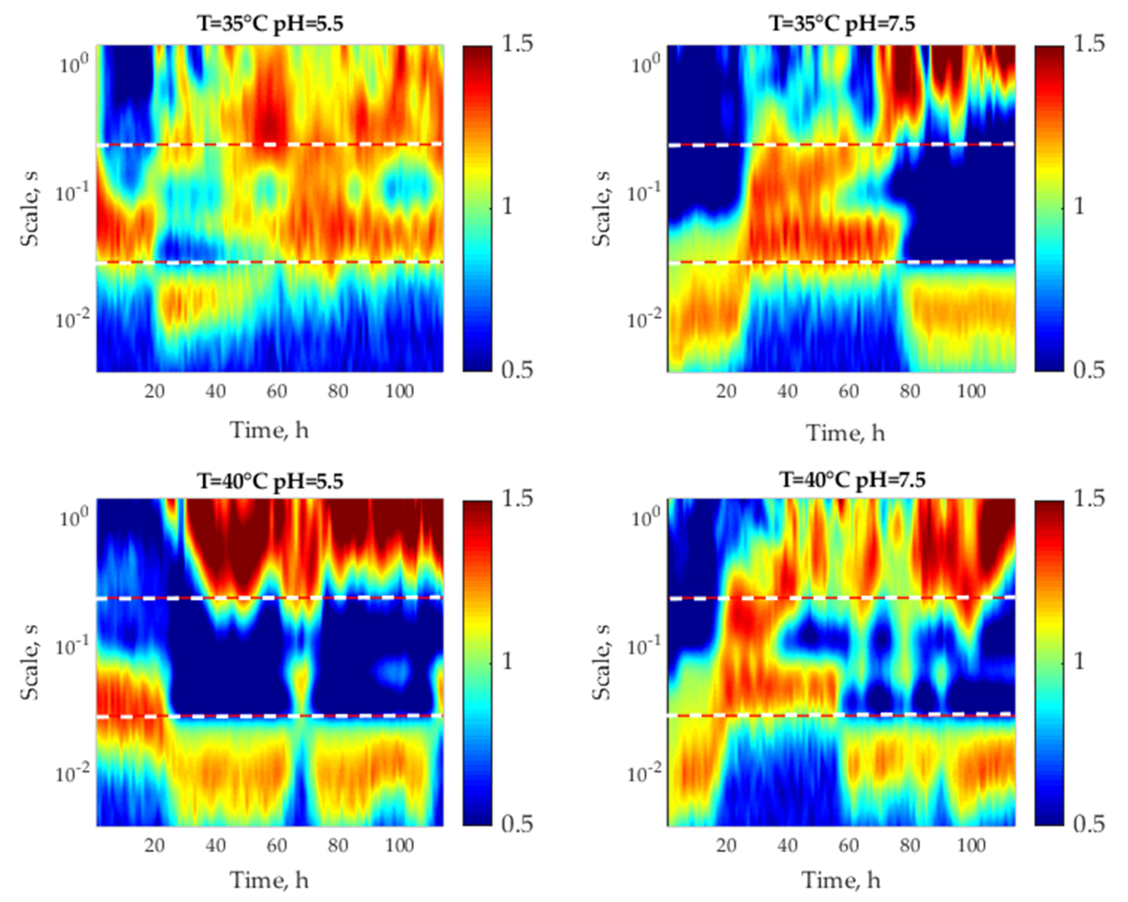
3.3. Multifractal Analysis

The multifractal analysis is a useful tool to identify information at different time scales associated with the inherent complexity in bioprocesses. The anaerobic treatment of raw cheese whey is a highly complex process involving transport phenomena and bioreactions, affecting overall process stability. This interaction depends on the evaluated operating conditions and is reflected in the type and quantity of products generated.

In Figure 8, the application of the multifractal R/S analysis is presented, considering q ∈ [0.2, 20]. For the experimental test at T = 40 °C and initial pH = 5.5, Figure 8a shows the statistic (R/S)q, noting that the slopes (H_q) of the three zones show variations at different values of q-norm. Figure 8b shows that the H_q values of the three zones present nonlinear variations with respect to the q-norm that exhibit significant differences in each zone, suggesting the presence of a multifractal behavior in the global process, as well as in each of the stages that make up the process.

The degree of multifractality of each process stage is evaluated with the multifractal index (IM). The higher the IM value, the greater the multifractal behavior.

Table 3. Multifractal index by zone for the four experimental tests.

Zone/Test	T = 35 °C pH = 5.5	T = 35 °C pH = 7.5	T = 40 °C pH = 5.5	T = 40 °C pH = 7.5
Zone 1	0.0725	0.0919	0.0469	0.1107
Zone 2	0.028	0.1929	0.0679	0.1414
Zone 3	0.0115	0.1691	0.1756	0.1039

shows the multifractal index of the three zones for the four experimental tests. The lowest values of the multifractal index correspond to Zone 1, associated with the hydrolytic stage. Regardless of the operating conditions evaluated, a similar behavior is observed in all experiments. Whereas Zone 3, associated with the acidic stage, shows the highest values of the multifractal index, which correspond to the generation of products obtained in this stage. It should be noted that different types of VFA are produced and the quantity produced depends on the operating conditions.

Globally, the multifractal index identifies which stage of the process presents more significant interactions between the underlying phenomena. In order to determine the changes in multifractality as the process is carried out, the multifractal index is calculated considering 6 h moving windows. Figure 9 shows the scale-temporal changes of the multifractal index, where it is observed that the dynamic changes of the IM correspond to the variations observed in the consumption/production rates of the key variables. In Zone 1, it is observed that the most important changes in IM occur in the first 30 h of the process, where the maximum consumption of carbohydrates is carried out. In Zone 3, more significant dynamic changes are observed associated with the changes in the VFA production rate. Increases in the IM correspond to the increases in the VFA production rate.

4. Conclusions

This work proposed the application of fractal analysis to pH time series collected from the anaerobic treatment of raw cheese whey in an anaerobic batch digester for four different operating conditions variating the pH and temperature. The rescaled range analysis identifies three regions that suggest three underlying phenomena in the anaerobic digestion treatment for raw cheese whey. The dynamic R/S analysis has permitted a qualitative description of two key variables for the four experimental sets. Thus, the R/S fractal methodology can be used as a tool for indirect monitoring of COD consumption and VFA production to different operating conditions. The fact that key variables can be monitored by pH measurements under different operating conditions is a promising advance for developing an economic diagnosis and monitoring and control system that can indicate process performance. Indeed, results in this paper can be used in conjunction with available diagnosis methods using thresholds based on VFA trends. Besides, the proposed multifractal index provides information on dynamic changes in consumption/production rates of key process variables, which are directly associated with the inherent complexity of the process.

References

1. Mockaitis, G.; Ratusznei, S.M.; Rodrigues, J.A.; Zaiat, M.; Foresti, E. Anaerobic whey treatment by a stirred sequencing batch reactor (ASBR): Effects of organic loading and supplemented alkalinity. J. Environ. Manag. 2006, 79, 198–206. [Google Scholar] [CrossRef]
2. Prazeres, A.R.; Carvalho, F.; Rivas, J. Cheese whey management: A review. J. Environ. Manag. 2012, 110, 48–68. [Google Scholar] [CrossRef]
3. Zhang, Q.; Hu, J.; Lee, D.-J. Biogas from anaerobic digestion processes: Research updates. Renew. Energy 2016, 98, 108–119. [Google Scholar] [CrossRef]
4. Ward, A.J.; Hobbs, P.J.; Holliman, P.J.; Jones, D.L. Optimisation of the anaerobic digestion of agricultural resources. Bioresour. Technol. 2008, 99, 7928–7940. [Google Scholar] [CrossRef] [PubMed]
5. Falk, H.M.; Reichling, P.; Andersen, C.; Benz, R. Online monitoring of concentration and dynamics of volatile fatty acids in anaerobic digestion processes with mid-infrared spectroscopy. Bioprocess Biosyst. Eng. 2014, 38, 237–249. [Google Scholar] [CrossRef] [PubMed]
6. Pind, P.F.; Angelidaki, I.; Ahring, B.K.; Stamatelatou, K.; Lyberatos, G. Monitoring and Control of Anaerobic Reactors. Blue Biotechnol. 2003, 82, 135–182. [Google Scholar] [CrossRef]
7. Wu, D.; Li, L.; Zhao, X.; Peng, Y.; Yang, P.; Peng, X. Anaerobic digestion: A review on process monitoring. Renew. Sustain. Energy Rev. 2019, 103, 1–12. [Google Scholar] [CrossRef]
8. Noike, T.; Endo, G.; Chang, J.-E.; Yaguchi, J.-I.; Matsumoto, J.-I. Characteristics of carbohydrate degradation and the rate-limiting step in anaerobic digestion. Biotechnol. Bioeng. 1985, 27, 1482–1489. [Google Scholar] [CrossRef]
9. Spanjers, H.; Van Lier, J. Instrumentation in anaerobic treatment—Research and practice. Water Sci. Technol. 2006, 53, 63–76. [Google Scholar] [CrossRef]
10. Madsen, M.; Holm-Nielsen, J.B.; Esbensen, K.H. Monitoring of anaerobic digestion processes: A review perspective. Renew. Sustain. Energy Rev. 2011, 15, 3141–3155. [Google Scholar] [CrossRef] [Green Version]
11. Jimenez, J.; Latrille, E.; Harmand, J.; Robles, Á.; Ferrer, J.; Gaida, D.; Wolf, C.; Mairet, F.; Bernard, O.; Alcaraz-Gonzalez, V.; et al. Instrumentation and control of anaerobic digestion processes: A review and some research challenges. Rev. Environ. Sci. Bio/Technol. 2015, 14, 615–648. [Google Scholar] [CrossRef]
12. Boe, K.; Batstone, D.J.; Steyer, J.-P.; Angelidaki, I. State indicators for monitoring the anaerobic digestion process. Water Res. 2010, 44, 5973–5980. [Google Scholar] [CrossRef]
13. Ahring, B.K.; Sandberg, M.; Angelidaki, I.J.A.M. Volatile fatty acids as indicators of process imbalance in anaerobic di-gestors. Appl. Microbiol. Biotechnol. 1995, 43, 559–565. [Google Scholar] [CrossRef]
14. Nielsen, H.B.; Uellendahl, H.; Ahring, B.K. Regulation and optimization of the biogas process: Propionate as a key pa-rameter. Biomass Bioenergy 2007, 31, 820–830. [Google Scholar] [CrossRef] [Green Version]
15. Molina, F.; Castellano, M.; García, C.; Roca, E.; Lema, J.M. Selection of variables for on-line monitoring, diagnosis, and control of anaerobic digestion processes. Water Sci. Technol. 2009, 60, 615–622. [Google Scholar] [CrossRef]
16. Gaida, D.; Wolf, C.; Meyer, C.; Stuhlsatz, A.; Lippel, J.; Bäck, T.; Bongards, M.; McLoone, S. State estimation for anaero-bic digesters using the ADM1. Water Sci. Technol. 2012, 66, 1088–1095. [Google Scholar] [CrossRef] [PubMed]
17. Tidriri, K.; Chatti, N.; Verron, S.; Tiplica, T. Bridging data-driven and model-based approaches for process fault diagnosis and health monitoring: A review of researches and future challenges. Annu. Rev. Control. 2016, 42, 63–81. [Google Scholar] [CrossRef]
18. Montiel-Escobar, J.L.; Alcaraz-González, V.; Méndez-Acosta, H.O.; González-Álvarez, V. ADM1-Based Robust Interval Observer for Anaerobic Digestion Processes. Clean Soil Air Water 2012, 40, 933–940. [Google Scholar] [CrossRef]
19. Lara-Cisneros, G.; Dochain, D. Software Sensor for Online Estimation of the VFA’s Concentration in Anaerobic Digestion Processes via a High-Order Sliding Mode Observer. Ind. Eng. Chem. Res. 2018, 57, 14173–14181. [Google Scholar] [CrossRef]
20. Dewasme, L.; Sbarciog, M.; Rocha-Cózatl, E.; Haugen, F.; Wouwer, A.V. State and unknown input estimation of an an-aerobic digestion reactor with experimental validation. Control Eng. Pract. 2019, 85, 280–289. [Google Scholar] [CrossRef]
21. Draa, K.C.; Zemouche, A.; Alma, M.; Voos, H.; Darouach, M. A Nonlinear observer-based trajectory tracking method applied to an anaerobic digestion process. J. Process. Control. 2019, 75, 120–135. [Google Scholar] [CrossRef]
22. Flores-Mejia, H.; Lara-Musule, A.; Hernández-Martínez, E.; Aguilar-López, R.; Puebla, H. Indirect Monitoring of Anaero-bic Digestion for Cheese Whey Treatment. Processes 2021, 9, 539. [Google Scholar] [CrossRef]
23. Lee, J.-W.; Hong, Y.-S.T.; Suh, C.; Shin, H.-S. Online nonlinear sequential Bayesian estimation of a biological wastewater treatment process. Bioprocess Biosyst. Eng. 2011, 35, 359–369. [Google Scholar] [CrossRef]
24. Jones, R.M.; MacGregor, J.F.; Murphy, K.L. State estimation in wastewater engineering: Application to an anaerobic process. Environ. Monit. Assess. 1989, 13, 271–282. [Google Scholar] [CrossRef] [PubMed]
25. Das, L.; Kumar, G.; Rani, M.D.; Srinivasan, B. A novel approach to evaluate state estimation approaches for anaerobic digester units under modeling uncertainties: Application to an industrial dairy unit. J. Environ. Chem. Eng. 2017, 5, 4004–4013. [Google Scholar] [CrossRef]
26. MacGregor, J.; Cinar, A. Monitoring, fault diagnosis, fault-tolerant control and optimization: Data driven methods. Comput. Chem. Eng. 2012, 47, 111–120. [Google Scholar] [CrossRef]
27. Yin, S.; Ding, S.X.; Xie, X.; Luo, H. A Review on Basic Data-Driven Approaches for Industrial Process Monitoring. IEEE Trans. Ind. Electron. 2014, 61, 6418–6428. [Google Scholar] [CrossRef]
28. Nair, V.V.; Dhar, H.; Kumar, S.; Thalla, A.K.; Mukherjee, S.; Wong, J.W. Artificial neural network based modeling to evaluate methane yield from biogas in a laboratory-scale anaerobic bioreactor. Bioresour. Technol. 2016, 217, 90–99. [Google Scholar] [CrossRef]
29. Tufaner, F.; Demirci, Y. Prediction of biogas production rate from anaerobic hybrid reactor by artificial neural network and nonlinear regressions models. Clean Technol. Environ. Policy 2020, 22, 713–724. [Google Scholar] [CrossRef]
30. Newhart, K.B.; Holloway, R.W.; Hering, A.S.; Cath, T.Y. Data-driven performance analyses of wastewater treatment plants: A review. Water Res. 2019, 157, 498–513. [Google Scholar] [CrossRef]
31. Kazemi, P.; Bengoa, C.; Steyer, J.-P.; Giralt, J. Data-driven techniques for fault detection in anaerobic digestion process. Process. Saf. Environ. Prot. 2021, 146, 905–915. [Google Scholar] [CrossRef]
32. Asadi, M.; Guo, H.; McPhedran, K. Biogas production estimation using data-driven approaches for cold region municipal wastewater anaerobic digestion. J. Environ. Manag. 2020, 253, 109708. [Google Scholar] [CrossRef]
33. Qin, S.J. Survey on data-driven industrial process monitoring and diagnosis. Annu. Rev. Control. 2012, 36, 220–234. [Google Scholar] [CrossRef]
34. Lee, H.W.; Lee, M.W.; Park, J.M. Multi-scale extension of PLS algorithm for advanced on-line process monitoring. Chemom. Intell. Lab. Syst. 2009, 98, 201–212. [Google Scholar] [CrossRef]
35. Méndez-Acosta, H.O.; Hernandez-Martinez, E.; Jáuregui-Jáuregui, J.A.; Alvarez-Ramirez, J.; Puebla, H. Monitoring anaerobic sequential batch reactors via fractal analysis of pH time series. Biotechnol. Bioeng. 2013, 110, 2131–2139. [Google Scholar] [CrossRef] [PubMed]
36. Hernandez-Martinez, E.; Puebla, H.; Mendez-Acosta, H.; Alvarez-Ramirez, J. Fractality in pH time series of continuous anaerobic bioreactors for tequila vinasses treatment. Chem. Eng. Sci. 2014, 109, 17–25. [Google Scholar] [CrossRef]
37. Sánchez-García, D.; Hernández-García, H.; Mendez-Acosta, H.O.; Hernández-Aguirre, A.; Puebla, H.; Hernández-Martínez, E. Fractal Analysis of pH Time-Series of an Anaerobic Digester for Cheese Whey Treatment. Int. J. Chem. React. Eng. 2018. [Google Scholar] [CrossRef]
38. Jirka, A.M.; Carter, M.J. Micro semiautomated analysis of surface and waste waters for chemical oxygen demand. Anal. Chem. 1975, 47, 1397–1402. [Google Scholar] [CrossRef] [PubMed]
39. Rice, E.W.; Baird, R.B. Standard Methods for the Examination of Water and Wastewater; American Water Works Association: Denver, CO, USA, 1995. [Google Scholar]
40. Dubois, M.; Gilles, K.A.; Hamilton, J.K.; Rebers, P.A.; Smith, F. Colorimetric Method for Determination of Sugars and Related Substances. Anal. Chem. 1956, 28, 350–356. [Google Scholar] [CrossRef]
41. Bradford, M.M. A rapid and sensitive method for the quantitation of microgram quantities of protein utilizing the principle of protein-dye binding. Anal. Biochem. 1976, 72, 248–254. [Google Scholar] [CrossRef]
42. Hurst, H.E. Long-Term Storage Capacity of Reservoirs. Trans. Am. Soc. Civ. Eng. 1951, 116, 770–799. [Google Scholar] [CrossRef]
43. Kantelhardt, J.W.; Zschiegner, S.A.; Koscielny-Bunde, E.; Havlin, S.; Bunde, A.; Stanley, H. Multifractal detrended fluctuation analysis of nonstationary time series. Phys. A Stat. Mech. Its Appl. 2002, 316, 87–114. [Google Scholar] [CrossRef] [Green Version]
44. Mandelbrot, B.B.; Wallis, J.R. Computer Experiments with Fractional Gaussian Noises: Part 2, Rescaled Ranges and Spectra. Water Resour. Res. 1969, 5, 242–259. [Google Scholar] [CrossRef]
45. Barabási, A.-L.; Vicsek, T. Multifractality of self-affine fractals. Phys. Rev. A 1991, 44, 2730–2733. [Google Scholar] [CrossRef]
46. Katsuragi, H.; Honjo, H. Multiaffinity and entropy spectrum of self-affine fractal profiles. Phys. Rev. E 1999, 59, 254–262. [Google Scholar] [CrossRef]
47. Xu, Y.; Qian, C.; Pan, L.; Wang, B.; Lou, C. Comparing Monofractal and Multifractal Analysis of Corrosion Damage Evolution in Reinforcing Bars. PLoS ONE 2012, 7, e29956. [Google Scholar] [CrossRef] [Green Version]
48. Sanchez-Ortiz, W.; Andrade-Gómez, C.; Hernandez-Martinez, E.; Puebla, H. Multifractal Hurst analysis for identification of corrosion type in AISI 304 stainless steel. Int. J. Electrochem. Sci. 2015, 10, 1054–1064. [Google Scholar]
49. Perna, V.; Castelló, E.; Wenzel, J.; Zampol, C.; Fontes-Lima, D.; Borzacconi, L.; Varesche, M.; Zaiat, M.; Etchebehere, C. Hydrogen production in an upflow anaerobic packed bed reactor used to treatcheese whey. Int. J. Hydrogen Energy 2013, 38, 54–62. [Google Scholar] [CrossRef]
50. Calero, R.R.; Lagoa-Costa, B.; Fernandez-Feal, M.M.D.C.; Kennes, C.; Veiga, M.C. Volatile fatty acids produc-tion from cheese whey: Influence of pH, solid retention time and organic loading rate. J. Chem. Technol. Biotechnol. Technol. 2018, 93, 1742–1747. [Google Scholar] [CrossRef]
51. Wang, K.; Yin, J.; Shen, D.; Li, N. Anaerobic digestion of food waste for volatile fatty acids (AGVs) production with different types of inoculum: Effect of pH. Bioresour. Technol. 2014, 161, 395–401. [Google Scholar] [CrossRef]
52. Lee, C.; Kim, J.; Shin, S.G.; O’Flaherty, V.; Hwang, S. Quantitative and qualitative transitions of methanogen community structure during the batch anaerobic digestion of cheese-processing wastewater. Appl. Microbiol. Biotechnol. 2010, 87, 1963–1973. [Google Scholar] [CrossRef] [PubMed]
53. Bengtsson, S.; Hallquist, J.; Werker, A.; Welander, T. Acidogenic fermentation of industrial wastewaters: Effects of chemo-stat retention time and pH on AGV production. Biochem. Eng. J. 2008, 40, 492–499. [Google Scholar] [CrossRef]
Figure 1. pH time series collected in the anaerobic treatment of raw cheese whey at different conditions of initial pH and temperature.
Applsci 11 05803 g001
Figure 2. The dynamic profile of total carbohydrate consumption.
Applsci 11 05803 g002
Figure 3. The dynamic profile of COD consumption and distribution of VFA produced.
Applsci 11 05803 g003
Figure 4. R/S statistic vs. time scale NS.
Applsci 11 05803 g004
Figure 5. Scale-temporal profile of the Hurst exponent considering a 6 h moving window.
Applsci 11 05803 g005
Figure 6. Correlations between Hd1 and COD consumption measurements.
Applsci 11 05803 g006
Figure 7. Correlations between Hd3 and VFA produced measurements.
Applsci 11 05803 g007
Figure 8. Multifractal analysis for pH time series to pH = 7.5 and T = 40 °C, (a) R/S analysis applied to different q-norm and (b) Hq as a function of q-norm.
Applsci 11 05803 g008
Figure 9. Dynamical multifractal index for two experimental tests.
Applsci 11 05803 g009