Zero Average Dynamic Controller for Speed Control of DC Motor

Abstract

This paper presents the use of the buck converter with Zero Average Dynamics to control the speed of a permanent magnet direct current motor. For this objective, we consider a fourth-order nonlinear model that describes the system’s dynamics and tests different scenarios to determine how the direct current motor responds. The results show a robust speed tracking performance of the direct current motor under the reference signal and controller parameter changes and disturbances in the load torque. A non-saturated duty cycle with fixed commutation frequency is obtained in the power supply of the DC motor, and a low steady-state value of the speed tracking error is achieved in both experimental and simulation results. In summary, the effectiveness of the Zero Average Dynamics control strategy for high order systems was experimentally proved.

1. Introduction

Power converters can efficiently transform electrical energy from the generation source to users and help meet electricity needs in the power grid [1]. In a direct current (DC) microgrid, numerous power converters are configured as interfaces between renewable energies and loads [2]. Microgrid is emerging as an efficient solution for the high integration of distributed renewable energies, energy storage systems, and flexible loads in modern power systems [3].

Digital signal processing (DSP) provides greater flexibility than analog designs [4]. Some advantages are that it provides a straightforward implementation of nonlinear controllers, quasi-sliding mode control (QSMC), and advanced control techniques [5]. Other advantages are that it provides low power consumption [6], reduces the use of external passive elements, gives low sensitivity to parameter changes, and allows various configuration options in pulse width modulation (PWM) [7,8]. However, quantization and discretization can cause periodic bands [9], chaotic behavior, oscillations, subharmonics, and limit cycles [10]. Additionally, the time delays in the output of the controllers can produce instability [11]. Thus, the performance of a well-designed discretized quasi-sliding mode control (DQSMC) may be affected when executed by a digital controller [12] due to the finite sampling frequency. Nevertheless, research on DQSMC is overly limited [13].

Authors in [10] expose the limit cycles in power electronic converters controlled with DPWM (Digital Pulse Width Modulation). They propose some conditions on the control law and the quantization limits to avoid such oscillations. The Fixed Point Inducting Control (FPIC) technique helps stabilize orbits and chaos [14], and the parameters of the power converter can be estimated as presented in [15,16]. The minimum sampling time and quantization resolution criteria for digital controller parameters have been established in [17].

Research has been conducted since the 1990s related to chaotic behavior in electric motors. For instance, some research papers have been presented that show stabilization of such chaotic behaviors [18]. Recently, techniques such as Zero Average Dynamics (ZAD) and FPIC haves been used to control DC motors, as presented in [19,20]. The FPIC technique allows researchers to reduce chaos and maintain a low error; however, the system is not robust and the steady-state error increases when internal parameters change [21]. The ZAD control technique has been validated in [22], both for the pulse to the center and pulse to the side. The author in [21] also proposed using the FPIC control technique to control chaotic systems applied to a DC-DC converter and DC-AC [23].

ZAD has been used to regulate different types of systems. For example, in [24], a dynamic sliding surface is used for the ZAD control technique as an alternative in a quasi-sliding mode. The control with ZAD has also been used to implement a buck converter in a Field Programmable Gate Array (FPGA) [25], applying ZAD with a pulse on the side fulfills the requirement of fixed switching frequency [26,27]. Additionally, studies on the transition from periodicity to chaos in a buck DC-DC converter operated with the ZAD control technique have been carried out in [28,29,30], revealing bifurcations due to period-doubling and corner collision, as well as chaotic phenomena, chaotic bands, and their doubling. Power converters help regulate the speed of DC motors to perform high-precision tasks [31]. However, some chaotic behavior in motor speed requires special control to regulate variations and maintain the motors operating efficiently.

Advanced control methods, e.g., sliding mode control (SMC) and predictive control, allow effective motor control, with high output tracking accuracy, disturbance rejection capability, and fast response. Predictive control comprises establishing a predictive model to predict future output values, the definition of a cost function in terms of the output error, and the minimization of the cost function to determine the optimal control sequence. In [32], a predictive control based on a deadbeat control algorithm is proposed for a permanent magnet synchronous motor (PMSM). An improved deadbeat control scheme is proposed in order to provide robustness and improve the motor current tracking while suppressing torque ripple. In Trivedi [33], deadbeat, hysteresis based and finite-control set methods of predictive control are proposed for a PM BLDC motor in the stationary plane. In [34], a predictive control is proposed for a long-stroke planar motor for high-precision positioning applications, considering long-stroke, time-varying trajectory tracking. An additional term is introduced to the cost function. The sliding mode control (SMC) method is designed to cope with parameter variation, model uncertainties, and disturbances. In [35], a time-dependent, global, non-singular, and fixed-time terminal SMC is proposed for a second order PMSM using a time-dependent terminal sliding surface and a piecewise continuous SMC law. In [36], an SMC is designed for a PMSM drive using an improved exponential reaching law to solve the chattering problem while providing a quick output response. In [37], an SMC is proposed for the speed control of a permanent magnet linear synchronous motor (PMLSM) using a power function in the SMC strategy to suppress the conventional SMC chattering. In motor control strategies, function approximation methods, e.g., neural networks, allow approximating of the unknown nonlinear function of the dynamic model. In [38], a neural network non-singular fast terminal SMC is proposed for a PMLSM. In [39], a neural network learning adaptive robust control (NNLARC) is proposed for an industrial linear motor-driven stage.

However, the ZAD control strategy has significant advantages in controlling power converters and drives, such as low stationary-state error, fixed commutation frequency, and non-saturated cycle. Therefore, in this paper, a ZAD control strategy is proposed for speed motor control of a converter-motor system. The experimental test of the buck converter driving the motor was built, and simulations were also performed.

The main contributions of this paper are:

• A ZAD control strategy was proposed to achieve proper tracking performance in experiments and simulations, obtaining similar results in both.
• A converter prototype was built to control the DC motor speed. This controller achieved low acoustic noise and low electromagnetic interference. In addition, it provided the possibility of defining the parameters and changing sampling frequency, switching frequency, and quantization levels of the measurements.
• A discrete quasi-sliding mode control was used to perform a fixed commutation frequency. Thus, the voltage and current values entering the motor are less abrupt.
• A versatile prototype was developed that uses different commutation frequencies, real-time parameter variation, and current and voltage measurements during a given time by using a trigger signal.

The paper is organized as follows. The mathematical model and the control technique are presented in Section 2. The numerical simulation and experimental results of the buck converter with the DC motor (buck-motor system) using the ZAD technique are included in Section 3. Finally, conclusions are presented in Section 4.

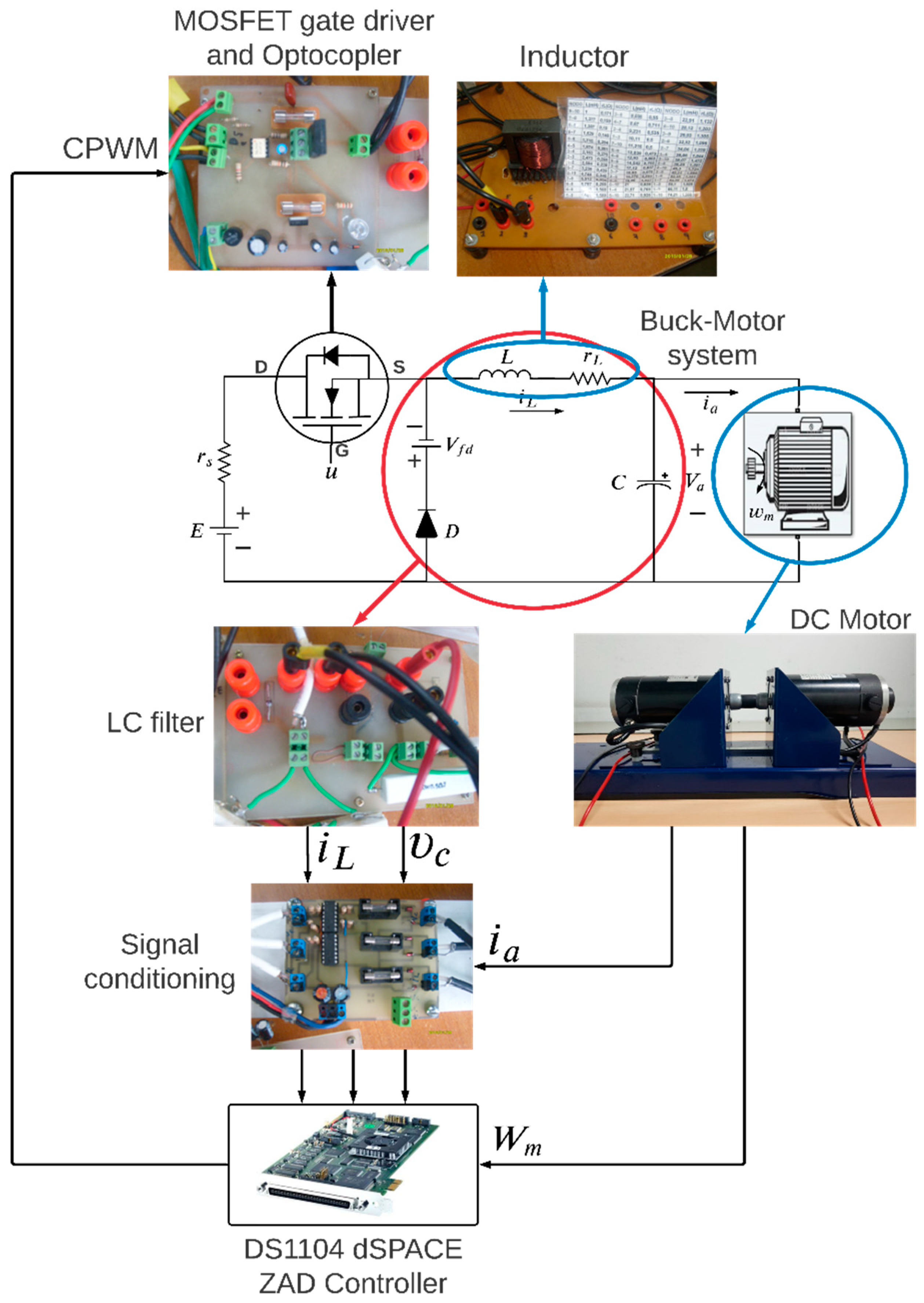
2. Materials and Methods

Figure 1 presents the diagram of the ZAD applied to the buck converter when it is used to control a DC motor. This figure shows two main blocks that were broken into the buck-motor system and the controller board. Thus, the buck converter controls the speed of the motor, the sensors measure the signals in the buck-motor system, and the gates receive the signals from the software. The controller system is composed of the blocks such as A/D inputs to obtain the signals, the ZAD controller, the input parameters, the reference signal, and CPWM that transmit the signal output to the buck-motor system.

The permanent magnet DC motor parameters are as follows: 250 W (nominal power), 42 VDC (input voltage), 6 A (current), and 4000 RPM (speed). The speed of the motor ($W_m$) is measured with an encoder of 1000 pulses per turn, ${\upsilon }_c$ is the capacitor voltage that feeds the motor, $i_L$ is the inductor current, and $i_a$ is the armature current. The controller was implemented in the dSPACE DS1104 [40,41]; therefore, the signals are sampled by the card during the real-time operation, and the output of the control is applied to the buck converter.

One fast response optocoupler (HCPL-J312) was used to isolate the card from the power grid. This device connects the control output, operates the buck converter switch, and closes the control loop.

Moreover, ${\upsilon }_c$, $i_L$, and $i_a$ pass through the 12-bit ADC inputs, the controlled variable $W_m$ is sensed by an encoder, and the variables are sensed at a sampling frequency of 6 kHz. The DC motor, buck converter, and ZAD technique control parameters are stored as constants in the control block. The DS1104 card microprocessors generate the duty cycle $d$ and the corresponding CPWM signal for the solid-state switch S with a resolution of 10 bits during each sampling time.

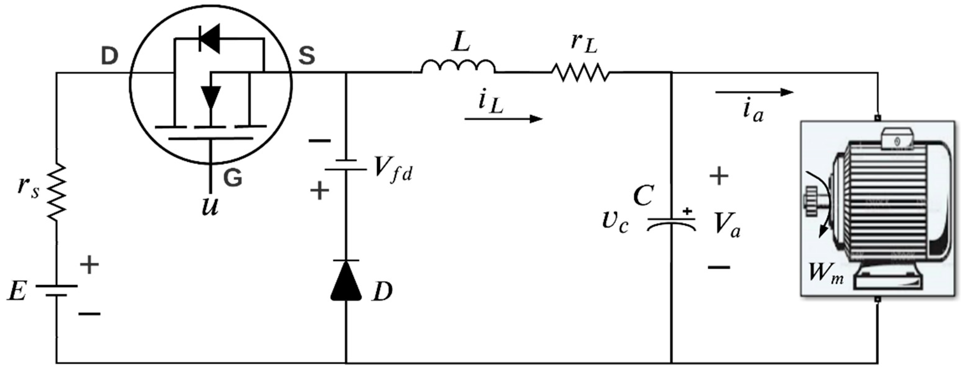
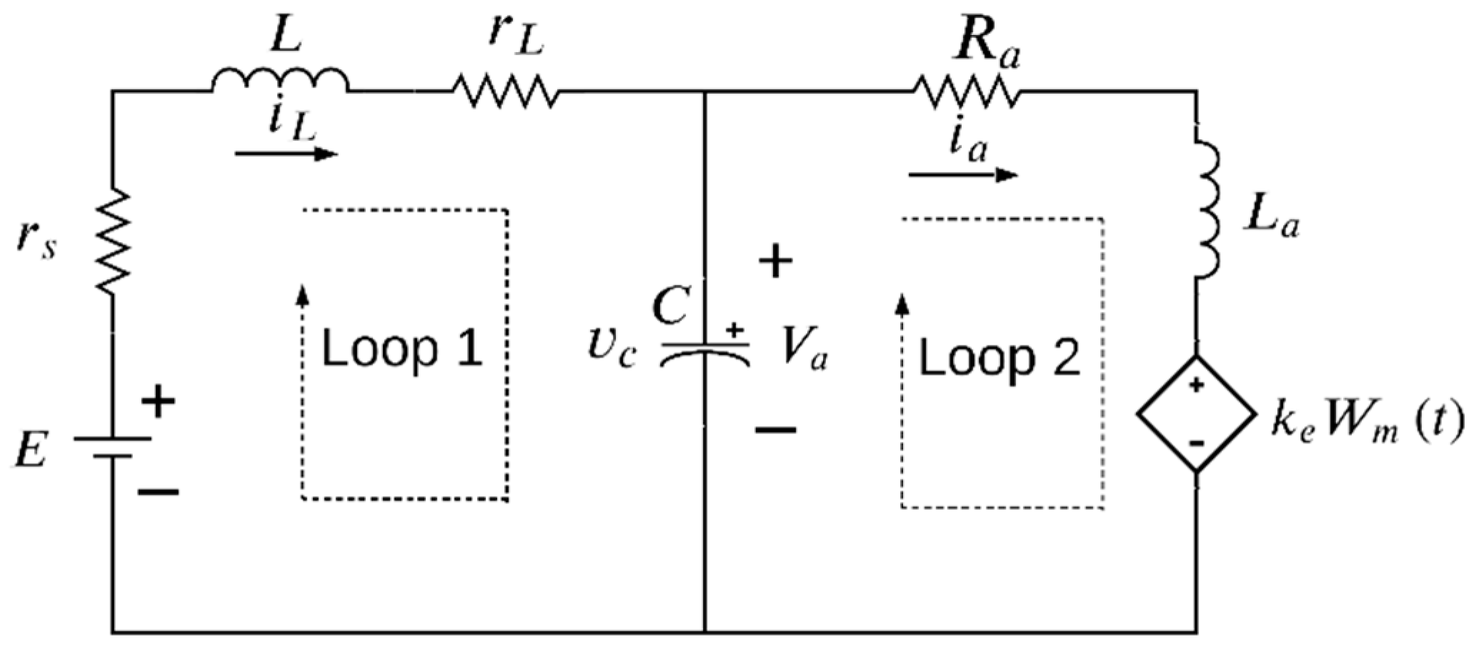
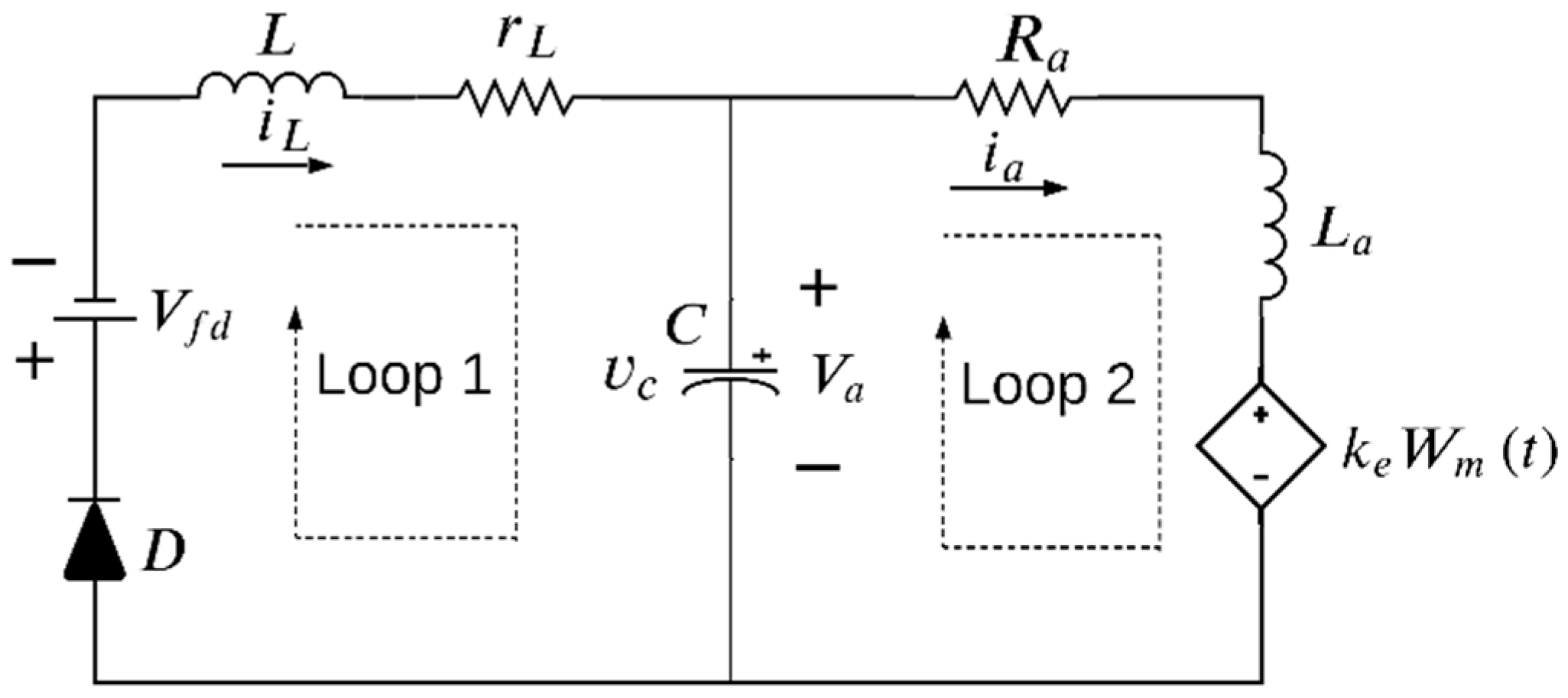
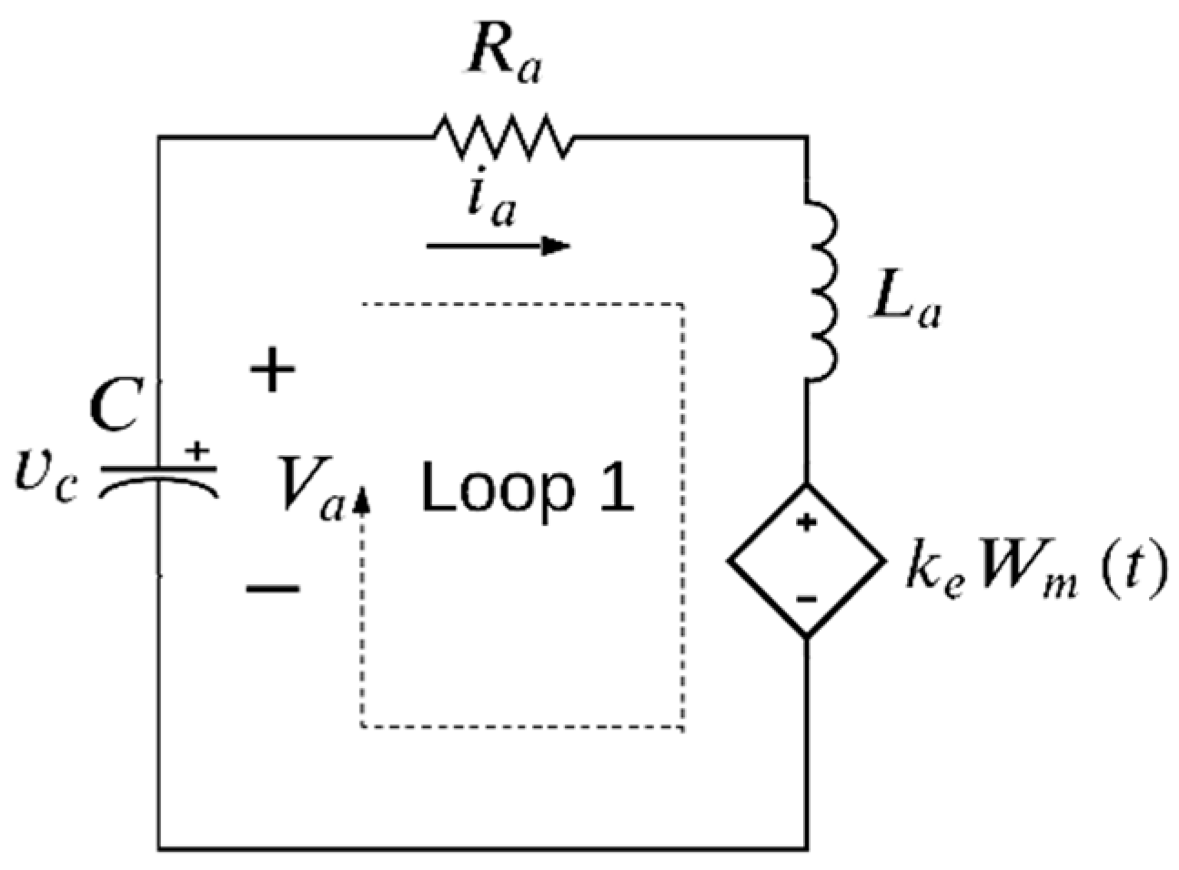
2.1. Buck-Motor System Model

The DC motor must be modeled to represent the complete circuit of the study. Consequently, the mechanical part of the model is represented in (1), and the electrical part is represented in (2). This constitutes a second-order system with some variables defined in the model, such as the speed of the motor and the armature current.

$${\dot{W}}_m\left(t\right)=\frac{-B{W}_m\left(t\right)}{J_{eq}}+\frac{k_t{i}_a\left(t\right)}{J_{eq}}+\frac{-T_{fric}}{J_{eq}}+\frac{-T_L}{J_{eq}}$$

(1)

$$\dot{i_a}\left(t\right)=\frac{-k_e}{L_a}{W}_m\left(t\right)+\frac{-R_a}{L_a}{i}_a\left(t\right)+\frac{V_a\left(t\right)}{L_a}$$

(2)

The term $R_a$ is the armature resistance (Ω) of the DC motor, $i_a\left(t\right)$ is the armature current [A], $W_m\left(t\right)$ is the speed of the motor [rad/s], $k_e$ is a voltage constant [V/rad/s], and $L_a$ is the armature inductance [mH]. Furthermore, $V_a\left(t\right)={\upsilon }_c\left(t\right)$ represents the voltage applied to the motor (V), $B$ the viscous friction coefficient (N·m/rad/s), $J_{eq}$ is the inertia moment (kg·m²), $k_t$ is the torque constant of the motor (N·m/A), $T_{fric}$ is the friction torque (N·m), and $T_L$ is the load torque (N·m). These parameters were measured and calibrated in real time using a dSPACE board and the method described in [42].

Figure 2 illustrates the diagram of the buck-motor system. This model considers the following terms: $E$ as the source voltage, $r_s$ the internal source resistance, $D$ as the diode, $C$ as the capacitor, $L$ as the inductor, $r_L$ the inductor resistance, and $V_{fd}$ as the forward voltage of the diode. Other previously defined variables used in this model are $W_m$ as the speed of the motor [rad/s], $i_a$ is the armature current [A], $V_a$ represents the voltage applied to the motor (V).

The advantages of using this converter to feed the DC motor are defined as follows. The system protects the motor because there are no sudden voltage and current changes at the input. Besides, it provides a regulated voltage and prevents overheating, increasing its useful life.

According to the operation of this system, a better study can be performed with circuits broken down into two parts, as in Figure 3 and Figure 4. For instance, Figure 3 shows the equivalent circuit for a continuous conduction mode when the switch S = ON and the diode is inactive. The second part of the circuit is presented when the diode is on conduction and the switch opens (S = OFF), as shown in Figure 4.

If Kirchhoff’s laws are applied to the circuit in Figure 3, the model is then represented as in Equation (3). This is a complete form that represents $\dot{x}=A_{1}x+B_1$ after considering that the variables in Equation (3) are presented as $x_1=W_m$, $x_2=i_a$, $x_3={\upsilon }_c$, and $x_4=i_L$.

$$\left[\begin{array}{c}{\dot{W}}_m\\ {\dot{i}}_a\\ \dot{{\upsilon }_c}\\ \dot{i_L}\end{array}\right]=\left[\begin{array}{cccc}\frac{-B}{J_{eq}}& \frac{k_t}{J_{eq}}& 0& 0\\ \frac{-k_e}{L_a}& \frac{-R_a}{L_a}& \frac{1}{L_a}& 0\\ 0& \frac{-1}{C}& 0& \frac{1}{C}\\ 0& 0& \frac{-1}{L}& \frac{-\left(r_L+r_s\right)}{L}\end{array} \right]\left[\begin{array}{c}{W}_m\\ i_a\\ {\upsilon }_c\\ i_L\end{array}\right]+\left[\begin{array}{c}\frac{-\left(T_{fric}+T_L\right)}{J_{eq}}\\ 0\\ 0\\ \frac{E}{L}\end{array}\right]$$

(3)

The electrical circuit presented in Figure 4, when the switch S is open ($S=OFF$), can be modeled as in Equation (4). This is a complete form that represents $\dot{x}=A_{2}x+B_2$ after considering that the variables in Equation (4) are presented as $x_1=W_m$, $x_2=i_a$, $x_3={\upsilon }_c$, and $x_4=i_L$.

$$\left[\begin{array}{c}{\dot{W}}_m\\ {\dot{i}}_a\\ \dot{{\upsilon }_c}\\ \dot{i_L}\end{array}\right]=\left[\begin{array}{cccc}\frac{-B}{J_{eq}}& \frac{k_t}{J_{eq}}& 0& 0\\ \frac{-k_e}{L_a}& \frac{-R_a}{L_a}& \frac{1}{L_a}& 0\\ 0& \frac{-1}{C}& 0& \frac{1}{C}\\ 0& 0& \frac{-1}{L}& \frac{-\left(r_L\right)}{L}\end{array} \right]\left[\begin{array}{c}{W}_m\\ i_a\\ {\upsilon }_c\\ i_L\end{array}\right]+\left[\begin{array}{c}\frac{-(T_{fric}+T_L)}{J_{eq}}\\ 0\\ 0\\ \frac{-V_{fd}}{L}\end{array}\right]$$

(4)

A fourth-order system, presented in (3) and (4), considers the state variables such as $W_m$, $i_a$, ${\upsilon }_c$, and $i_{L.}$ The capacitance and inductance of the converter are denoted by the parameters $C$ and $L$, respectively. The internal source resistance is summed with the parasitic resistance of the MOSFET to obtain the total parasitic resistance as $r_s$. Besides, to obtain the total inductor resistance, the coil resistance and the measurement resistance are summed as in $r_L$. Then, $V_{fd}$ is the forward voltage of the diode, the power supply is denoted as $E$, and the value that energizes the buck-motor system depends on the state of the switch S controlled by the pulses of the CPWM signal ($E$ with S is ON or $V_{fd}$ with S is OFF).

The same circuit that considers a buck-motor system can also be represented in the discontinuous conduction mode, which occurs when the switch S is open and $i_L\le 0$. As a result, the diode in Figure 2 is in reverse conduction and the circuit is reduced, as seen in Figure 5. Now, the differential equation presented in (5) is obtained and it can also be expressed in a simple form as $\dot{x}=A_{MCD}x+B_{MCD}$. Herein, the variables $x_1=W_m$, $x_2=i_a$, $x_3={\upsilon }_c$, and $x_4=i_L$.

$$\left[\begin{array}{c}{\dot{W}}_m\\ {\dot{i}}_a\\ \dot{{\upsilon }_c}\\ \dot{i_L}\end{array}\right]=\left[\begin{array}{cccc}\frac{-B}{J_{eq}}& \frac{k_t}{J_{eq}}& 0& 0\\ \frac{-k_e}{L_a}& \frac{-R_a}{L_a}& \frac{1}{L_a}& 0\\ 0& \frac{-1}{C}& 0& 0\\ 0& 0& 0& 0\end{array} \right]\left[\begin{array}{c}{W}_m\\ i_a\\ {\upsilon }_c\\ i_L\end{array}\right]+\left[\begin{array}{c}\frac{-(T_{fric}+T_L)}{J_{eq}}\\ 0\\ 0\\ 0\end{array}\right]$$

(5)

The following step is used to configure the CPWM to send a signal with a pulse to the center. Additionally, the buck converter is configured to work in continuous conduction mode. The dynamic response of the system in a complete period can be written as in Equation (6):

$$\dot{x}=\{\begin{array}{l}{A}_{1}x+B_1 if kT\le t\le kT+dT/2\\ A_{2}x+B_2 if kT+dT/2<t<kT+T-dT/2\\ A_{1}x+B_1 if kT+T-dT/2<t<kT+T\end{array}$$

(6)

The state derivative, named as $\dot{x}$, is obtained using Equation (7). Herein, the term $k$ is the $k\mathrm{th}$ iteration of the system with a switching period $T$.

$$\dot{x}={\left[{\dot{x}}_1,{\dot{x}}_2,{\dot{x}}_3,{\dot{x}}_4\right]}^t\equiv {[\frac{d{x}_1}{dt},\frac{d{x}_2}{dt},\frac{d{x}_3}{dt},\frac{d{x}_4}{dt}]}^t\equiv {[\frac{d{W}_m}{dt},\frac{d{i}_a}{dt},\frac{d{\upsilon }_c}{dt},\frac{d{i}_L}{dt}]}^t$$

(7)

2.2. Solution of the Buck-Motor System

First, the buck converter was set to work in continuous conduction mode. In this case, the solution is presented as follows

$$x \left(t\right)=\{\begin{array}{l}{e}^{A_{1}t}{M}_1-V_1 if kT\le t\le \left(k + d/2\right) T\\ e^{A_{2}t}{M}_2-V_2 if \left(k + d/2\right) T <t <\left(k + 1-d/2\right) T \\ e^{A_{1}t}{M}_3-V_1 if \left(k + 1-d/2\right) T\le t\le \left(k + 1\right) T\end{array}$$

(8)

where the terms related to $M_1$, $M_2$, and $M_3$ are calculated as follows

$$M_1=x \left(0\right)+V_1$$

(9)

$$M_2=Q_{12}{M}_1-{\Delta }V{e}^{-A_{2}T\frac{d}{2}}$$

(10)

$$M_3=Q_{21}{M}_2+{\Delta }V{e}^{-A_{1}T \left(1-\frac{d}{2}\right)}$$

(11)

being the terms $Q_{12}$ and $Q_{21}$ defined as follows

$$Q_{12}=e^{\left(A_1-A_2\right)T \left(\frac{d}{2}\right)}$$

(12)

$$Q_{21}=e^{\left(A_2-A_1\right)T \left(1-\frac{d}{2}\right)}$$

(13)

and the three terms $V_1$, $V_2$, and ${\Delta }V$ used in previous equations are calculated as follows

$$V_1=A_1^{-1}{B}_1$$

(14)

$$V_2=A_2^{-1}{B}_2$$

(15)

$${\Delta }V=V_1-V_2$$

(16)

The solution for discontinuous conduction mode obtained is presented next:

$$x \left(t\right)=e^{A_{MCD}t}\left[x \left(0\right)+A_{MCD}^{-1}{B}_{MCD}\right]-A_{MCD}^{-1}{B}_{MCD}$$

(17)

Starting from the continuous-time solution given in Equation (8) and discretizing the output signals for each sampling period T, the continuous conduction mode solution for the buck-motor system is represented as follows:

$$\left(\left(k+1\right)T\right)=e^{A_{1}T}Qx\left(kT\right)+e^{A_{1}T}Q{V}_1-Q_{12}{e}^{A_{2}T \left(1-\frac{d}{2}\right)}{\Delta }V+e^{A_{1}T\frac{d}{2}}{\Delta }V-V_1$$

(18)

The term Q can be obtained using Equation (19):

$$Q=e^{\left(A_2-A_1\right) T}{e}^{\left(A_1-A_2\right) Td}$$

(19)

Finally, a solution is obtained in discrete time as in Equation (20):

$$x\left(\left(k+1\right)T\right)=e^{A_{MCD}T}\left[x\left(kT\right)+A_{MCD}^{-1}{B}_{MCD}\right]-A_{MCD}^{-1}{B}_{MCD}$$

(20)

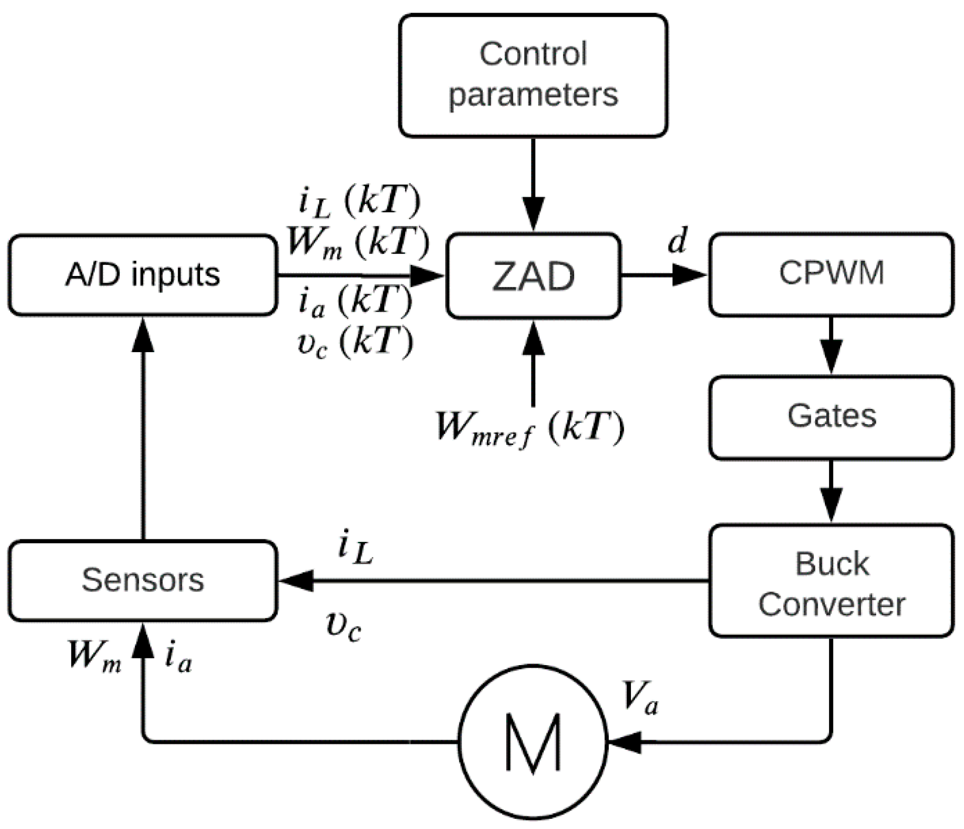
2.3. Strategy for Speed Control in a DC Motor

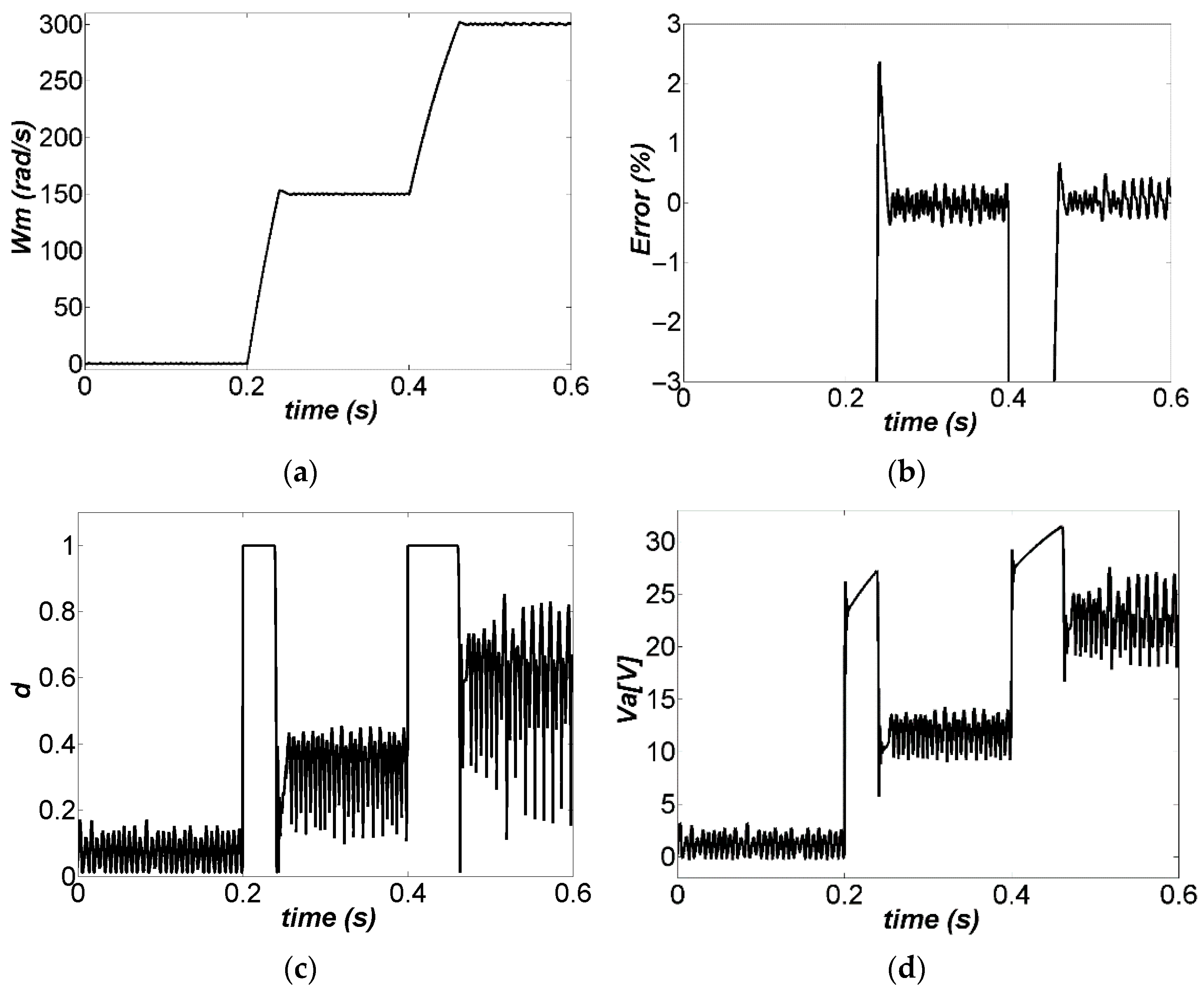
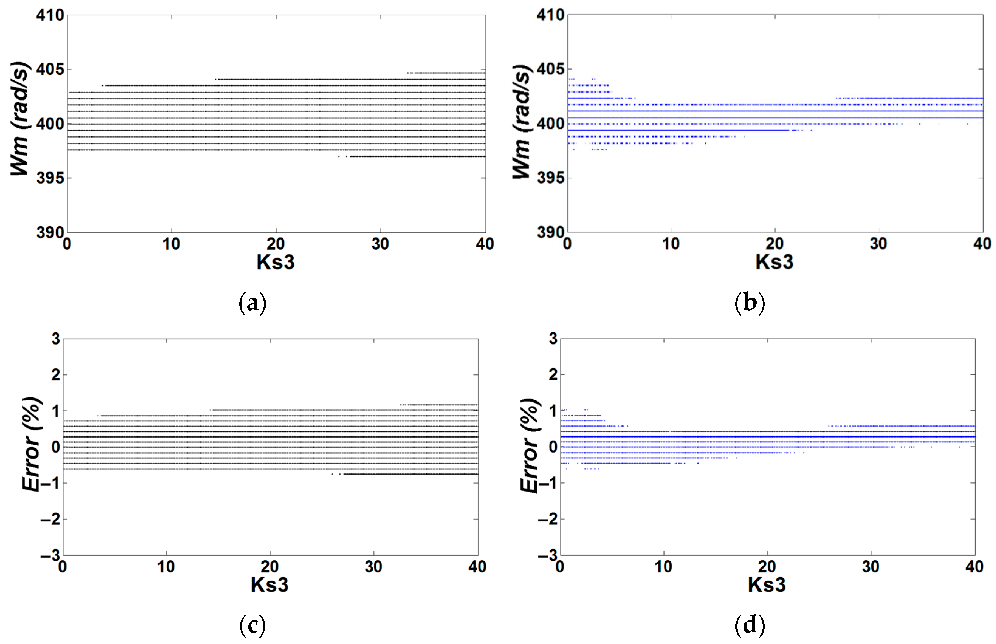
As this research aims to control the speed $W_m$, so the reference speed $W_{mref}$ must be followed and applied to the rotating load of the system. To do this in the $kT$ period, the following error is defined in the form:

$$e \left(kT\right)=W_m\left(kT\right)-W_{mref}\left(kT\right)$$

(21)

In this case, the function $s\left(x\right)$ [26] defines a third-order dynamic in the error variable, as expressed in Equation (22)

$$s\left(kT\right)=e\left(kT\right)+k_{s1}\frac{de\left(kT\right)}{d\left(kT\right)}+k_{s2}\frac{d^{2}e\left(kT\right)}{d{\left(kT\right)}^2}+k_{s3}\frac{d^{3}e\left(kT\right)}{d{\left(kT\right)}^3}$$

(22)

where the constants $k_{s1}, k_{s2}, k_{s3}$ are parameters obtained as a function of the LC filter constant multiplied by factors $K_{S1}, K_{S2}, K_{S3}$ as shown in Equation (23):

$$\begin{gathered} k_{s1}=K_{S1}\sqrt{LC} \\ {k}_{s2}=K_{S2}LC \\ {k}_{s3}=K_{S3}LC\sqrt{LC} \end{gathered}$$

(23)

In the previous equations, the terms $K_{S1}$, $K_{S2}$, and $K_{S3}$ are parameters of the ZAD. They can be considered to construct dimensional branching diagrams. Their values can be determined to achieve a desired dynamic behavior in a closed-loop system. Now, when $W_{mref}$ is constant, then Equation (22) can be written as in Equation (24) and its first derivative as Equation (25):

$$s\left(kT\right)=W_m\left(kT\right)-W_{mref}\left(kT\right)+k_{s1}\frac{d{W}_m\left(kT\right)}{d\left(kT\right)}+k_{s2}\frac{d^2{W}_m\left(kT\right)}{d{\left(kT\right)}^2}+k_{s3}\frac{d^3{W}_m\left(kT\right)}{d{\left(kT\right)}^3}$$

(24)

$$\dot{s}\left(kT\right)=\frac{d{W}_m\left(kT\right)}{d\left(kT\right)}+k_{s1}\frac{d^2{W}_m\left(kT\right)}{d{\left(kT\right)}^2}+k_{s2}\frac{d^3{W}_m\left(kT\right)}{d{\left(kT\right)}^3}+k_{s3}\frac{d^4{W}_m\left(kT\right)}{d{\left(kT\right)}^4}$$

(25)

The duty cycle is then calculated as expressed in:

$$d_k\left(kT\right)=\frac{2s \left(kT\right)+T{\dot{s}}_{-}\left(kT\right)}{T \left({\dot{s}}_{-}\left(kT\right)-{\dot{s}}_{+}\left(kT\right)\right)}$$

(26)

The term $s \left(kT\right)$ is calculated with Equation (22) at the beginning of each switching period to finally obtain $s \left(kT\right)=s \left(kT\right)|{ }_{S=ON}$. Additionally, ${\dot{s}}_{+}\left(kT\right)$ is calculated with Equation (25) to obtain ${\dot{s}}_{+}\left(kT\right)=\dot{s}\left(kT\right)|{ }_{S=ON}.$ The steps necessary to calculate these variables are shown below:

$$\begin{gathered} \frac{d{i}_L}{dt}=-\frac{1}{L}{\upsilon }_c-\frac{\left(r_s+r_L\right)}{L}{i}_L+\frac{E}{L} \\ \frac{d{\upsilon }_c}{dt}=-\frac{1}{C}{i}_a+\frac{1}{C}{i}_L \\ \frac{d{i}_a}{dt}=-\frac{k_e}{L_a}{W}_m-\frac{R_a}{L_a}{i}_a+\frac{1}{L_a}{\upsilon }_c \\ \frac{d{W}_m}{dt}=-\frac{B}{J_{eq}}{W}_m+\frac{k_t}{J_{eq}}{i}_a-\frac{\left(T_{fric}+T_L\right)}{J_{eq}} \end{gathered}$$

(27)

The second derivatives can be obtained with the previous expression and the following expression is obtained:

$$\begin{gathered} \frac{d^2{\upsilon }_c}{d{t}^2}=-\frac{1}{C}\frac{d{i}_a}{dt}+\frac{1}{C}\frac{d{i}_L}{dt} \\ \frac{d^2{i}_a}{d{t}^2}=-\frac{k_e}{L_a}\frac{d{W}_m}{dt}-\frac{R_a}{L_a}\frac{d{i}_a}{dt}+\frac{1}{L_a}\frac{d{\upsilon }_c}{dt} \\ \frac{d^2{W}_m}{d{t}^2}=-\frac{B}{J_{eq}}\frac{d{W}_m}{dt}+\frac{k_t}{J_{eq}}\frac{d{i}_a}{dt} \end{gathered}$$

(28)

The new expressions can be obtained from the second derivatives by deriving again, as shown in Equation (28).

$$\begin{gathered} \frac{d^3{i}_a}{d{t}^3}=-\frac{k_e}{L_a}\frac{d^2{W}_m}{d{t}^2}-\frac{R_a}{L_a}\frac{d^2{i}_a}{d{t}^2}+\frac{1}{L_a}\frac{d^2{\upsilon }_c}{d{t}^2} \\ \frac{d^3{W}_m}{d{t}^3}=-\frac{B}{J_{eq}}\frac{d^2{W}_m}{d{t}^2}+\frac{k_t}{J_{eq}}\frac{d^2{i}_a}{d{t}^2} \end{gathered}$$

(29)

Then, after finding a new derivate, the following expression is found:

$$\frac{d^4{W}_m}{d{t}^4}=-\frac{B}{J_{eq}}\frac{d^3{W}_m}{d{t}^3}+\frac{k_t}{J_{eq}}\frac{d^3{i}_a}{d{t}^3}$$

(30)

Applying Equations (24) and (25), and replacing with the values given by Equations (27)–(30), then, the values of $s \left(kT\right)$, $\dot{s}\left(kT\right)$ and ${\dot{s}}_{+}\left(kT\right)=\dot{s}\left(kT\right)|{ }_{S=ON}$ are obtained, where $S=ON$ means that the switch is on. On the other side, ${\dot{s}}_{-}\left(kT\right)$ is obtained from the first to the fourth derivatives with system given in (4), thus ${\dot{s}}_{-}\left(kT\right)=\dot{s}\left(kT\right)|{ }_{S=OFF}$, where $S=OFF$ means that the switch is off.

Without a delay period in the control action, the new duty cycle controlled with the ZAD technique is calculated as in Equation (31). Otherwise, with a delay period in the control action, the new duty cycle controlled with the ZAD technique is calculated as in Equation (32).

$$d_{ZAD}\left(kT\right)=\frac{2s \left(kT\right)+T{\dot{s}}_{-}\left(kT\right)}{T \left({\dot{s}}_{-}\left(kT\right)-{\dot{s}}_{+}\left(kT\right)\right)}$$

(31)

$$d_{ZAD}\left(\left(k-1\right)T\right)=\frac{2s \left(\left(k-1\right)T\right)+T{\dot{s}}_{-}\left(\left(k-1\right)T\right)}{T \left({\dot{s}}_{-}\left(\left(k-1\right)T\right)-{\dot{s}}_{+}\left(\left(k-1\right)T\right)\right)}$$

(32)

Thus, the real physical limits of the duty cycle between 0 and 1 is considered with the saturation function as follows:

$$d= \{\begin{array}{c}{d}_{ZAD}\left(\left(k-1\right)T\right) if 0<d_{ZAD}\left(\left(k-1\right)T\right)<1 \\ 1 if 1\le d_{ZAD}\left(\left(k-1\right)T\right)\\ 0 if d_{ZAD}\left(\left(k-1\right)T\right) \le 0\end{array}$$

(33)

3. Results

In this section, the performance of the buck-motor system using the ZAD technique is discussed. The parameters of the converter, motor, and control systems are shown in

Table 1. Parameters of the buck-motor system and the controller.

Parameter	Description	Value
$B$	Viscous friction coefficient	0.000138 (Nm/rad/s)
$C$	Capacitance	$46.27 \mathsf{\mu }$F
$d$	Duty cycle	10 bits
$E$	Input voltage	40.086 V
$Fc$	Switching frequency	6 kHz
$Fs$	Sampling frequency	6 kHz
$i_a$	Motor armature current [A]	12 bits
$i_L$	Inductor current [A]	12 bits
$J_{eq}$	Moment of inertia	$0.000115 (\mathrm{kg}·\mathrm{m}{ }^2$)
$r_s$	Source internal resistance	$0.84 \mathsf{\Omega }$
$L$	Inductance	$2.473$ mH
$r_L$	Internal inductor resistance	$1.695 \mathsf{\Omega }$
$R_a$	Armature resistance	$2.7289 \mathsf{\Omega }$
$L_a$	Armature inductance	$1.17$ mH
$k_t$	DC motor torque constant	0.0663 (Nm/A)
$k_e$	DC motor voltage constant	0.0663 (V/rad/s)
$T_{fric}$	Friction torque	0.0284 (Nm)
$T_L$	Load torque	Variable (Nm)
$W_{mref}$	Speed reference	Variable (rad/s)
$1T_P$	Delay period	$166.6 \mathsf{\mu }$s
$K_{S1},K_{S2},K_{S3}$	Control parameters	Variables
$W_m$	Motor speed [rad/s]	28 bits
$V_{fd}$	Forward voltage of the diode	1.1 V
$V_a$	Voltage applied to the motor	Variable (V)

. The experiment considered $W_m$ with 28 bits; $i_a$, ${\upsilon }_c$, $i_L$ with 12 bits; duty cycle with 10 bits. The experimental test of the buck-motor system with the ZAD control strategy is shown in Figure 6.

The performance of the DC motor controlled with the ZAD strategy is shown in Figure 7a. Simulation is performed in discrete time with parameters $K_{S1}=K_{S2}=2$, $K_{S3}=40$, and neither time delay nor quantization effects. The results are discussed in what follows.

To start with, the reference signal was 0 rad/s from 0 s to 0.2 s. Then, the reference signal was changed to 150 rad/s at 0.2 s, resulting in a settling time of 0.05 s with a maximum overshoot of 2.36%. Next, the reference was changed to 300 rad/s at 0.4 s, resulting in a settling time of 0.07 s with a maximum overshoot of 1.99%.

The percentage of output tracking error is shown in Figure 7b. There was an overshoot with an error of 2.35% for a reference of 150 rad/s, and a maximum error of 0.66% for a reference of 300 rad/s. Therefore, the steady-state error was less than 0.48% for both cases. The evolution of the duty cycle is shown in Figure 7c. The duty cycle did not saturate and it remained in the steady-state operation at values between 0 and 1. That means that the system presented a fixed switching frequency and no saturation in the duty cycle. Moreover, the system was quite stable with neither subharmonics and unwanted noises, nor chattering. The changes in the trajectory of the input voltage $V_a$(Figure 7d) were highly related to those of the duty cycle (Figure 7c), and $V_a$ exhibited no abrupt changes during steady-state operation, which is convenient for optimal motor performance. In [19], the establishment time obtained was 0.1473 s, while the one in this paper was 0.07 s, so the proposed method is two times faster while keeping a low steady-state error.

The numerical and experimental results of the buck-motor system controlled with ZAD, using the parameters of Table 1, are shown in Figure 8 and Figure 9. The simulation was performed in discrete time with $K_{S1}=K_{S2}=2$, $K_{S3}=40$, delay time ($166.6 \mathsf{\mu }$s), and quantization effects.

The ZAD technique is capable of controlling the speed of the DC motor $W_m$, both numerically (Figure 8a) and experimentally (Figure 8b). In addition, the regulation error was less than 2% (Figure 8c,d). There was a variable switching frequency (see Figure 9a,b), which indicates that the duty cycle was saturated. The voltage ${\upsilon }_c$ supplied to the motor had significant variations due to the duty cycle’s saturation, as shown in Figure 9c,d.

The behavior of the controlled system with load torque variations $K_{S1}=K_{S2}=2$, $K_{S3}=40$, and neither time delay nor quantization effects, is shown in Figure 10. The load torque $T_L$ was kept at 0 Nm from 0 to 0.2 s; it was changed to 0.1 Nm from 0.2 s to 0.4 s; finally, it was changed to 0.3 Nm from 0.4 to 0.6 s, as shown in Figure 10c. The controlled variable $W_m$ is shown in Figure 10a, demonstrating that the effect of changes in the load torque was overly small and the control was effective in keeping the output speed at its reference value. The percentage error is shown in Figure 10b, demonstrating the effect of the disturbance load changes was clearly noticeable; however, the error was lower than 2%, and there were neither overshoots nor strong variations in the output speed. The duty cycle was not saturated most of the time, as is shown in Figure 10d, although it presented some saturation (values of 1) when the load torque was increased. The motor input voltage $V_a$ did not exhibit large variations, as shown in Figure 10e, which is convenient for maintaining its service life and mechanical stability during vibrations. Finally, the armature current, $i_a$, is shown in Figure 10f, displaying that the effect of the control action was clearly noticed in the increase of this current when the load torque increased.

4. Conclusions

In this research, a ZAD technique was applied to a buck converter in order to control a permanent DC motor. In the first simulations, the discrete-time model was considered with parameters $K_{S1}=K_{S2}=2$, $K_{S3}=40$, and neither time delay nor quantization effects. The resulting system is two times faster than that previously reported in the literature, and it exhibits low steady-state error for the tested references. Additionally, the system is not saturated and remains in the steady-state operation at values between zero and one; this means that the system has a fixed switching frequency. Therefore, the system is very stable as there is no saturation in the duty cycle; in addition, it exhibits neither subharmonics, unwanted noise, nor chattering. This is confirmed by the lack of sudden changes in the steady-state values of the input voltage. Additionally, robust speed tracking performance of the DC motor was obtained under reference signal and controller parameter changes and disturbances in the load torque.

In the second discrete-time simulation and experimental tests, the same model was considered, with parameters $K_{S1}=K_{S2}=2$, $K_{S3}=40$, one-period time delay, and quantization effects. As a result, the control regulates the speed $W_m$ properly, thus allowing researchers to impose the desired rotation by properly defining the reference signal $W_{mref}$. The speed control error is lower than 2% for all $K_{S3}$ values within its variation range, with $K_{S1}=K_{S2}=2$, when there is a one-period delay time, which is noticed in the bifurcation diagrams. Regarding the fast-prototyping tool DS1104, the system is adaptable for programming control approaches, which is challenging in analog form. In addition, it is possible to synchronize variables with any external or internal trigger signal and measure state variables with a resolution of up to 16 bits.

References

1. Zheng, C.; Dragicevic, T.; Zhang, J.; Chen, R.; Blaabjerg, F. Composite Robust Quasi-Sliding Mode Control of DC–DC Buck Converter with Constant Power Loads. IEEE J. Emerg. Sel. Top. Power Electron. 2021, 9, 1455–1464. [Google Scholar] [CrossRef]
2. Dragicevic, T.; Lu, X.; Vasquez, J.; Guerrero, J. DC Microgrids–Part I: A Review of Control Strategies and Stabilization Techniques. IEEE Trans. Power Electron. 2015, 31, 4876–4891. [Google Scholar] [CrossRef] [Green Version]
3. Zheng, C.; Dragicevic, T.; Blaabjerg, F. Model Predictive Control-Based Virtual Inertia Emulator for an Islanded Alternating Current Microgrid. IEEE Trans. Ind. Electron. 2021, 68, 7167–7177. [Google Scholar] [CrossRef]
4. Hilairet, M.; Auger, F. Speed sensorless control of a DC-motor via adaptive filters. IET Electr. Power Appl. 2007, 1, 601. [Google Scholar] [CrossRef]
5. Buso, S.; Mattavelli, P. Digital Control in Power Electronics; Morgan & Claypool Publishers: San Rafael, CA, USA, 2015. [Google Scholar]
6. Erickson, R.W.; Maksimović, D. Digital Control of Switched-Mode Power Converters. In Fundamentals of Power Electronics; Springer International Publishing: Cham, Switzerland, 2020; pp. 805–845. [Google Scholar]
7. Haitao, H.; Yousefzadeh, V.; Maksimovic, D. Nonuniform A/D Quantization for Improved Dynamic Responses of Digitally Controlled DC-DC Converters. IEEE Trans. Power Electron. 2008, 23, 1998–2005. [Google Scholar] [CrossRef]
8. Maksimovic, D.; Zane, R.; Erickson, R. Impact of digital control in power electronics. In Proceedings of the 16th International Symposium on Power Semiconductor Devices & IC’s, Kitakyushu, Japan, 24–27 May 2004; pp. 13–22. [Google Scholar]
9. Aguilera, R.P.; Quevedo, D.E. Predictive Control of Power Converters: Designs with Guaranteed Performance. IEEE Trans. Ind. Inform. 2015, 11, 53–63. [Google Scholar] [CrossRef] [Green Version]
10. Peterchev, A.V.; Sanders, S.R. Quantization resolution and limit cycling in digitally controlled PWM converters. IEEE Trans. Power Electron. 2003, 18, 301–308. [Google Scholar] [CrossRef] [Green Version]
11. Corradini, L.; Mattavelli, P. Analysis of Multiple Sampling Technique for Digitally Controlled dc-dc Converters. In Proceedings of the 37th IEEE Power Electronics Specialists Conference, Jeju, Korea, 18–22 June 2006; pp. 1–6. [Google Scholar]
12. Fernandez-Alvarez, A.; Portela-Garcia, M.; Garcia-Valderas, M.; Lopez, J.; Sanz, M. HW/SW Co-Simulation System for Enhancing Hardware-in-the-Loop of Power Converter Digital Controllers. IEEE J. Emerg. Sel. Top. Power Electron. 2017, 5, 1779–1786. [Google Scholar] [CrossRef]
13. Nguyen, M.L.; Chen, X.; Yang, F. Discrete-Time Quasi-Sliding-Mode Control with Prescribed Performance Function and its Application to Piezo-Actuated Positioning Systems. IEEE Trans. Ind. Electron. 2018, 65, 942–950. [Google Scholar] [CrossRef]
14. Hoyos, F.E.; Burbano, D.; Angulo, F.; Olivar, G.; Toro, N.; Taborda, J.A. Effects of Quantization, Delay and Internal Resistances in Digitally ZAD-Controlled Buck Converter. Int. J. Bifurc. Chaos 2012, 22, 1250245. [Google Scholar] [CrossRef]
15. Hoyos, F.E.; Rincón, A.; Taborda, J.A.; Toro, N.; Angulo, F. Adaptive Quasi-Sliding Mode Control for Permanent Magnet DC Motor. Math. Probl. Eng. 2013, 2013, 693685. [Google Scholar] [CrossRef] [Green Version]
16. Hoyos, F.E.; Candelo-Becerra, J.E.; Toro, N. Numerical and experimental validation with bifurcation diagrams for a controlled DC–DC converter with quasi-sliding control. Tecnológicas 2018, 21, 147–167. [Google Scholar] [CrossRef] [Green Version]
17. Fung, C.W.; Liu, C.P.; Pong, M.H. A Diagrammatic Approach to Search for Minimum Sampling Frequency and Quantization Resolution for Digital Control of Power Converters. In Proceedings of the 2007 IEEE Power Electronics Specialists Conference, Orlando, FL, USA, 17–21 June 2007; pp. 826–832. [Google Scholar]
18. Angulo, F.; Burgos, J.E.; Olivar, G. Chaos stabilization with TDAS and FPIC in a buck converter controlled by lateral PWM and ZAD. In Proceedings of the 2007 Mediterranean Conference on Control & Automation, Athens, Greece, 27–29 June 2007; pp. 1–6. [Google Scholar]
19. Hoyos, F.E.; Candelo-Becerra, J.E.; Hoyos Velasco, C.I. Application of Zero Average Dynamics and Fixed Point Induction Control Techniques to Control the Speed of a DC Motor with a Buck Converter. Appl. Sci. 2020, 10, 1807. [Google Scholar] [CrossRef] [Green Version]
20. Hoyos Velasco, F.; Candelo-Becerra, J.; Rincón Santamaría, A. Dynamic Analysis of a Permanent Magnet DC Motor Using a Buck Converter Controlled by ZAD-FPIC. Energies 2018, 11, 3388. [Google Scholar] [CrossRef] [Green Version]
21. Hoyos, F.E.; Candelo-Becerra, J.E.; Hoyos Velasco, C.I. Model-Based Quasi-Sliding Mode Control with Loss Estimation Applied to DC–DC Power Converters. Electronics 2019, 8, 1086. [Google Scholar] [CrossRef] [Green Version]
22. Repecho, V.; Biel, D.; Ramos-Lara, R. Robust ZAD Sliding Mode Control for an 8-Phase Step-Down Converter. IEEE Trans. Power Electron. 2020, 35, 2222–2232. [Google Scholar] [CrossRef]
23. Hoyos, F.E.; Candelo, J.E.; Silva-Ortega, J.I. Performance evaluation of a DC-AC inverter controlled with ZAD-FPIC. INGE CUC 2018, 14, 9–18. [Google Scholar] [CrossRef]
24. Fossas, E.; Griñó, R.; Biel, D. Quasi-Sliding control based on pulse width modulation, zero averaged dynamics and the L2 norm. In Proceedings of the Advances in Variable Structure Systems—6th IEEE International Workshop on Variable Structure Systems, Gold Coast, Australia, 7–9 December 2000; pp. 335–344. [Google Scholar]
25. Repecho, V.; Biel, D.; Ramos-Lara, R.; Vega, P.G. Fixed-Switching Frequency Interleaved Sliding Mode Eight-Phase Synchronous Buck Converter. IEEE Trans. Power Electron. 2018, 33, 676–688. [Google Scholar] [CrossRef] [Green Version]
26. Biel, D.; Fossas, E.; Ramos, R.; Sudria, A. Programmable logic device applied to the quasi-sliding control implementation based on zero averaged dynamics. In Proceedings of the 40th IEEE Conference on Decision and Control (Cat. No.01CH37228), Orlando, FL, USA, 4–7 December 2001; Volume 2, pp. 1825–1830. [Google Scholar]
27. Ramos, R.R.; Biel, D.; Fossas, E.; Guinjoan, F. A fixed-frequency quasi-sliding control algorithm: Application to power inverters design by means of FPGA implementation. IEEE Trans. Power Electron. 2003, 18, 344–355. [Google Scholar] [CrossRef]
28. Angulo, F.; Fossas, E.; Olivar, G. Transition from Periodicity to Chaos in a PWM-Controlled Buck Converter with ZAD Strategy. Int. J. Bifurc. Chaos 2005, 15, 3245–3264. [Google Scholar] [CrossRef] [Green Version]
29. Angulo, F.; Olivar, G.; di Bernardo, M. Two-parameter discontinuity-induced bifurcation curves in a ZAD-strategy-controlled dc-dc buck converter. IEEE Trans. Circuits Syst. I Regul. Pap. 2008, 55, 2392–2401. [Google Scholar] [CrossRef]
30. Fossas, E.; Hogan, S.J.; Seara, T.M. Two-Parameter Bifurcation Curves in Power Electronic Converters. Int. J. Bifurc. Chaos 2009, 19, 349–357. [Google Scholar] [CrossRef] [Green Version]
31. Cuong, N.D.; Van Lanh, N.; Dinh, G.T. An Adaptive LQG Combined with the MRAS—Based LFFC for Motion Control Systems. J. Autom. Control. Eng. 2015, 3, 130–136. [Google Scholar] [CrossRef]
32. Guo, X.; Du, S.; Li, Z.; Chen, F.; Chen, K.; Chen, R. Analysis of Current Predictive Control Algorithm for Permanent Magnet Synchronous Motor Based on Three-Level Inverters. IEEE Access 2019, 7, 87750–87759. [Google Scholar] [CrossRef]
33. Trivedi, M.S.; Keshri, R.K. Evaluation of Predictive Current Control Techniques for PM BLDC Motor in Stationary Plane. IEEE Access 2020, 8, 46217–46228. [Google Scholar] [CrossRef]
34. Huang, S.-D.; Cao, G.-Z.; Xu, J.; Cui, Y.; Wu, C.; He, J. Predictive Position Control of Long-Stroke Planar Motors for High-Precision Positioning Applications. IEEE Trans. Ind. Electron. 2021, 68, 796–811. [Google Scholar] [CrossRef]
35. Wu, S.; Su, X.; Wang, K. Time-Dependent Global Nonsingular Fixed-Time Terminal Sliding Mode Control-Based Speed Tracking of Permanent Magnet Synchronous Motor. IEEE Access 2020, 8, 186408–186420. [Google Scholar] [CrossRef]
36. Wang, A.; Wei, S. Sliding Mode Control for Permanent Magnet Synchronous Motor Drive Based on an Improved Exponential Reaching Law. IEEE Access 2019, 7, 146866–146875. [Google Scholar] [CrossRef]
37. Jiang, D.; Yu, W.; Wang, J.; Zhao, Y.; Li, Y.; Lu, Y. A Speed Disturbance Control Method Based on Sliding Mode Control of Permanent Magnet Synchronous Linear Motor. IEEE Access 2019, 7, 82424–82433. [Google Scholar] [CrossRef]
38. Zhao, X.; Fu, D. Adaptive Neural Network Nonsingular Fast Terminal Sliding Mode Control for Permanent Magnet Linear Synchronous Motor. IEEE Access 2019, 7, 180361–180372. [Google Scholar] [CrossRef]
39. Wang, Z.; Hu, C.; Zhu, Y.; He, S.; Yang, K.; Zhang, M. Neural Network Learning Adaptive Robust Control of an Industrial Linear Motor-Driven Stage with Disturbance Rejection Ability. IEEE Trans. Ind. Inform. 2017, 13, 2172–2183. [Google Scholar] [CrossRef]
40. Hernandez Marquez, E.; Silva Ortigoza, R.; Garcia Sanchez, J.R.; Garcia Rodriguez, V.H.; Alba Juarez, J.N. A New “DC/DC Buck-Boost Converter-DC Motor” System: Modeling and Experimental Validation. IEEE Lat. Am. Trans. 2017, 15, 2043–2049. [Google Scholar] [CrossRef]
41. Ortigoza, R.S.; Juarez, J.N.A.; Sanchez, J.R.G.; Guzman, V.M.H.; Cervantes, C.Y.S.; Taud, H. A Sensorless Passivity-Based Control for the DC/DC Buck Converter-Inverter-DC Motor System. IEEE Lat. Am. Trans. 2016, 14, 4227–4234. [Google Scholar] [CrossRef]
42. Gunda, K.K. Adjustable Speed Drives Laboratory Based on dSPACE Controller. Master’s Thesis, Agricultural and Mechanical College, Louisiana State University, Baton Rouge, LA, USA, 2008. [Google Scholar]
Figure 1. Block diagram of the buck-motor system using ZAD control strategy.
Applsci 11 05608 g001
Figure 2. Model of the buck-motor system.
Applsci 11 05608 g002
Figure 3. Model of the buck-motor system with the switch S closed.
Applsci 11 05608 g003
Figure 4. Model of the buck-motor system with the switch S open.
Applsci 11 05608 g004
Figure 5. Model of the buck-motor system in discontinuous conduction mode.
Applsci 11 05608 g005
Figure 6. Experimental platform for validating the ZAD control.
Applsci 11 05608 g006
Figure 7. Output response for several reference signals, W m r e f = 0   rad / s ;   W m r e f = 150   rad / s ;   W m r e f = 300   rad / s : (a) Speed of the DC motor controlled, (b) Percentage of output tracking error, (c) Unsaturated duty cycle, (d) DC motor power supply.
Applsci 11 05608 g007
Figure 8. Bifurcation diagrams of the buck-motor system controlled with ZAD ( K S 1 = K S 2 = 2   K S 3 = 40 , delay time 166.6   μ s, and quantization effects): (a) W m   vs .   K S 3 numerical, (b)   W m   vs .   K S 3 experimental, (c) error vs. K S 3 numeric, and (d) error vs. K S 3 experimental.
Applsci 11 05608 g008
Figure 9. Bifurcation diagrams of the buck-motor system controlled with ZAD ( K S 1 = K S 2 = 2   K S 3 = 40 , delay time 166.6   μ s, and quantization effects): (a) d   vs .   K S 3 numerical, (b) d   vs .   K S 3 experimental, (c) υ c   vs .   K S 3 numerical, and (d) υ c   vs .   K S 3 experimental.
Applsci 11 05608 g009
Figure 10. Simulation of the closed-loop system under varying load torque: (a) trajectory of the output, (b) trajectory of the output tracking error, (c) trajectory of the T L , (d) trajectory of the d , (e) trajectory of the V a , (f) trajectory of the i a .
Applsci 11 05608 g010aApplsci 11 05608 g010b