Regularized Chained Deep Neural Network Classifier for Multiple Annotators

Abstract

The increasing popularity of crowdsourcing platforms, i.e., Amazon Mechanical Turk, changes how datasets for supervised learning are built. In these cases, instead of having datasets labeled by one source (which is supposed to be an expert who provided the absolute gold standard), databases holding multiple annotators are provided. However, most state-of-the-art methods devoted to learning from multiple experts assume that the labeler’s behavior is homogeneous across the input feature space. Besides, independence constraints are imposed on annotators’ outputs. This paper presents a regularized chained deep neural network to deal with classification tasks from multiple annotators. The introduced method, termed RCDNN, jointly predicts the ground truth label and the annotators’ performance from input space samples. In turn, RCDNN codes interdependencies among the experts by analyzing the layers’ weights and includes l1, l2, and Monte-Carlo Dropout-based regularizers to deal with the over-fitting issue in deep learning models. Obtained results (using both simulated and real-world annotators) demonstrate that RCDNN can deal with multi-labelers scenarios for classification tasks, defeating state-of-the-art techniques.

1. Introduction

Traditional supervised learning methods aim to estimate a mapping function from input features to output labels. To train such a function, a set of samples (named the training set) is commonly obtainable, and an expert annotates each instance to the absolute ground truth (gold standard). Nonetheless, in many real-world scenarios, such a ground truth is not available because the process to acquire it is expensive, infeasible, or the given label corresponds to a subjective assessment [1]. As an illustrative example, let us consider a cancer detection task based on medical images. The correct label for a specific region, e.g., the presence of cancer or not in that region, must be obtained from a biopsy, which is a risky and expensive procedure [2]. As an alternative, the labeling process can be assigned to multiple heterogeneous annotators, who label part of the whole dataset providing their subjective version of the unknown ground truth [3]. Recently, one of the most common ways to obtain labels from multiple experts is through crowdsourcing platforms (www.mturk.com; labelme2.csail.mit.edu/, (accessed on 19 April 2021)). The attractiveness of crowdsourcing lies in getting suitable quality labels at a low cost [4,5]. In this sense, in a multi-labeler scenario, each instance is paired to a set of labels given by multiple annotators with different and unknown expertise [6], being difficult to apply traditional supervised learning algorithms [7].

Accordingly, the area of learning from multiple annotators has been introduced to face supervised learning settings in the presence of multiple annotators from both frequentist (regularized) and Bayesian perspectives. In turn, the approaches mainly fit the labels from multiple labelers or adjust the supervised learning schema [8]. The well-known “label aggregation” or “ground truth inference” calculates a single hard label per instance to feed a supervised learning algorithm [9]. The most straightforward strategy is majority voting (MV), which uses the most voted label as ground truth estimation (or the average in regression settings). This method has been used in several multi-labelers problems because of its simplicity [10]. Still, it assumes homogeneity in the annotator’s performance that is hardly feasible for real-world scenarios, e.g., experts vs. spammers. Conversely, more elaborated models have been considered to improve the actual label’s estimation through the expectation maximization (EM) framework or by facing the imbalanced labeling issue [11]. Other strategies jointly estimate the annotators’ parameters (related to their behavior) and train a given supervised learning algorithm. This kind of approach has shown better results than the ones related to label aggregation. Thereby, the features used to train the learning algorithm provide valuable information to calculate the hidden ground truth [9]. Concerning this, the fundamental work presented in [2] introduces an EM-based framework to jointly estimate the annotators’ sensitivity and specificity while training a logistic regression classifier. This approach has inspired several models to deal with multi-labelers tasks, such as: regression [12,13], binary classification [14,15,16], multi-class classification [1,17], and sequence labeling [18]. Moreover, some works have extended such ideas for deep learning methods, where a new layer is included to codify the information from multiple labelers [19,20].

Overall, two main issues arise when building a multiple annotators method: (i) the labelers’ behavior is supposed to be homogeneous across the input feature space, and (ii) the independence constraint is assumed over the experts’ outputs. The former challenge is viewed in approaches where the annotators’ parameters (related to their performance) are assumed homogeneous across the input space. Indeed, fixed-point [16,20] and stochastic modeling [9] have been proposed in the literature. On this point, it is worth mentioning that experts make decisions based not only on his or her expertise but also on the features observed from raw data [2]. The latter issue (independence constraint for the annotators’ responses) arises to reduce the complexity of the model [21], and it is based on the fact that each labeler performs the annotations individually [22]. Nevertheless, there may exist correlations among the labelers, especially if the annotations are captured from human experts [23]. Namely, the independence assumption is hardly plausible because knowledge is a social construction; people’s decisions will be correlated because they share information or belong to a particular school of thought [24].

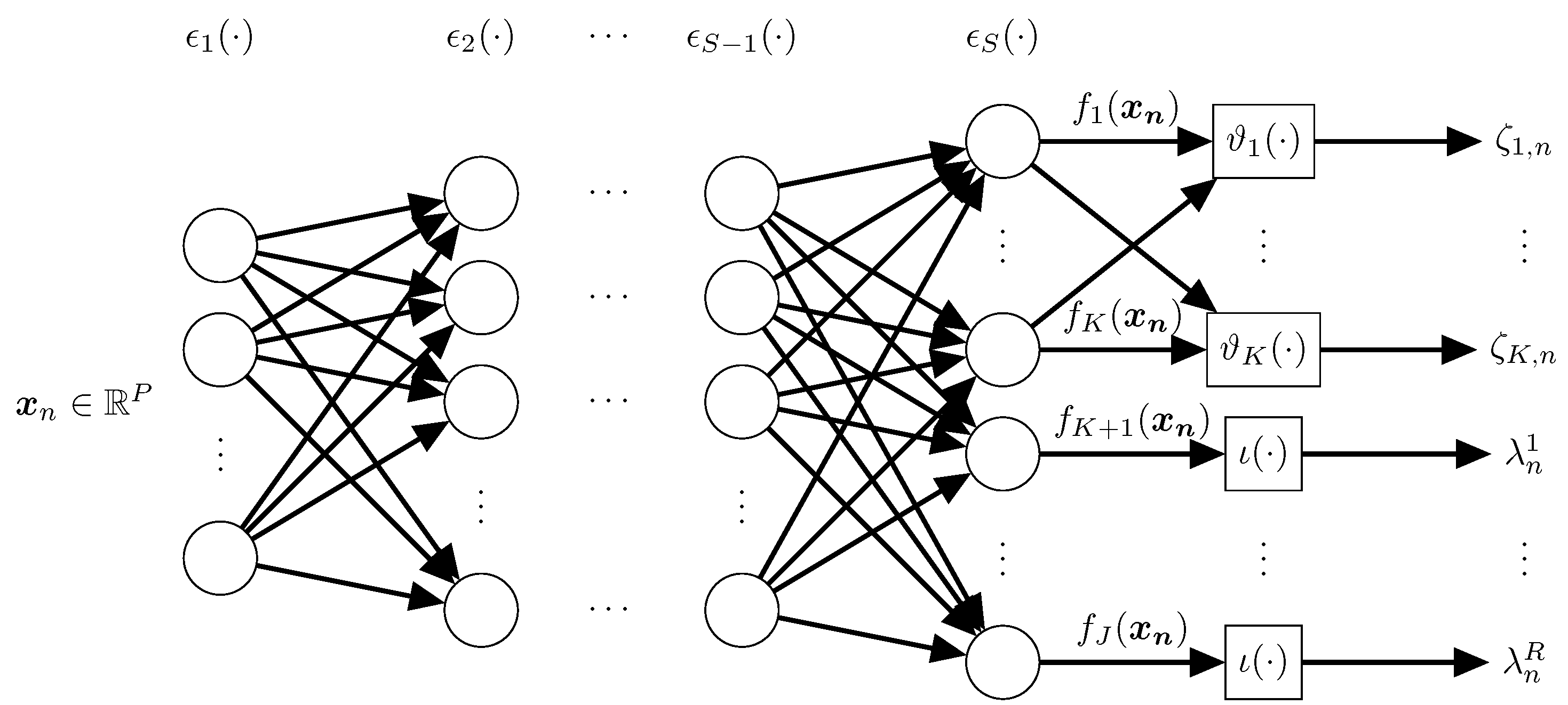
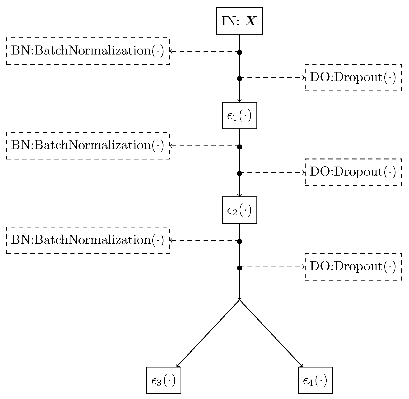
This paper introduces a regularized chained deep neural network for multiple annotators, termed RCDNN, to jointly estimate the ground truth label and the annotators’ performance. RCDNN is inspired in the chained Gaussian processes model (CGP) [25], where each parameter in a given likelihood is coded with multiple independent Gaussian processes–(GP) priors (one GP prior per parameter). Unlike CGP, our method considers that the last layer models the parameters of an arbitrary likelihood. Thus, in a multi-labeler scenario, the annotators’ parameters are coded as a function of the input space. Moreover, since each output in a deep model is computed as a linear combination of previous layers’ outputs, our RCDNN can code interdependencies among the annotators. Besides, l1, l2, and Monte-Carlo Dropout-based regularizers are coupled within our method to deal with the over-fitting issue in deep learning models. Achieved results, using both simulated and real-world data, show how our method can deal with classification problems from multi-labelers data.

The agenda is as follows: Section 2 summarizes the related work. Section 3 describes the methods. Section 4 and Section 5 present the experiments and discuss the results. Finally, Section 6 outlines the conclusions and future work.

2. Related Work

As analyzed by the authors in [26], there exists an increasing interest in developing models to deal with multi-labeler data. However, it is possible to identify some problems that are not entirely solved: (i) to code the relationship between the labelers’ performance and the input space, and (ii) to identify annotators’ interdependencies.

In [23], the authors introduced a binary classification algorithm for multiple labelers, where the input data are represented by Gaussian mixture model (GMM)-based clusters. This approach assumes that each annotator exhibits a particular performance concerning a given cluster. Nevertheless, such a model does not consider the information from multiple annotators as an input for the GMM, leading to variations in the labelers’ parameters. In [27], the authors propose a binary classification algorithm employing two distributions to compute the annotators’ achievement as a function of the input space, namely, Gaussian and Bernoulli. The parameters of such distributions are computed via logistic regression optimization. Still, a linear dependence is assumed between the labeler’s expertise and the input space, which may not be appropriate in the presence of non-linear data structures. For example, if we take into account online annotators assessing documents, they may show different labeling accuracies depending on if they are more familiar with some specific topic [28].

On the other hand, the work in [29] uses a multivariate Gaussian distribution to model the annotations, and the experts’ interdependencies are coded in the covariance matrix. Besides, in [16], the authors introduce a binary classification method based on a weighted combination of classifiers. The weights are computed using a centered kernel alignment (CKA)-based loss to measure the similarities among the input features and the labels from multiple annotators. Similarly, the authors in [1] proposed a localized kernel alignment-based method, termed LKAAR, to build a classification approach with multiple annotators. However, unlike the work in [16], LKAAR modifies the CKA-based loss to measure the similarities among each input instance and its corresponding set of labels. Thereby, LKAAR measures the annotators’ performance as a function of the input space while considering interdependencies among the experts.

Our proposal follows the line of the works in [19,20] in the sense that RCDNN uses a deep-based approach to build a supervised learning model in the context of multiple annotators. However, while such approaches code the annotators’ parameters as fixed points, we model them as functions to consider dependencies between the input features and the labelers’ behavior. RCDNN is also similar to the LKAAR model introduced in [1]. Both approaches model the annotators’ performance as a function of the input instances and consider interdependencies among the labelers. Nonetheless, unlike LKAAR, where it is necessary to use as many classifiers as annotators, our approach only needs to train a single classifier from a deep learning representation, which is advantageous for a large number of labelers. As an illustrative summary,

Table 1. Survey of relevant supervised learning approaches devoted to multiple annotators.

Source	Data Type/Application	Perspective	Expertise as a Function of the Input Space	Modeling the Annotators’ Interdependencies
Raykar et al., 2010 [2]	Regression-Binary-Categorical	Frequentist	✗	✗
Zhang and Obradovic, 2011 [23]	Binary	Frequentist	✓	✗
Xiao et al., 2013 [13]	Regression	Frequentist	✓	✗
Yan et al., 2014 [27]	Binary	Frequentist	✓	✗
Wang and Bi, 2016 [28]	Binary	Frequentist	✓	✗
Rodrigues et al., 2017 [30]	Regression-Binary-Categorical	Frequentist	✗	✗
Gil-Gonzalez et al., 2018 [16]	Binary	Frequentist	✗	✓
Hua et al., 2018 [31]	Binary-Categorical	Frequentist	✗	✗
Ruiz et al., 2019 [9]	Binary	Bayesian	✗	✗
Morales- Alvarez et al., 2019 [15]	Binary	Bayesian	✗	✗
Zhu et al., 2019 [29]	Regression	Bayesian	✗	✓
Gil-Gonzalez et al., 2021 [1]	Binary-Categorical	Frequentist	✓	✓
Proposal-(RCDNN)	Binary-Categorical	Frequentist	✓	✓

shows the key insights of our RCDNN and relevant state-of-the-art works.

3. Methods

3.1. Chained Deep Neural Network

Let us consider an input-output dataset $=\{\mathit{X}\in \mathcal{X},\mathbf{y}\in \mathcal{Y}\},$ where $\mathit{X}={\left\{{\mathit{x}}_n\in \mathcal{X}\subseteq {\mathbb{R}}^P\right\}}_{n=1}^N$ and $\mathbf{y}={\left\{y_n\in \mathcal{Y}\right\}}_{n=1}^N$ hold the input and output spaces, respectively, (with N instances and P features). Inspired by the chained Gaussian processes model (CGP) [25], a likelihood function with J parameters is written as:

$$\begin{array}{c}\hfill p\left(\mathit{y}\right|\mathit{X},\mathbf{\theta })=\prod _{n=1}^{N}p\left(y_n\right|{\theta }_1\left({\mathit{x}}_n\right),\cdots ,{\theta }_J\left({\mathit{x}}_n\right)),\end{array}$$

(1)

where $\mathbf{\theta }={\left[{\mathbf{\theta }}_1\cdots ,{\mathbf{\theta }}_J\right]}^{\top }\in {\mathbb{R}}^{NJ}$ is a parameter vector, and ${\mathbf{\theta }}_j={\left[{\theta }_j\left({\mathit{x}}_1\right)\cdots {\theta }_j\left({\mathit{x}}_N\right)\right]}^{\top }\in {\mathbb{R}}^N$. Here, each ${\theta }_j\left(\mathit{x}\right)={\mathcal{M}}_j$ maps an input sample to the parameter space, being ${\mathcal{M}}_j$ the domain for the j-th parameter ($j\in \left\{1,2,\cdots ,J\right\}$). A chained deep neural network (CDNN) can be introduced linking each likelihood parameter ${\theta }_j\left(\mathit{x}\right)$ to one of the J outputs of a deep neural network comprising S hidden layers. Accordingly, let $\mathit{f}\left(\mathit{x}\right)={[f_1\left(\mathit{x}\right),\cdots ,f_J\left(\mathit{x}\right)]}^{\top }\in {\mathbb{R}}^J$ be a vector containing the J outputs of a deep network:

$$\begin{array}{c}\hfill \mathit{f}\left(\mathit{x}\right)=({ϵ}_S\circ {ϵ}_{S-1}\circ \cdots \circ {ϵ}_1)\left(\mathit{x}\right),\end{array}$$

(2)

where ∘ stands for function composition. Then, each parameter is computed as: ${\theta }_j\left(\mathit{x}\right)=h_j\left(f_j\left(\mathit{x}\right)\right)$, where $h_j:\mathbb{R}\to {\mathcal{M}}_j$ is a deterministic function that maps each output $f_j\left(\mathit{x}\right)$ to the appropriate domain ${\mathcal{M}}_j$. Besides, each layer ${ϵ}_s$, with $s\in \left\{1,2,\cdots ,S\right\}$, depends on a set of variables (neural network weights and bias) $\mathbf{\varphi }={[{\mathbf{\varphi }}_1,\cdots ,{\mathbf{\varphi }}_S]}^{\top }$, which can be estimated by minimizing the following log likelihood cost (for i.i.d samples):

$$\begin{array}{c}\hfill -log\left(p\left(\mathit{y}\right|\mathit{X},\mathbf{\theta },\mathbf{\varphi })\right)=-\sum _{n=1}^{N}log\left(p\left(y_n\right|{\theta }_1\left({\mathit{x}}_n\right),\cdots ,{\theta }_J\left({\mathit{x}}_n\right),\mathbf{\varphi })\right).\end{array}$$

(3)

Remarkably, the deep model in Equation (2) allows exploiting the representation learning capability of neural networks within a chained framework through the likelihood in Equation (3).

3.2. Regularized Chained Deep Neural Network for Multiple Annotators

Let $g:\mathcal{X}\to \mathcal{Y}$ be a classification function trained on the input-output set ${\{{\mathit{x}}_n,y_n\}}_{n=1}^N,$ where ${\mathit{x}}_n\in \mathcal{X}\subseteq {\mathbb{R}}^P$ is a $P-$dimensional input feature vector corresponding to the n-th instance with label $y_n\in \mathcal{Y}\subseteq \left\{1,2,\cdots ,K\right\}$, being K the number of classes. $y_n$ is assumed to be the absolute ground truth. However, in many real-world classification problems, instead of the ground truth, multiple labels are provided by $R={\mathbb{Z}}^{+}$ experts with different levels of ability [12], where the r-th expert annotates $|{\Omega }_r|\le N$ instances, being $|{\Omega }_r|$ the cardinality of the set ${\Omega }_r$ containing the indexes of samples labeled by expert r. Further, let ${\Psi }_n$ be the index set of annotators who labeled the n-th instance. Next, it is possible to build a dataset from multiple annotators $\mathcal{D}=\left\{\mathit{X},\mathbf{Y}={\left\{y_n^r\right\}}_{n=1}^N;r\in {\Psi }_n\right\}$, where $y_n^r$ is the decision of annotator r for instance n.

Following the work proposed by authors in [32]; here, a regularized chained deep neural network (RCDNN) is introduced for classification tasks from multiple annotations. Concerning this, let ${\lambda }_n^r\in \left\{0,1\right\}$ be a binary variable representing the r-th annotator reliability: ${\lambda }_n^r=1$ if $y_n^r=y_n$, and ${\lambda }_n^r=0$ in other case. If ${\lambda }_n^r=1$, the label $y_n^r$ is modeled by means of a categorical distribution; otherwise, if ${\lambda }_n^r=0$, $y_n^r$ is supposed to follow an uniform distribution. In consequence, the likelihood function in Equation (3) is rewritten as:

$$\begin{array}{c}\hfill p\left(\mathit{Y}\right|\mathbf{\theta })=\prod _{n=1}^N\prod _{r\in {\Psi }_n}{\left(\prod _{k=1}^K{\zeta }_{n,k}^{\delta (y_n^r-k)}\right)}^{{\lambda }_n^r}{\left(\frac{1}{K}\right)}^{1-{\lambda }_n^r},\end{array}$$

(4)

where $\delta (y_n^r-k)=1$, if $y_n^r=k$, and $\delta (y_n^r-k)=0$, otherwise. Moreover, ${\zeta }_{n,k}=p(y_n^r=k|{\lambda }_n^r=1)$ is the estimation of the hidden ground truth for the n-th instance in class k.

Accordingly, an architecture holding $J=K+R$ outputs is required within our RCDNN for modeling the likelihood parameters $\mathbf{\theta }$ in Equation (4). In particular, K output layers ${\left\{{\vartheta }_k(·)\right\}}_{k=1}^K$ are fixed to estimate the hidden ground truth ${\zeta }_{n,k}$ based on a softmax function as follows:

$$\begin{array}{c}\hfill {\zeta }_{n,k}={\vartheta }_k(f_1\left({\mathit{x}}_n\right),\cdots ,f_K\left({\mathit{x}}_n\right))=\frac{exp\left(f_k\left({\mathit{x}}_n\right)\right)}{{\sum }_{i=1}^{K}exp\left(f_i\left({\mathit{x}}_n\right)\right)}.\end{array}$$

(5)

Furthermore, a step function can be used to compute the annotator reliability. Yet, the step function is approximated through R output layers ${\left\{{\iota }_r(·)\right\}}_{r=1}^R$, fixing the well-known sigmoid activation to avoid discontinuities and favor the RCDNN implementation:

$$\begin{array}{c}\hfill {\lambda }_n^r=\iota \left(f_m\left({\mathit{x}}_n\right)\right)=\frac{1}{1+exp\left(f_m\left({\mathit{x}}_n\right)\right)},\end{array}$$

(6)

where $m\in \left\{K+1,\cdots J\right\}$ is the index of the output linked to the estimation of the reliability of r-th expert. Afterward, the log likelihood of Equation (4) is used to compute the RCDNN weights and bias in $\mathbf{\varphi }$, as follows:

$$\begin{array}{c}\hfill {\mathbf{\varphi }}^{*}=arg\underset{\mathbf{\varphi }}{min}-\sum _{n=1}^N\sum _{r\in R_n}\left[{\lambda }_n^r\left(\mathbf{\varphi }\right)\left(\sum _{k=1}^K\delta (y_n^r-k)log\left({\zeta }_{n,k}\left(\mathbf{\varphi }\right)\right)\right)-\left(1-{\lambda }_n^r\left(\mathbf{\varphi }\right)\right)log\left(K\right)\right],\end{array}$$

(7)

where ${\lambda }_n^r\left(\mathbf{\varphi }\right)$ and ${\zeta }_{n,k}\left(\mathbf{\varphi }\right)$ highlight the dependency between the annotator reliability/ground truth estimation and the RCDNN weights and bias. Figure 1 summarizes the RCDNN pipeline as a classifier for a dataset holding multiple annotators.

In turn, to avoid over-fitting and favor the RCDNN generalization capability, l1 and l2 norm-based regularizers are used for dense layers; besides, Dropout layers are also added. Of note, both regularization schemes are implemented through the function composition presented in Equation (2). Lastly, to exploit the RCDNN generalization, the well-known Monte-Carlo Dropout prediction strategy is used to estimate the expert’s reliability ${\widehat{\lambda }}_n^r$ and the ground truth label ${\widehat{\zeta }}_{n,k}$, as follows [33]:

$$\begin{array}{cc}\hfill {\widehat{\lambda }}_n^r=& \frac{1}{D}\sum _{d=1}^D{\lambda }_n^r\left({\mathbf{\varphi }}^{*},{\Delta }_d\right),\hfill \end{array}$$

(8)

$$\begin{array}{cc}\hfill {\widehat{\zeta }}_{n,k}^r=& \frac{1}{D}\sum _{d=1}^D{\zeta }_{n,k}^r\left({\mathbf{\varphi }}^{*},{\Delta }_d\right);\hfill \end{array}$$

(9)

where notation ${\lambda }_n^r\left({\mathbf{\varphi }}^{*},{\Delta }_d\right)$ and ${\zeta }_{n,k}^r\left({\mathbf{\varphi }}^{*},{\Delta }_d\right)$ stands for the dependency between the estimated output, the trained RCDNN weights and bias based on Equation (7), and the set ${\Delta }_d$ holding Dropout layers. As seen, the Monte-Carlo Dropout-based predictions in Equations (8) and (9) compute the RCDNN outputs as the sample mean over a stack of D predictions; each of them activates randomly the Dropout layers in ${\Delta }_d$ for the d-th iteration within a Monte-Carlo scheme. For RCDNN’s implementation details see Section 4.4.

4. Experimental Set-Up

4.1. Tested Datasets

The introduced RCDNN classifier for multiple annotators scenarios is tested in three different kind of datasets. The first category, termed 2D-PCA iris dataset, is intended to show graphically how our method works. The principal component analysis (PCA) algorithm is applied to reduce the well-known Iris dataset dimension from four to two [33], aiming to easily observe some preliminary results in a cartesian plane and illustrate how multiple annotations can be simulated.

The second category comprises datasets where the input data come from real-world applications. Still, the labels from multiple annotators are obtained synthetically (Semi-synthetic datasets). The latter is carried out to control the labeling process. In particular, nine datasets of binary and multi-class-classification tasks are studied from the well-known UCI repository. (http://archive.ics.uci.edu/ml, (accessed on 19 April 2021)) The chosen datasets include: Wisconsin Breast Cancer database–(breast); BUPA liver disorders–(bupa); Johns Hopkins University Ionosphere database–(ionosphere); Pima Indians Diabetes database–(pima); Tic-Tac-Toe Endgame database–(tic-tac-toe); Iris Plants database–(iris); Wine data set–(wine); and Image Segmentation dataset–-(segmentation). Besides, the publicly available bearing data collected by the Case Western Reserve University–(Western) is tested. The aim is to build a system to diagnose an electric motor’s status based on two accelerometers. The feature extraction was performed as in [34].

The third category includes Real-world datasets, where both the input features and the labels come from real-world applications. The Massachusetts Eye and Ear Infirmary Disordered Voice Database from the Kay Elemetrics company is proved. A subset holding $N=218$ voice records is considered from both healthy and different voice issues. Each voice record is parametrized using the Mel-frequency cepstral coefficients (MFCC) to obtain an input space with a dimensionality of $P=13$. A set of physicians label each voice record by assessing its quality through the GRBAS protocol, comprising the evaluation of five qualitative scales: Grade of dysphonia (G); Roughness (R); Breathiness (B); Aesthenia (A); and Strain (S). For each scale, the specialist provides a tag ranging from 0 (healthy voice) to 3 (severe disease) [35]. A five multi-class task is built (one per each qualitative scale). However, five binary classification problems are provided to access the ground truth, which is useful for validation purposes [36]. The second dataset is named music genre, which corresponds to a collection of song records with 30 s of length and labeled from one to ten, depending on their music genre: classical, country, disco, hip-hop, jazz, rock, blues, reggae, pop, and metal. A total of 700 samples are selected randomly and published in the AMT platform to obtain labels from multiples sources. The feature extraction is performed by following the work in [32], to obtain an input space with $P=124$ features. The third one is a sentiment polarity dataset, which corresponds to a collection of more than 10,000 sentences labeled as positive or negative. The AMT platform published 4999 sentences to gather answers about their polarity. From this process, 27,747 answers were obtained from 203 labelers. The remaining were kept for testing purposes. Each sample is parametrized following the procedure in [32] to get an input space in $P=1200$ dimensions.

Table 2. A brief description of the tested datasets for synthetic, semi-synthetic, and real-world scenarios.

	Name	Number of	Number of	Number of
		Features (P)	Instances (N)	Classes (K)
synthetic	2D-PCA Iris	2	150	3
semi-synthetic	Breast	9	683	2
	Bupa	6	345	2
	Ionosphere	34	351	2
	Pima	8	768	2
	Tic-tac-toe	9	958	2
	Iris	4	150	3
	Wine	13	178	3
	Segmentation	18	2310	7
	Western	7	3413	4
real-world	Voice	13	218	2
	Music	124	1000	10
	Polarity	1200	10,306	2

summarizes the tested semi-synthetic and real-world datasets.

4.2. Provided and Simulated Annotations

Since the semi-synthetic datasets do not provide annotations from multiple labelers, to test our RCDNN classifier, it is necessary to simulate those annotations based on the ground truth, which is available for this kind of experiments. Considering that our approach models the annotators’ performance as a function of the input space, we simulate labels using two schemes. The former, termed Non-homogeneous labels, represents the input space by R clusters (for concrete testing, we use the K-means algorithm to define each cluster) [27,37]. Then, the r-th annotator is considered an “expert”, i.e., his or her labels correspond to the ground truth in samples belonging to the cluster r. For the rest of the samples, the annotator makes mistakes in the $35\%$ of the cases selected randomly. Similarly, Biased coin (Non-homogeneous) assumes that the input space can be represented by using R clusters [1,32]. In each cluster $c\in \{1,\cdots ,R\}$, a random number ${\alpha }_{n\sim c}^r$ is sampled from a Bernoulli distribution with parameter $p_c^r\in [0,1]$ ($n\sim c$ stands for the instance n belonging to the cluster c). So, the performance of the r-th annotator is modeled in each region c. Then, the simulated annotations of the r-th expert yields: $y_n^r=y_n$, if ${\alpha }_{n\sim c}^r=0$, otherwise, $y_n^r={\tilde{y}}_n$, if ${\alpha }_{n\sim c}^r=1$.

Regarding the voice quality dataset, the annotations from four experts are provided, $R=4$. However, for concrete testing, only the G, R, and B scales are studied. Indeed, for scales A and S, the sources’ expertise are not satisfactory [36]. Similarly, for the polarity sentiment dataset, labels from 203 workers are available. Annotators who labeled at least 15% of the available instances are kept, yielding $R=7$ labelers. Finally, concerning the music dataset, 2946 labels were obtained from 44 instances. Nevertheless, in our experiments, the sources that labeled at least the $15\%$ of the available instances are studied ($R=9$).

4.3. Method Comparison and Quality Assessment

Our model’s validation is carried out by estimating the classification performance as the area under the curve (AUC) and the overall accuracy (Acc). The AUC is extended for multi-class scenarios, as discussed in [38]. A cross-validation scheme is used with 30 repetitions, where 70% of the samples are utilized for training and the remaining $30\%$ for testing, except for the music and polarity dataset since they clearly define the training and testing sets.

Table 3. A short overview of the tested state-of-the-art approaches. GPC: Gaussian processes classifier, LRC: logistic regression classifier, MV: majority voting, MA: multiple annotators, MAE: Modelling annotators expertise, LFC: Learning from crowds, DGRL: distinguishing good from random labelers, KAAR: kernel alignment-based annotator relevance analysis, LKAAR: localized kernel alignment-based annotator relevance analysis.

Approach	Brief Description
GPC-GOLD	A GPC using the real labels (upper bound).
GPC-MV	A GPC using the majority voting of the labels as the ground truth.
MA-LFC [2]	A LRC with constant parameters across the input space.
MA-DGRL [32]	A multi-labeler approach that considers as latent variables the annotator performance.
MA-MAE [37]	A LRC where the sources parameters depend on the input space.
MA-GPC [14]	A multi-labeler GPC, which is an extension of MA-LFC by using a non-linear approach.
KAAR [16]	A kernel-based approach that employs a convex combination of GPC, it codes the labelers dependencies.
LKAAR-(LR,SVM,GPC) [16]	A localized kernel alignment-based annotator relevance analysis using a combination of LRC, SVM, GPC respectively. It models both the annotators dependencies and the relationship between the labelers’ behavior and the input features.

displays the state-of-the-art models that are considered for comparison purposes. The Matlab codes for the state-of-the-art methods studied are publicly available (GPC-MV MA-LFC, MA-MAE, MA-DGRL, GPC-GTIC, KAAR, and LKAAR codes: https://github.com/juliangilg (accessed on 19 April 2021). MA-GPC codes: http://www.fprodrigues.com/ (accessed on 19 April 2021)). Of note, the GPC-Gold is used only to provide an upper bound for our approach.

4.4. RCDNN Detailed Architecture and Training

The proposed RCDNN architecture for multiple annotators comprises:

–

IN: An input layer fed by the input samples $\mathit{X}\in {\mathbb{R}}^{N\times P}$;

–

${ϵ}_1(·)$: A dense layer coding relevant patterns from input features to perform. The number of neurons is set as $h=\lfloor \rho P\rceil$, where $\rho \in \{0.5,1,1.5\}$ is chosen empirically; a linear-based activation function is used to code input data linear dependencies;

–

${ϵ}_2(·)$: A dense layer fixing a tanh-based activation function with $J=K+R$ neurons to reveal non-linear relationships;

–

${ϵ}_3(·)$: A fully-connected layer with K neurons and a softmax-based activation function, which is employed to estimate the hidden ground truth ${\zeta }_{k,n}$;

–

${ϵ}_4(·)$: A dense layer with R neurons and a sigmoid-based activation function, which is used to compute the annotators’ reliability in ${\lambda }_n^r$;

–

For all provided ${ϵ}_s$ layers l1 plus l2-based regularization strategy is used, searching the regularization weights within the range {1e-3,1e-2,1e-1};

–

Batch Normalization and Dropout layers are included between layers to avoid vanishing and exploding gradient issues. Additionally, it favors the RCDNN’s generalization capability as exposed in Section 3.2. See Figure 2 for details;

–

The optimization problem in Equation (7) is solved by using a Back-propagation algorithm as usual. Moreover, to favor scalability, we utilize a mini-batch-based gradient descent approach with automatic differentiation (RMSprop-based optimizer is fixed).

We clarify that our RCDNN is flexible, and it admits different deep structures such as recurrent or convolutional layers aiming to deal with complex tasks (e.g., computer vision or natural language processing). Moreover, our approach can build from different activation functions (RELU, ELU, sigmoid, softmax). However, the last layers (in this particular case ${ϵ}_3$ and ${ϵ}_4$) need to be designed to code each annotator’s behavior and the hidden ground truth. For example, the parameter ${\lambda }_n^r$ represents an estimation for the annotators’ reliability; accordingly, we need to use an activation function whose output belongs to the range $[0,1]$.

5. Results and Discussion

5.1. Synthetic Dataset Results

A controlled experiment is performed to estimate the performance of inconsistent labelers as a function of the input space while highlighting their dependencies. For this first experiment, the 2D PCA Iris dataset is employed (see Section 4.1). Besides, the data are divided into five clusters using the K-means technique to emulate five annotators using the approach “Biased coin (Non-homogeneous)”. A matrix $\mathit{A}\in {[0,1]}^{R\times R}$ is used to set a different score (annotator reliability) for each pair annotator-cluster, as follows:

$$\begin{array}{c}\hfill \mathit{A}=\left(\begin{array}{ccccc}0& 0.9& 0.5& 0.15& 0.6\\ 0.9& 0& 0.3& 0.4& 0.75\\ 0.5& 0.3& 0& 0.6& 0.3\\ 0.15& 0.4& 0.6& 0& 0.8\\ 0.6& 0.75& 0.3& 0.8& 0\end{array}\right).\end{array}$$

(10)

Note that the value $a_{c,r}$ refers to the probability that the annotator r fails labeling a sample that belongs to the cluster c; thus, a zero-value means a perfect annotator for the correspondent cluster. The r-th annotator is an expert (its labels correspond to the ground truth) in the region $c=r$.

Figure 3 shows the decision boundaries generated by our approach for the first experiment. As shown, RCDNN offers a suitable representation for the multi-class classification problem; an AUC score of $0.9837$ is achieved, which demonstrates its generalization capability, even in cases where the ground truth is unknown. Indeed, RCDNN codes both the relationship between the input space and the annotator’s behavior and the dependencies among their labels, which improves the quality of the expert codification [1,16,29]. To empirically support the above statement, Figure 4 shows each annotator’s simulated accuracy and the reliability estimated by our RCDNN. The latter elucidates how our method performs a satisfactory identification of the zones where the labelers have the best accuracy. The above is not unexpected because the annotators’ accuracy (simulated) is compared with their reliability (estimated); hence, the regions where a specific labeler obtains the higher accuracy should match the regions where the estimated reliability is closer to 1.

In addition, Figure 5 shows a comparison between the Pearson correlation coefficients (absolute value) from the labelers’ performance in Equation (10), configuring the simulated dependencies among the annotators, and the Pearson correlation coefficients (absolute value) from the weight matrix ${\Phi }_{{ϵ}_4}\in {\mathbb{R}}^{(K+R)\times R}$ of the layer ${ϵ}_4(·)$ (RCDNN annotators’ dependencies estimation). Comparing the real and the estimated dependencies, it is noticeable that, even though the exact matrix is not recovered, our approach efficiently finds tendencies between annotators’ performances. Thereby, the learned representation from hidden layers (see Figure 2) allows coding both linear and non-linear patterns that recover the expert dependencies from data. Then, our deep model estimates the unknown ground truth and the relationships between annotators.

5.2. Semi-Synthetic Datasets Results

Table 4. Semi-synthetic datasets results for Non-homogeneous labels. Bold: the highest AUC excluding the upper bound (target) classifier GPC-GOLD. Marked with *: the highest accuracy (Acc) except the upper bound. The last column presents the average ranking for both the AUC score and the overall accuracy (GPC-GOLD is not considered), the best average ranking for AUC is highlighted in bold, and the accuracy is marked with *. From the Friedman test we obtain a Chi-square of $12.21$ (p-value = 0.2).

Method		Breast	Bupa	Ionosphere	Pima	Tic-Tac-Toe	Iris	Wine	Segmentation	Western	Average AUC-Acc	Average Ranking
GPC-GOLD	AUC[%]	$99.04\pm 0.94$	$72.21\pm 3.69$	$95.02\pm 2.44$	$83.76\pm 1.98$	$99.97\pm 0.06$	$97.65\pm 2.71$	$99.22\pm 0.67$	$90.08\pm 1.94$	$94.52\pm 0.57$	$92.39$	-
	Acc[%]	$96.44\pm 1.54$	$68.48\pm 4.43$	$91.08\pm 2.41$	$76.71\pm 1.96$	$99.16\pm 0.85$	$95.85\pm 3.29$	$96.92\pm 1.44$	$70.68\pm 6.81$	$79.75\pm 0.57$	$86.12$	-
GPC-MV	AUC[%]	$99.11\pm 0.58$	$70.95\pm 3.90$	$93.14\pm 3.49$	$81.21\pm 2.57$	$87.83\pm 4.11$	$99.63\pm 0.39$	$98.41\pm 1.38$	$91.48\pm 1.48$	$78.14\pm 4.15$	$88.87$	$5.77$
	Acc[%]	$96.29\pm 1.48$	$66.60\pm 4.31$	$87.90\pm 3.26$	$74.87\pm 2.32$	$81.96\pm 3.46$	$95.33\pm 3.05$	$93.96\pm 3.34$	$82.68\pm 5.30$	$63.35\pm 1.68$	$82.54$	$4.88$
MA-LFC	AUC[%]	$98.72\pm 0.93$	$\mathbf{71}.\mathbf{53}\pm \mathbf{4}.\mathbf{18}$	$82.08\pm 4.79$	$82.29\pm 2.22$	$61.13\pm 3.28$	$98.75\pm 1.44$	$96.83\pm 1.75$	$\mathbf{99}.\mathbf{58}\pm \mathbf{0}.\mathbf{11}$	$87.77\pm 0.79$	$86.72$	$5.33$
	Acc[%]	$95.63\pm 1.79$	$\mathbf{69}.\mathbf{68}\pm \mathbf{4}.\mathbf{20}$ *	$81.43\pm 4.44$	$\mathbf{76}.\mathbf{52}\pm \mathbf{1}.\mathbf{91}$ *	$64.88\pm 2.86$	$94.44\pm 4.62$	$87.74\pm 4.67$	$\mathbf{95}.\mathbf{40}\pm \mathbf{0}.\mathbf{71}$ *	$57.21\pm 1.32$	$80.32$	$6.11$
MA-DGRL	AUC[%]	$99.30\pm 0.39$	$68.00\pm 4.09$	$77.60\pm 7.50$	$81.72\pm 2.57$	$61.83\pm 2.80$	$98.78\pm 1.34$	$95.33\pm 3.35$	$98.31\pm 0.32$	$87.67\pm 0.85$	$85.39$	$6.44$
	Acc[%]	$94.63\pm 1.77$	$65.77\pm 3.47$	$81.94\pm 3.42$	$76.45\pm 2.81$	$66.45\pm 2.24$	$94.59\pm 2.96$	$84.91\pm 6.50$	$89.58\pm 0.99$	$60.55\pm 1.26$	$79.43$	$7.11$
MA-MAE	AUC[%]	$99.28\pm 0.60$	$70.82\pm 3.90$	$78.91\pm 6.01$	$81.80\pm 2.57$	$60.35\pm 3.28$	$85.97\pm 2.39$	$98.20\pm 1.33$	$97.27\pm 0.28$	$72.83\pm 0.80$	$82.76$	$7.33$
	Acc[%]	$96.31\pm 1.38$	$66.92\pm 3.35$	$82.25\pm 3.99$	$76.12\pm 2.77$	$65.64\pm 2.37$	$94.81\pm 4.14$	$89.31\pm 5.79$	$92.94\pm 0.76$	$52.41\pm 1.56$	$79.63$	$5.77$
MA-GPC	AUC[%]	$95.81\pm 2.94$	$49.81\pm 11.72$	$94.46\pm 3.09$	$67.83\pm 4.24$	$81.44\pm 3.81$	$99.15\pm 1.03$	$99.85\pm 0.24$	$99.42\pm 0.14$	$\mathbf{94}.\mathbf{14}\pm \mathbf{0}.\mathbf{52}$	$86.87$	$5.22$
	Acc[%]	$96.70\pm 1.37$ *	$59.52\pm 4.71$	$82.13\pm 3.32$	$72.77\pm 2.71$	$76.39\pm 2.85$	$94.30\pm 2.90$	$94.34\pm 2.80$	$94.74\pm 0.68$	$\mathbf{78}.\mathbf{52}\pm \mathbf{1}.\mathbf{11}$ *	$\mathbf{83}.\mathbf{26}$ *	$5.55$
KAAR	AUC[%]	$98.81\pm 0.66$	$70.20\pm 5.70$	$93.88\pm 3.53$	$81.18\pm 2.93$	$89.55\pm 2.84$	$99.56\pm 0.52$	$99.53\pm 0.36$	$92.34\pm 1.38$	$81.77\pm 1.02$	$89.64$	$5.55$
	Acc[%]	$96.02\pm 1.14$	$65.99\pm 5.44$	$87.52\pm 4.24$	$75.10\pm 2.98$	$81.68\pm 2.41$	$\mathbf{95}.\mathbf{56}\pm \mathbf{2}.\mathbf{92}$ *	$96.54\pm 2.11$	$81.11\pm 4.15$	$64.58\pm 1.47$	$82.67$	$4.77$
LKAAR-LR	AUC[%]	$99.34\pm 0.44$	$68.86\pm 5.16$	$87.14\pm 3.38$	$82.04\pm 2.44$	$65.40\pm 3.13$	$96.00\pm 2.50$	$99.21\pm 0.82$	$97.97\pm 0.27$	$83.25\pm 1.22$	$86.57$	$5.66$
	Acc[%]	$96.00\pm 1.46$	$64.17\pm 4.22$	$84.10\pm 3.20$	$75.67\pm 2.15$	$66.96\pm 2.74$	$82.59\pm 6.07$	$94.28\pm 3.19$	$90.02\pm 0.93$	$51.49\pm 2.05$	$78.36$	$7.22$
LKAAR-SVM	AUC[%]	$98.29\pm 0.80$	$64.37\pm 3.36$	$\mathbf{96}.\mathbf{98}\pm \mathbf{2}.\mathbf{01}$	$77.80\pm 2.28$	$89.82\pm 2.14$	$98.05\pm 1.90$	$99.53\pm 0.47$	$97.89\pm 0.32$	$79.08\pm 0.95$	$89.09$	$6.33$
	Acc[%]	$96.36\pm 1.02$	$63.14\pm 3.67$	$\mathbf{92}.\mathbf{19}\pm \mathbf{2}.\mathbf{43}$ *	$72.52\pm 2.22$	$80.99\pm 2.81$	$84.44\pm 6.76$	$96.48\pm 2.26$	$91.28\pm 0.93$	$53.73\pm 2.06$	$81.79$	$5.88$
LKAAR-GPC	AUC[%]	$99.00\pm 0.75$	$71.07\pm 5.05$	$93.37\pm 2.91$	$81.23\pm 2.21$	$\mathbf{91}.\mathbf{97}\pm \mathbf{2}.\mathbf{01}$	$99.57\pm 0.61$	$99.64\pm 0.34$	$92.61\pm 1.73$	$81.37\pm 1.37$	$\mathbf{89}.\mathbf{98}$	$4.44$
	Acc[%]	$96.03\pm 1.32$	$66.92\pm 4.79$	$87.75\pm 3.90$	$75.10\pm 2.65$	$\mathbf{84}.\mathbf{09}\pm \mathbf{2}.\mathbf{43}$ *	$95.26\pm 3.29$	$96.54\pm 2.16$	$80.98\pm 3.91$	$65.20\pm 1.72$	$82.65$	$4.44$
RCDNN (ours)	AUC[%]	$\mathbf{99}.\mathbf{47}\pm \mathbf{0}.\mathbf{33}$	$69.80\pm 6.07$	$92.60\pm 2.80$	$\mathbf{83}.\mathbf{25}\pm \mathbf{3}.\mathbf{13}$	$71.17\pm 3.76$	$\mathbf{99}.\mathbf{74}\pm \mathbf{0}.\mathbf{26}$	$\mathbf{99}.\mathbf{90}\pm \mathbf{0}.\mathbf{13}$	$99.15\pm 0.19$	$89.61\pm 0.71$	$89.41$	$\mathbf{3}.\mathbf{00}$
	Acc[%]	$\mathbf{97}.\mathbf{06}\pm \mathbf{1}.\mathbf{19}$ *	$63.69\pm 4.26$	$86.79\pm 2.37$	$76.00\pm 3.10$	$68.06\pm 3.02$	$95.33\pm 2.46$	$\mathbf{97}.\mathbf{84}\pm \mathbf{1}.\mathbf{86}$ *	$92.96\pm 1.06$	$66.46\pm 1.82$	$82.68$	$\mathbf{3}.\mathbf{66}$ *

shows the results concerning the “Non-homogeneous labels”, where it is supposed that the labelers’ performance depends on the input space $\mathcal{X}$. We show the non-parametric Friedman test results to establish their statistical significance. The null hypothesis settles that all algorithms perform equal [39]. Additionally, we fix the significance threshold as $p<0.05$. The GPC-GOLD standard is not included within the test to compare only multiple annotators approaches. First, we notice that most of the classification schemes present a considerably high performance for both AUC and Acc; in fact, the average AUC and Acc for all methods (except MA-DGRL and MA-MAE) are similar compared to the upper bound GPC-GOLD. The above behavior demonstrates high-quality labels, which is confirmed considering the performance of the most naive approach GPC-MV. Furthermore, we highlight that our RCDNN presents the best average ranking and the second AUC and Acc scores. Then, from non-linear-based approaches, we notice that a naive approach, as GPC-MV, obtains similar performance compared with sophisticated ones, such as KAAR, LKAAR-SVM, and LKAAR-GPC. Nevertheless, as we already comment, such an outcome is a consequence of simulating annotators with suitable quality, which favors the majority voting method. Besides, MA-GPC presents the lowest average ranking compared with its other non-linear methods, resulting from a lack of generalization (over-fitting). Regarding the results for the linear models, they achieve lower performance than non-linear ones. As seen, there is no statistical evidence to establish that our RCDNN outperforms its competitors (p-value = 0.2). We explain such an outcome because, for this experiment, the quality of the labels is significantly high; thus, similar performances are obtained.

On the other hand,

Table 5. Semi-synthetic datasets results for Biased coin (Non-homogeneous) labels. Bold: the highest AUC excluding the upper bound (target) classifier GPC-GOLD. Marked with *: the highest accuracy (Acc) except the upper bound. The last column presents the average ranking for both the AUC score and the overall accuracy (GPC-GOLD is not considered), the best average ranking for AUC is highlighted in bold, and the accuracy is marked with *. The Friedman test returns a Chi-square value of $21.16$ (p-value = 0.01).

Method		Breast	Bupa	Ionosphere	Pima	Tic-Tac-Toe	Iris	Wine	Segmentation	Western	Average AUC-Acc	Average Ranking
GPC-GOLD	AUC[%]	$99.04\pm 0.94$	$72.21\pm 3.69$	$95.02\pm 2.44$	$83.76\pm 1.98$	$99.97\pm 0.06$	$97.65\pm 2.71$	$99.22\pm 0.67$	$90.08\pm 1.94$	$94.52\pm 0.57$	$92.39$	-
	Acc[%]	$96.44\pm 1.54$	$68.48\pm 4.43$	$91.08\pm 2.41$	$76.71\pm 1.96$	$99.16\pm 0.85$	$95.85\pm 3.29$	$96.92\pm 1.44$	$70.68\pm 6.81$	$79.75\pm 1.28$	$86.12$	-
GPC-MV	AUC[%]	$90.78\pm 4.28$	$50.47\pm 6.19$	$82.91\pm 6.03$	$70.18\pm 6.29$	$65.91\pm 6.72$	$98.55\pm 1.38$	$97.75\pm 2.04$	$90.18\pm 1.71$	$74.40\pm 4.94$	$80.13$	$7.44$
	Acc[%]	$86.63\pm 2.06$	$48.27\pm 4.84$	$75.65\pm 6.45$	$66.52\pm 5.16$	$64.66\pm 3.64$	$88.81\pm 5.00$	$86.92\pm 5.76$	$79.24\pm 4.99$	$65.04\pm 1.52$	$73.53$	$6.77$
MA-LFC	AUC[%]	$97.99\pm 0.99$	$59.64\pm 8.08$	$72.66\pm 9.98$	$72.73\pm 3.43$	$52.88\pm 3.13$	$96.72\pm 8.98$	$96.47\pm 2.13$	$\mathbf{99}.\mathbf{50}\pm \mathbf{0}.\mathbf{15}$	$84.97\pm 0.84$	$81.51$	6.22
	Acc[%]	$\mathbf{96}.\mathbf{00}\pm \mathbf{1}.\mathbf{70}$ *	$56.41\pm 8.12$	$69.17\pm 12.53$	$58.10\pm 4.53$	$46.27\pm 3.03$	$92.30\pm 5.18$	$87.55\pm 4.97$	$\mathbf{95}.\mathbf{06}\pm \mathbf{0}.\mathbf{80}*$	$55.17\pm 1.33$	$72.89$	6.11
MA-DGRL	AUC[%]	$99.31\pm 0.42$	$61.77\pm 6.17$	$77.83\pm 7.02$	$81.66\pm 2.65$	$55.70\pm 3.95$	$98.76\pm 1.33$	$95.26\pm 3.30$	$98.32\pm 0.34$	$86.61\pm 1.10$	$83.91$	$4.66$
	Acc[%]	$78.08\pm 2.22$	$55.64\pm 4.52$	$71.43\pm 5.15$	$\mathbf{76}.\mathbf{90}\pm \mathbf{1}.\mathbf{99}$ *	$60.64\pm 2.33$	$94.37\pm 2.66$	$84.84\pm 6.32$	$89.63\pm 0.89$	$65.61\pm 1.28$	$75.24$	$5.55$
MA-MAE	AUC[%]	$95.22\pm 1.70$	$64.63\pm 9.77$	$64.18\pm 9.17$	$79.94\pm 2.64$	$52.36\pm 4.78$	$93.16\pm 5.08$	$96.25\pm 2.40$	$94.40\pm 1.26$	$61.40\pm 0.93$	$77.95$	$7.66$
	Acc[%]	$87.15\pm 1.85$	$62.34\pm 8.46$	$67.94\pm 7.19$	$75.94\pm 2.69$	$53.33\pm 6.42$	$81.70\pm 11.68$	$86.67\pm 5.15$	$88.38\pm 2.00$	$49.34\pm 4.15$	$72.53$	$7.00$
MA-GPC	AUC[%]	$85.37\pm 5.90$	$40.79\pm 12.30$	$74.52\pm 4.57$	$73.17\pm 3.34$	$61.82\pm 4.51$	$98.71\pm 1.14$	$99.60\pm 0.41$	$99.35\pm 0.14$	$\mathbf{93}.\mathbf{09}\pm \mathbf{0}.\mathbf{58}$	$80.71$	$5.55$
	Acc[%]	$92.55\pm 2.17$	$52.82\pm 6.38$	$69.87\pm 4.41$	$62.42\pm 3.00$	$62.33\pm 2.98$	$93.85\pm 3.49$	$95.09\pm 2.65$	$93.46\pm 0.83$	$\mathbf{76}.\mathbf{88}\pm \mathbf{1}.\mathbf{19}*$	$77.70$	$4.44$
KAAR	AUC[%]	$97.81\pm 0.99$	$56.52\pm 9.13$	$82.20\pm 4.93$	$67.90\pm 3.16$	$75.34\pm 4.70$	$98.75\pm 1.10$	$97.91\pm 1.36$	$91.75\pm 1.41$	$82.30\pm 0.73$	$83.39$	$6.22$
	Acc[%]	$77.19\pm 3.14$	$52.44\pm 7.79$	$72.60\pm 4.80$	$61.20\pm 2.95$	$70.69\pm 3.63$	$90.44\pm 5.48$	$91.45\pm 4.28$	$76.38\pm 5.05$	$64.61\pm 1.36$	$73.00$	$6.88$
LKAAR-LR	AUC[%]	$\mathbf{99}.\mathbf{52}\pm \mathbf{0}.\mathbf{30}$	$\mathbf{66}.\mathbf{07}\pm \mathbf{6}.\mathbf{14}$	$82.99\pm 5.01$	$80.57\pm 3.31$	$52.32\pm 3.38$	$96.83\pm 2.14$	$99.27\pm 0.68$	$97.87\pm 0.30$	$81.03\pm 0.80$	$84.05$	$4.55$
	Acc[%]	$92.47\pm 2.24$	$\mathbf{60}.\mathbf{22}\pm \mathbf{5}.\mathbf{67}$ *	$78.92\pm 4.32$	$75.07\pm 2.65$	$55.64\pm 2.77$	$83.41\pm 6.92$	$94.59\pm 3.12$	$89.77\pm 0.99$	$54.80\pm 2.05$	$76.10$	$4.88$
LKAAR-SVM	AUC[%]	$98.37\pm 1.00$	$52.35\pm 6.40$	$\mathbf{88}.\mathbf{28}\pm \mathbf{5}.\mathbf{13}$	$66.84\pm 3.66$	$73.85\pm 3.43$	$96.22\pm 2.50$	$98.88\pm 0.80$	$97.59\pm 0.34$	$79.19\pm 1.46$	$82.39$	$5.88$
	Acc[%]	$87.72\pm 5.17$	$50.96\pm 6.81$	$\mathbf{84}.\mathbf{73}\pm \mathbf{4}.\mathbf{66}$ *	$64.81\pm 3.11$	$70.02\pm 2.74$	$74.15\pm 7.90$	$91.82\pm 4.33$	$90.37\pm 1.24$	$55.39\pm 3.03$	$74.44$	$5.66$
LKAAR-GPC	AUC[%]	$98.14\pm 1.04$	$58.36\pm 7.24$	$86.23\pm 4.47$	$73.80\pm 2.83$	$\mathbf{80}.\mathbf{02}\pm \mathbf{4}.\mathbf{15}$	$\mathbf{99}.\mathbf{61}\pm \mathbf{0}.\mathbf{61}$	$98.74\pm 0.93$	$92.24\pm 1.80$	$83.35\pm 0.75$	$85.61$	$4.22$
	Acc[%]	$86.76\pm 4.33$	$54.52\pm 5.27$	$78.25\pm 5.51$	$69.64\pm 3.01$	$\mathbf{74}.\mathbf{90}\pm \mathbf{2}.\mathbf{99}$ *	$\mathbf{95}.\mathbf{93}\pm \mathbf{3}.\mathbf{15}$ *	$93.84\pm 3.57$	$78.71\pm 4.18$	$66.58\pm 1.19$	$77.68$	$4.22$
RCDNN (ours)	AUC[%]	$99.26\pm 0.42$	$64.16\pm 3.87$	$83.41\pm 6.28$	$\mathbf{82}.\mathbf{08}\pm \mathbf{3}.\mathbf{27}$	$65.31\pm 3.87$	$99.51\pm 0.53$	$\mathbf{99}.\mathbf{77}\pm \mathbf{0}.\mathbf{22}$	$99.06\pm 0.20$	$87.94\pm 1.03$	$\mathbf{86}.\mathbf{72}$	$\mathbf{2}.\mathbf{55}$
	Acc[%]	$94.07\pm 2.00$	$58.24\pm 5.13$	$76.70\pm 6.19$	$74.91\pm 3.77$	$65.07\pm 1.17$	$93.33\pm 3.30$	$\mathbf{96}.\mathbf{17}\pm \mathbf{2}.\mathbf{57}$ *	$91.28\pm 0.99$	$61.56\pm 5.13$	$\mathbf{79}.\mathbf{04}$ *	$\mathbf{3}.\mathbf{44}$

shows the results concerning the simulation method “Biased coin (Non-homogeneous)”. At first sight, there exists a generalized lower performance compared with previous results in Table 4. To explain such an outcome, we recall the stimulation parameters $\mathit{A}$ in Equation (10), where the element $1-a_{c,r}$ (column r, row c) indicates the r-th annotator’s performance in region c. Accordingly, taking the average by column to the matrix $1-\mathit{A}$, we obtain the annotators accuracy $[0.57,0.53,0.66,0.61,0.51]$. We remark that the labelers’ accuracy is considerably low for this experiment, which impacts the algorithms’ performance. RCDNN achieves the best predictive performance in both the overall accuracy and the AUC score; RCDNN also obtains the best average ranking. Moreover, the non-linear competitors KAAR, LKAAR-GPC, and LKAAR-SVM achieve competitive results. However, GPC-MV and MA-GPC offer the lowest classification scores. Regarding GPC-MV, the result is explained because GPC-MV corresponds to the most naive approach. After all, it considers that the whole annotators achieve similar performance. On the other hand, the MA-GPC achieves a similar performance compared with GPC-MV; such a behavior proves that MA-GPC is more prone to over-fitting [9]. Remarkably, simple classifiers as MA-LFC, MA-DGRL, and LKAAR-LR obtain competitive outcomes compared to the non-linear competitors; in fact, all the linear models excepting MA-MAE outperform GPC-MV and MA-GPC. An additional experiment is conducted: An LR-based classifier using the ground truth (following a similar scheme for GPC-GOLD) is trained overall datasets, obtaining an average AUC equal to $87.21$ (close enough to the MA-DGRL and LKAAR-LR performances). Accordingly, a linear structure is presented in some of the studied datasets. In turn, MA-MAE obtains the worst generalization performance (even worse than GPC-MV). Such an outcome is a consequence of over-fitting, empirically demonstrated in [16]. Of note, RCDNN and LKAAR-GP obtain similar results, which is expected since both approaches compute the annotators’ performance as a function of the input space while taking into account dependencies between the labelers. However, an unexpected result regarding the “tic-tac-toe” dataset arises, where LKAAR-GP far exceeds the performance of our approach. The above outcome is caused by the categorical features in such a dataset, which cannot be modeled with the chosen DNN architecture Figure 2. Still, our method can be easily adapted by setting different layers and activation functions. Likewise, we apply the Friedman test to verify the significance of results in Table 5. As seen, we obtain a Chi-square of $21.16$ with p-value = 0.01. Thus, we have enough statistical evidence to determine that our approach exhibits the best performance than state-of-the-art competitors.

It is worth noting that the previous experiments were done under controlled scenarios using simulated annotations aiming to stress our method and compare its performance with recently developed approaches. In short, RCDNN offers the best advantages among the state-of-the-art models considered in AUC, overall accuracy, and average ranking.

5.3. Real-World Datasets Results

Up to this point, RCDNN unravels the information hidden in noisy annotations (simulated) to estimate the unknown ground truth considering experts’ performance as a function of the input space and dependencies among labelers. However, the following experiments aim to demonstrate how our approach can outperform state-of-the-art methods even for real labelers, e.g., the challenge is higher as the input data and the annotations are obtained from real-world applications.

Table 6. Fully real-world datasets results. Bold: the method with the highest performance excluding the upper bound (target) classifier GPC-GOLD. The last column presents the average ranking for AUC score, in bold the best average ranking. The Friedman test returns a Chi-square value of $26.71$ (p-value = 0.0015).

AUC([%])
Method	Voice Dataset			Polarity Dataset	Music	Average AUC	Average Ranking
	G	R	B
GPC-GOLD	$93.66$	$93.66$	$93.66$	$80.26$	$92.84$	$90.81$	-
GPC-MV	$90.17$	$84.73$	$84.04$	$71.14$	$88.79$	$83.77$	$6.8$
MA-LFC	$89.99$	$90.59$	$87.27$	$72.06$	$85.99$	$85.18$	$6.4$
MA-DGRL	$85.45$	$90.14$	$79.33$	$56.13$	$88.32$	$79.86$	$8.4$
MA-MAE	$91.08$	$89.12$	$80.74$	$48.73$	$81.92$	$78.31$	$8.4$
MA-GPC	$91.50$	$91.16$	$80.81$	$61.18$	$82.53$	$81.43$	$6.8$
KAAR	$89.85$	$93.50$	$89.20$	$\mathbf{77}.\mathbf{46}$	$88.96$	$87.79$	$3.8$
LKAAR-LR	$90.39$	$92.92$	$88.94$	$68.28$	$84.43$	$84.99$	$6.0$
LKAAR-SVM	$92.06$	$93.02$	$86,98$	$72.70$	$89.98$	$87.70$	$3.6$
LKAAR-GPC	$90.78$	$93.60$	$89.79$	$76.50$	$86.44$	$87.42$	$3.4$
RCDNN (ours)	$\mathbf{92}.\mathbf{24}$	$\mathbf{94}.\mathbf{19}$	$\mathbf{92}.\mathbf{57}$	$76.04$	$\mathbf{93}.\mathbf{29}$	$\mathbf{89}.\mathbf{66}$	$\mathbf{1}.\mathbf{4}$

describes the results achieved using AUC as the metric to compare the state-of-the-art methods in five different real-world datasets.

First, analyzing the voice data, for the scales G and R, all the approaches give similar AUC values. In fact, for the scale G, the GPC-MV attains competitive performance. The latter can be explained in the sense that the annotators exhibit similar conduct for these scales [36]. Conversely, for B scale, a generalized reduction is presented. Looking at RCDNN results for this database, it is noticeable that the achievement is similar among all the scales, which is an exceptional outcome that shows our method’s capabilities to detect regions where annotators have superior execution.

In the polarity dataset, an acceptable RCDNN’s performance is attained compared to others. Our approach requires defining several layer weights in the deep model (Figure 2) concerning the number of features (P), labelers (R), and classes (K). For this particular dataset, those values are considerably higher: $P=1200$, $R=7$, and $K=2$. Nevertheless, the introduced regularization strategy (l1, l2, plus Monte-Carlo Dropout) allows computing an acceptable AUC performance of $76.04$ in comparison with the best achieved by the KAAR method $77.46$.

In the case of music data, our RCDNN obtains the best classification performance. On the other hand, MA-MAE and MA-GPC exhibit a significantly low performance, even lower than the intuitive lower bound (GPC-MV). This behavior has been repeated in the previous experiments because of the over-fitting issue. Nevertheless, an additional challenge is presented for the music dataset regarding the multi-class classification setting. Accordingly, a one-vs-all scheme is fixed for all of the binary classification methods (including MA-MAE and MA-GPC). Such a scheme to deal with multi-class classification can lead regions on the input space that are ambiguously classified [40].

Lastly, like for the semi-synthetic datasets, we perform a Friedman test to validate the significance for the results in Table 6. We obtain a Chi-square value of 26.71 with a significance of p-value = 0.0015; thus, we reject the null hypothesis and conclude that the performance of our approach statistically defeats its competitors.

5.4. Introducing Spammers and Malicious Annotators

As a final experiment, we wish to analyze the impact of spammers and malicious annotators on the performance of our multi-labeler classifier. For concrete testing, we use the pima dataset, which holds 768 instances; from this dataset, we use 538 samples for training and the remaining 230 for testing. We create synthetic labels from 5 annotators generated from the biased coin (Non-homogeneous) procedure (see Section 4.2 and Equation (10)). According to Figure 6 (blue dots), we notice that from the 5 labelers, two are categorized as suitable labelers, one as Spammers and the remaining as Malicious. Then, we add $R_e$ additional annotators aiming to test our approach in extreme scenarios, where the number of malicious or spammers annotators increases. The labels are simulated as follows: A random number ${\alpha }_n^r$ is sampled from a Bernoulli distribution with parameter $p_r$; then if ${\alpha }_n^r=0$, $y_n^r=y_n$, and $y_n^r={\tilde{y}}_n$ otherwise. For Spammers, we use $R_e=65$, and $p_r=0.5$ (see red dots in Figure 6); alike, for malicious labelers, we fix $R_e=20$, and $p_r=0.6$ (see green dots in Figure 6).

Figure 7 presents the classifiers’ performance as a function of the number of spammers (left in Figure 7) and malicious annotators (in right Figure 7). First, we analyze the effect of Spammers annotators on the RCDNN’s performance. From the results in Figure 7 (left), we remark that when the number of Spammers is less than 40, the performance of our approach is not affected. However, when the number of Spammers exceeds 40, the RCDNN’ AUC becomes unstable, oscillating between 0.6 and 0.8. Accordingly, we highlight that the critical point is presented when the percentages of good, spammers and malicious labelers are, respectively, $4.65\%$, $90.70\%$, and $4.65\%$; which shows that our RCDNN is robust in the presence of a high number of Spammers. Now, we compare our RCDNN with two state-of-the-art models, MA-LFC (linear model with the more competitive performance according to Table 6) and LKAAR-GPC (Non-linear model with the more competitive AUC in Table 6). We notice that the LKAAR-GPC behavior is similar to our approach when the number of spammers is greater than 35, the AUC starts to descend gradually. Conversely, we note that the MA-LFC’s performance is drastically affected by the spammers; in fact, for more than 8 spammers, the AUC is close to $0.2$.

Second, we inspect the consequences when malicious labelers are added. From the results in Figure 7 (right), we note that our RCDNN is significantly affected when we have more than 5 malicious annotators; in that case, the AUC decreases from $0.85$ approximately to a value near to $0.2$. Thereby, we notice that the critical point is presented when the percentages of good, spammers, and malicious labelers are, respectively, $25\%$, $12.5\%$, $62.5\%$. In such a sense, for this experiment, we can affirm that our approach can deal with malicious labelers if the percentage of them is below $62.5\%$. Finally, studying the results related to LKAAR-GPC, we notice that LKAAR again performs similar to our RCDNN due to for more than 5 malicious labelers, LKAAR-GPC achieves AUC scores lower than $0.5$; on the other hand, MA-LFC is susceptible since, for more than 2 malicious labelers, the AUC decreases to a value near to $0.2$.

6. Conclusions

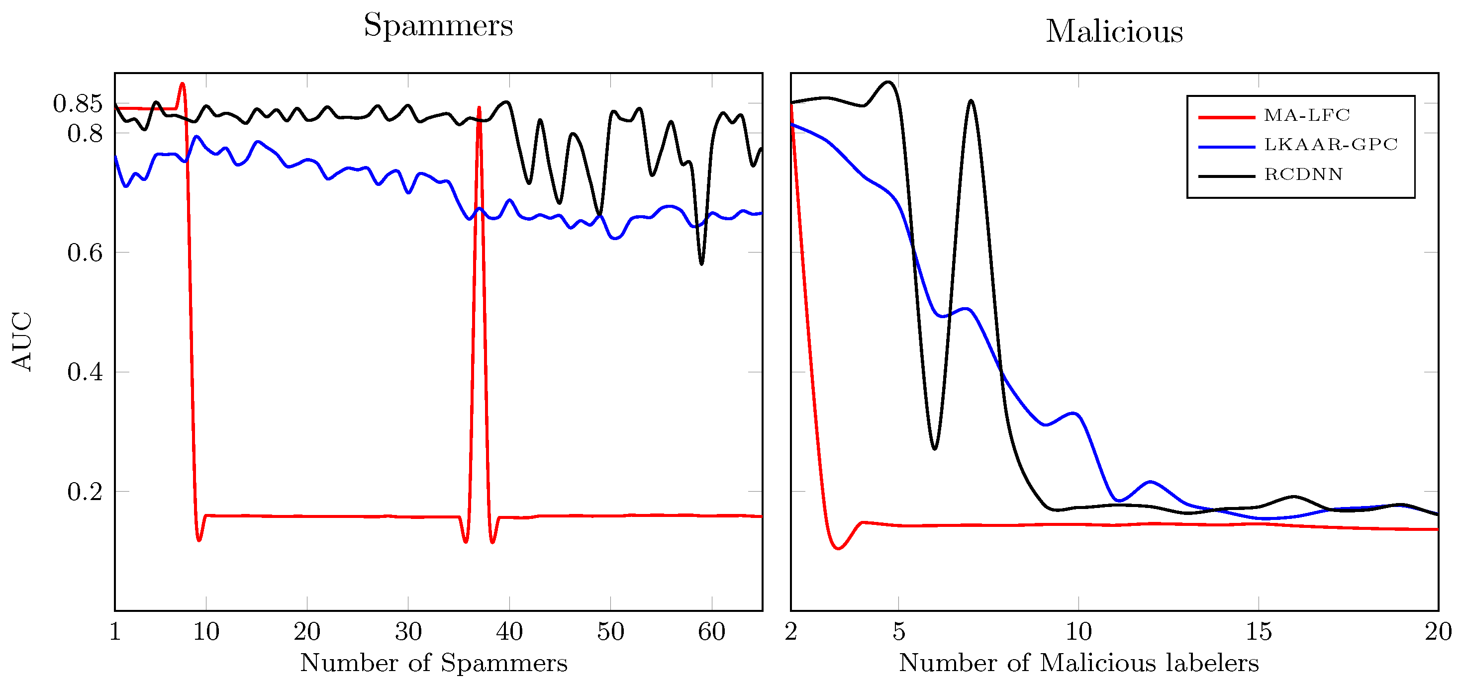
This paper introduces a novel regularized chained deep neural network classifier, termed RCDNN, to deal with multiple annotator scenarios. Our method is built based on the ideas of the chained Gaussian processes [25], where each parameter in a multi-labeler likelihood is modeled by using the outputs of a deep neural network. In such a way, RCDNN codes the annotators’ expertise as a function of the input data and the dependencies among the labelers from the last hidden layer’s weights. Besides, l1, l2, and Monte-Carlo Dropout regularization strategies are coupled within our RCDNN architecture and predictor to contract the over-fitting challenge of deep models. The proposal is tested using different scenarios concerning the provided annotations: synthetic, semi-synthetic, and real-world experts. According to the results, RCDNN achieves robust predictive properties for the studied datasets even in the presence of Spammers and Malicious labelers, outperforming state-of-the-art methods while providing an estimation of each labeler’s reliability and the dependencies among annotators.

As future work, extending RCDNN for regression tasks is an exciting research line, i.e., based on the model introduced in [12]. Next, the authors plan to use other deep structures, i.e., Convolutional and Recurrent layers and different activation functions, to apply our approach in more complex tasks such as computer vision or natural language processing. Finally, as RCDNN was tested on the Western dataset, which comprises building a system to diagnose an engine’s status, the authors plan to focus on that topic to build an automatic system to identify internal combustion engines’ conditions from multiple annotators.

References

1. Gil-Gonzalez, J.; Orozco-Gutierrez, A.; Alvarez-Meza, A. Learning from multiple inconsistent and dependent annotators to support classification tasks. Neurocomputing 2021, 423, 236–247. [Google Scholar] [CrossRef]
2. Raykar, V.C.; Yu, S.; Zhao, L.H.; Valadez, G.H.; Florin, C.; Bogoni, L.; Moy, L. Learning from crowds. J. Speech Lang. Hear. Res. 2010, 11, 1297–1322. [Google Scholar]
3. Liu, Y.; Zhang, W.; Yu, Y. Truth inference with a deep clustering-based aggregation model. IEEE Access 2020, 8, 16662–16675. [Google Scholar]
4. Snow, R.; O’Connor, B.; Jurafsky, D.; Ng, A. Cheap and fast—but is it good? Evaluating non-expert annotations for natural language tasks. In Proceedings of the 2008 Conference on Empirical Methods in Natural Language Processing, Honolulu, HI, USA, 25–27 October 2008; pp. 254–263. [Google Scholar]
5. Zhang, J.; Wu, X.; Sheng, V.S. Learning from crowdsourced labeled data: A survey. Artif. Intell. Rev. 2016, 46, 543–576. [Google Scholar] [CrossRef]
6. Sung, H.E.; Chen, C.K.; Xiao, H.; Lin, S.D. A Classification Model for Diverse and Noisy Labelers. In Pacific-Asia Conference on Knowledge Discovery and Data Mining; Springer: Berlin/Heidelberg, Germany, 2017; pp. 58–69. [Google Scholar]
7. Tao, D.; Cheng, J.; Yu, Z.; Yue, K.; Wang, L. Domain-weighted majority voting for crowdsourcing. IEEE Trans. Neural Netw. Learn. Syst. 2018, 30, 163–174. [Google Scholar] [CrossRef]
8. Rizos, G.; Schuller, B.W. Average Jane, Where Art Thou?–Recent Avenues in Efficient Machine Learning Under Subjectivity Uncertainty. In International Conference on Information Processing and Management of Uncertainty in Knowledge-Based Systems; Springer: Berlin/Heidelberg, Germany, 2020; pp. 42–55. [Google Scholar]
9. Ruiz, P.; Morales-Álvarez, P.; Molina, R.; Katsaggelos, A.K. Learning from crowds with variational Gaussian processes. Pattern Recognit. 2019, 88, 298–311. [Google Scholar] [CrossRef]
10. Zhang, J.; Wu, X.; Sheng, V.S. Imbalanced multiple noisy labeling. IEEE Trans. Knowl. Data Eng. 2014, 27, 489–503. [Google Scholar] [CrossRef]
11. Dawid, A.; Skene, A. Maximum likelihood estimation of observer error-rates using the EM algorithm. Appl. Stat. 1979, 20–28. [Google Scholar] [CrossRef]
12. Groot, P.; Birlutiu, A.; Heskes, T. Learning from multiple annotators with Gaussian processes. In International Conference on Artificial Neural Networks; Springer: Berlin/Heidelberg, Germany, 2011; pp. 159–164. [Google Scholar]
13. Xiao, H.; Xiao, H.; Eckert, C. Learning from multiple observers with unknown expertise. In Pacific-Asia Conference on Knowledge Discovery and Data Mining; Springer: Berlin/Heidelberg, Germany, 2013; pp. 595–606. [Google Scholar]
14. Rodrigues, F.; Pereira, F.C.; Ribeiro, B. Gaussian Process Classification and Active Learning with Multiple Annotators. In Proceedings of the 31st International Conference on Machine Learning, Bejing, China, 22–24 June 2014; pp. 433–441. [Google Scholar]
15. Morales-Álvarez, P.; Ruiz, P.; Coughlin, S.; Molina, R.; Katsaggelos, A.K. Scalable Variational Gaussian Processes for Crowdsourcing: Glitch Detection in LIGO. arXiv 2019, arXiv:1911.01915. [Google Scholar]
16. Gil-Gonzalez, J.; Alvarez-Meza, A.; Orozco-Gutierrez, A. Learning from multiple annotators using kernel alignment. Pattern Recognit. Lett. 2018, 116, 150–156. [Google Scholar] [CrossRef]
17. Morales-Álvarez, P.; Ruiz, P.; Santos-Rodríguez, R.; Molina, R.; Katsaggelos, A.K. Scalable and efficient learning from crowds with Gaussian processes. Inf. Fusion 2019, 52, 110–127. [Google Scholar] [CrossRef]
18. Rodrigues, F.; Pereira, F.; Ribeiro, B. Sequence labeling with multiple annotators. Mach. Learn. 2014, 95, 165–181. [Google Scholar] [CrossRef] [Green Version]
19. Albarqouni, S.; Baur, C.; Achilles, F.; Belagiannis, V.; Demirci, S.; Navab, N. Aggnet: Deep learning from crowds for mitosis detection in breast cancer histology images. IEEE Trans. Med. Imaging 2016, 35, 1313–1321. [Google Scholar] [CrossRef] [PubMed]
20. Rodrigues, F.; Pereira, F.C. Deep learning from crowds. In Proceedings of the Thirty-Second AAAI Conference on Artificial Intelligence, New Orleans, LA, USA, 2–7 February 2018. [Google Scholar]
21. Venanzi, M.; Guiver, J.; Kazai, G.; Kohli, P.; Shokouhi, M. Community-based Bayesian aggregation models for crowdsourcing. In Proceedings of the 23rd International Conference on World Wide Web, Seoul, Korea, 7–11 April 2014; ACM: New York, NY, USA, 2014; pp. 155–164. [Google Scholar]
22. Tang, W.; Yin, M.; Ho, C.J. Leveraging Peer Communication to Enhance Crowdsourcing. In The World Wide Web Conference; ACM: New York, NY, USA, 2019; pp. 1794–1805. [Google Scholar]
23. Zhang, P.; Obradovic, Z. Learning from inconsistent and unreliable annotators by a Gaussian mixture model and Bayesian information criterion. In Joint European Conference on Machine Learning and Knowledge Discovery in Databases; Springer: Berlin/Heidelberg, Germany, 2011; pp. 553–568. [Google Scholar]
24. Hahn, U.; von Sydow, M.; Merdes, C. How Communication Can Make Voters Choose Less Well. Top. Cogn. Sci. 2018, 11, 194–206. [Google Scholar] [CrossRef] [PubMed]
25. Saul, A.; Hensman, J.; Vehtari, A.; Lawrence, N. Chained Gaussian processes. In Proceedings of the 19th International Conference on Artificial Intelligence and Statistics, Cadiz, Spain, 9–11 May 2016; pp. 1431–1440. [Google Scholar]
26. Rodrigo, E.; Aledo, J.; Gámez, J. Machine learning from crowds: A systematic review of its applications. Wiley Interdiscip. Rev. Data Min. Knowl. Discov. 2019, 9, e1288. [Google Scholar] [CrossRef]
27. Yan, Y.; Rosales, R.; Fung, G.; Subramanian, R.; Dy, J. Learning from multiple annotators with varying expertise. Mach. Learn. 2014, 95, 291–327. [Google Scholar] [CrossRef]
28. Wang, X.; Bi, J. Bi-convex optimization to learn classifiers from multiple biomedical annotations. IEEE ACM Trans. Comput. Biol. Bioinform. 2016, 14, 564–575. [Google Scholar] [CrossRef]
29. Zhu, T.; Pimentel, M.A.; Clifford, G.D.; Clifton, D.A. Unsupervised Bayesian Inference to Fuse Biosignal Sensory Estimates for Personalising Care. IEEE J. Biomed. Health 2019, 23, 47. [Google Scholar] [CrossRef]
30. Rodrigues, F.; Lourenco, M.; Ribeiro, B.; Pereira, F. Learning supervised topic models for classification and regression from crowds. IEEE Trans. PAMI 2017, 39, 2409–2422. [Google Scholar] [CrossRef] [Green Version]
31. Hua, G.; Long, C.; Yang, M.; Gao, Y. Collaborative Active Visual Recognition from Crowds: A Distributed Ensemble Approach. IEEE Trans. Pattern Anal. Mach. Intell. 2018, 40, 582–594. [Google Scholar] [CrossRef]
32. Rodrigues, F.; Pereira, F.; Ribeiro, B. Learning from multiple annotators: Distinguishing good from random labelers. Pattern Recognit. Lett. 2013, 34, 1428–1436. [Google Scholar] [CrossRef]
33. Géron, A. Hands-on Machine Learning with Scikit-Learn, Keras, and TensorFlow: Concepts, Tools, and Techniques to Build Intelligent Systems; O’Reilly Media: Sebastopol, CA, USA, 2019. [Google Scholar]
34. Hernández-Muriel, J.A.; Bermeo-Ulloa, J.B.; Holguin-Londoño, M.; Álvarez-Meza, A.M.; Orozco-Gutiérrez, Á.A. Bearing Health Monitoring Using Relief-F-Based Feature Relevance Analysis and HMM. Appl. Sci. 2020, 10, 5170. [Google Scholar] [CrossRef]
35. Arias, J.; Godino, J.; Gutiérrez, J.; Osma, V.; Sáenz, N. Automatic GRBAS assessment using complexity measures and a multiclass GMM-based detector. In Proceedings of the 7th International Workshop on Models and Analysis of Vocal Emissions for Biomedical Applications (MAVEBA 2011), Florence, Italy, 25–27 August 2011; pp. 111–114. [Google Scholar]
36. Gil, J.; Álvarez, M.; Orozco, Á. Automatic assessment of voice quality in the context of multiple annotations. In Proceedings of the 2015 37th Annual International Conference of the IEEE Engineering in Medicine and Biology Society (EMBC), Milan, Italy, 25–29 August 2015; pp. 6236–6239. [Google Scholar]
37. Yan, Y.; Rosales, R.; Fung, G.; Schmidt, M.W.; Valadez, G.H.; Bogoni, L.; Moy, L.; Dy, J.G. Modeling annotator expertise: Learning when everybody knows a bit of something. In Proceedings of the Thirteenth International Conference on Artificial Intelligence and Statistics, Sardinia, Italy, 13–15 May 2010; pp. 932–939. [Google Scholar]
38. Fawcett, T. An introduction to ROC analysis. Pattern Recognit. Lett. 2006, 27, 861–874. [Google Scholar] [CrossRef]
39. Demšar, J. Statistical comparisons of classifiers over multiple data sets. J. Mach. Learn. Res. 2006, 7, 1–30. [Google Scholar]
40. Bishop, C. Pattern Recognition and Machine Learning; Springer: Berlin/Heidelberg, Germany, 2006. [Google Scholar]
Figure 1. Regularized chained deep neural network (RCDNN) classifier for multiple annotators. J = K + R outputs are used to model the hidden ground truth label (as 1-K coding) and each expert’s reliability.
Applsci 11 05409 g001
Figure 2. RCDNN architecture details. ϵ s stands for dense layer. ϵ 1 holds a linear activation, ϵ 2 includes a tanh-based activation, and ϵ 3 and ϵ 4 output the hidden ground truth label and the annotator’s reliability fixing a softmax and a sigmoid activation, respectively.
Applsci 11 05409 g002
Figure 3. RCDNN’s decision boundaries for the 2D-PCA Iris dataset (synthetic scenario). AUC = 0.9837 . The point’s color stands for the Iris dataset classes. P C A 1 and P C A 2 stand for the first and second PCA-based projections.
Applsci 11 05409 g003
Figure 4. RCDNN-based annotators performance (reliability) estimation for the synthetic experiments (2D PCA Iris data). In the first column (from top to bottom), the simulated accuracy for each annotator is presented based on Equation (10). The second column shows (from top to bottom) the estimated annotators’ reliability ( λ r ).
Applsci 11 05409 g004
Figure 5. Target and estimated annotators dependencies for the synthetic 2D PCA Iris dataset. In the left, the Pearson correlation coefficients (absolute value) from simulated accuracies (experts reliability) in matrix A of Equation (10) are shown. In the right, the dependencies among the annotators estimated from the RCDNN ϵ 4 layer’ weights are displayed.
Applsci 11 05409 g005
Figure 6. Receiver operating characteristic (ROC) plot for the annotators simulated within the spammers and malicious scenario. Blue dots indicate the basis annotators. Red dots show extra annotators with parameters R e = 65 , and p r = 0.5 . Green dots specify extra labelers with R e = 20 , and p r = 0.6 . We notice that annotators located in dashed line vicinity are considered Spammers. Similarly, labelers above the dashed line are regarded as good annotators; conversely, labelers located below such a line are malicious annotators.
Applsci 11 05409 g006
Figure 7. MA-LFC, LKAAR-GPC, and RCDNN performance (AUC) as a function of the number of labelers (spammers and malicious annotators).
Applsci 11 05409 g007