Article

Numerical Study of the Influence of the Inlet Turbulence Length Scale on the Turbulent Boundary Layer

1
National Institute of Meteorological Sciences Operational Systems Development Department, 145, Seohojungang-ro, Seogwipo-si 63568, Jeju-do, Korea
2
School of Mechanical Engineering, Pusan National University, 2, Busandaehak-ro 63 beon-gil, Geumjeong-gu, Busan 46241, Korea
*
Author to whom correspondence should be addressed.
Appl. Sci. 2021, 11(11), 5177; https://doi.org/10.3390/app11115177
Submission received: 20 April 2021 / Revised: 15 May 2021 / Accepted: 27 May 2021 / Published: 2 June 2021
(This article belongs to the Topic Dynamical Systems: Theory and Applications)

Abstract

:
In the past half century, large eddy simulations (LESs) have played an important role in turbulent flow simulation and improving the performance of computing technology. To generate a fully developed turbulent boundary layer in the channel domain using LES, suitable inflow conditions along with turbulent characteristics are required. This study aimed to clarify the effect of the integral length scale on the generation of turbulent boundary layers. To accomplish this, an artificially created boundary layer was imposed on the inlet section, which gradually evolved into a fully developed turbulent boundary layer flow inside the numerical domain. In this study, the synthetic inflow method, which is a commonly employed technique, was used by imposing the spatial and temporal correlation between two different points on the inlet section. In addition, we conducted parametric length scale studies on the inlet section and compared our results with existing data. The results showed that the larger length scales in the spanwise direction were not only effective in achieving the target shape of a fully developed turbulent boundary layer, but also developed it faster than the smaller length scales.

1. Introduction

In a variety of engineering and basic scientific area, the turbulent boundary layers over smooth and rough wall surfaces have long been discussed and reported. It is usually related with an increase in momentum transport, for example, see the literatures (Kovasznay [1], Willmarth [2], Kline et al. [3], Sreenivasan [4] , Kline and Robinson [5], and Cermak and Cochran [6]). Depending on the shape and height of the surface roughness, the flow field could be substantially different in terms of the mean velocity and turbulence statistics (see Rachele et al. [7], Rachele et al. [8] and Raupach et al. [9]) Regarding the details of turbulent boundary layer on the surface, there have been more literatures (Meroney [10], Kolmogorov [11], Prandtl [12], Tennekes and Lumley [13], Hunt [14], and Sun and Mahrt [15]).
In direct numerical simulation (DNS), all scales ranging from the smallest scales, where the dissipation of the turbulence kinetic energy into thermal energy takes place (termed the Kolmogorov length scale), up to the largest scales (typically defined by the characteristic length of the flow configuration being considered) are resolved both in space and time. Therefore, DNS requires enormous computational efforts. DNS studies are still limited to the flow problems with small Reynolds numbers and simple geometries. On the other hand, regarding large eddy simulation (LES), only the large scales are resolved, and the effects of the smallest scales are modeled. This is because the large-scale eddies are known to be largely affected by the boundary conditions and therefore should be computed, but small scales are largely independent of the flow geometry and tend to be homogeneous and isotropic, irrespective of the geometry being considered, and, therefore, can be easily modelled. Therefore, LES requires less computational effort than that for DNS, and the computational requirements of the LES remain rather high for the optimization of complicated processes where a large number of computations need to be performed.
The most direct method of generating a well-developed turbulent boundary layer is to simulate a laminar inflow and allow it to develop spatially over a suitably long domain, i.e., over a hundred times the thickness of the eventual boundary layer depth of interest. However, even this “simple” method would present difficulties associated with ensuring the correct surface conditions, such as the length scale and wall treatment. Further, the computational cost would be very high. Alternatively, using a time-evolving large eddy simulation (LES) or direct numerical simulation (DNS) with a periodic (Lee et al. [16], Keating et al. [17], Lim et al. [18], Lim et al. [19]) or a “modified periodic” (Lund and Wu [20]) boundary condition, the inlet–outlet boundary condition can be used to generate the appropriate turbulent flow. For the latter, Lim et al. [18] used a sort of “precursor simulation”, in which the velocity field at an appropriate downstream station is stored and imposed in a suitably re-scaled form as the inflow data for the primary computation. The precursor simulation generates a realistic turbulent flow field. However, it is also expensive and has limitations, such as its applicability to simple geometries only. Therefore, it is difficult to determine the usefulness of such a method in actual urban-type scenarios.
Procedures that are based on proper orthogonal decomposition (Druault et al. [21], Johansson and Andersson [22], Perret et al. [23]) may be less expensive than the above methods for the generation of inflow data provided that there are appropriate DNS/LES (Johansson and Andersson [22]) or experimental datasets (Druault et al. [21], Perret et al. [23]) available for processing in order to obtain the most energetic modes, with an appropriate set of time-dependent projection coefficients that provide the phase information. The reconstructed inflow data for later LES/DNS are “almost realistic”. However, experimental databases suffer from either low spatial resolution, which is common in measurements from hot-wire or laser Doppler anemometry (Druault et al. [21]), or low temporal resolution, as obtained from measurements using particle-image velocimetry (Perret et al. [23]).
Special treatment must then be applied to resolve the issues pertaining to its low resolution. Consequently, such approaches are generally suitable only for very specific cases; synthetic turbulence generation is another option and is of particular interest when only limited turbulence statistics data are available. Hanna et al. [24] generated one-dimensional (1D) time series of inflow data based on an exponential correlation function to simulate flows over an array of cubes using LES. The time series were tailored to provide the required time scale and turbulence intensities, and the subsequent LES was able to reproduce the main characteristics of the measurements. The merit of that method is its very high efficiency; however, its accuracy is seriously limited because no spatial correlation was imposed at the inlet.
Because of the features of the atmospheric boundary layer flows as an inflow condition, one of the representative studies would be the work of Xie and Castro [25] and Xie and Castro [26]. They used the urban boundary layer flows, which should have a high Reynolds number, and fully developed turbulence driven by large-scale motions. They used a digital filter-based method, which allows spatially varying turbulence scales on non-uniform grids to be imposed at the inlet. It was developed independent of the works of Mare et al. [27], Veloudis et al. [28], whose methods were similar in some respects and have already been used elsewhere (Jarrin et al. [29]). There are some more literatures (Renard et al. [30], Gupta and Kalita [31], Barragy and Carey [32], Bennacer et al. [33], Kareem and Gao [34]).
Therefore, this study investigated the flow characteristics in a channel with a smooth wall by imposing synthetic inflow data having a varying length scale. Various inflow length scales were imposed to examine their effect on the whole flow domain with the aim of observing the relationship between the length scale and the development of the turbulent boundary layer. This paper is organized as follows: In Section 2, the governing equation and synthetic inflow generation using the digital filtering method for the LES inlet condition are introduced and summarized. This is confirmed by making a comparison with the turbulent statistics from an existing DNS database. In Section 3, the synthetic inflow generation technique was validated by the simulation of a smooth wall-bounded channel flow. Furthermore, the characteristics of the turbulent boundary layers simulated by LES using inlet data imposed by the synthetic inflow generation were analyzed. In addition, the effects of the inlet length scales on the development of a flow structure inside the flow domain were also investigated. Finally, Section 4 concludes this study.

2. Numerical Analysis

2.1. Governing Equation

To resolve the incompressible flow, we must estimate the flow structure for a wide range of scales. The DNS method can resolve a wide range of scales, from large ones to the Kolmogorov, which is the smallest scale. However, until now, its computational cost has been too high for it to be used as a design tool. LESs resolve only a large scale of motion, and the effect of smaller scales is modeled by the sub-grid scale (SGS) modeling.
In LESs, the governing equations for a large eddy are applied after a spatial filtering operation. The spatial filtering operation is given by:
f ¯ ( x ) = G ( x x ) f ( x ) d x
where f is a turbulent field and G is a spatial filter.
The continuity and momentum equations for incompressible flows are obtained by filtering the Navier–Stokes equations. The filtered Navier–Stokes equations are given by:
u ¯ i x i = 0
u ¯ i t + u ¯ j u ¯ i x j = 1 ρ p ¯ x i + 2 ν x j S ¯ i j τ i j r x j
where τ i j r is the residual stress tensor. τ i j r is given by:
τ i j r = u i u j ¯ u ¯ i u ¯ j
In Equation (4), the residual stress tensor is unknown and should be modeled. The eddy viscosity Boussinesq hypothesis is used for modeling the residual stress tensor as follows:
τ i j r = 2 μ t S ¯ i j + 1 3 τ k k δ i j
where μ t is the turbulent viscosity of the sub-grid scale. The isotropic part of δ i j is added to the filtered static pressure term without being modeled. In Equation (5), S ¯ i j is the filtered rate of the strain tensor and is defined by:
S ¯ i j = 1 2 u ¯ i x j + u ¯ j x i
The Smagorinsky–Lilly model was used as a subgrid-scale model. In this study, the Smagorinsky constant C s was set to 0.065 (Moin and Kim [35]).

2.2. Modeling of the Inflow Generator

We investigated a synthetic inflow generator having a variety of length scales, which was based on Xie and Castro’s method (Xie and Castro [26]) (XC). In this section, we present a brief review of the XC model. The XC model imposes correlations using an exponential function to satisfy the prescribed space and time correlations. The instantaneous value of the velocity u i may be written as:
u i = u ¯ i + a i j ψ j
where u ¯ i is the mean and a i j ψ j is the fluctuating part of u i , which is called Reynolds decomposition. The fluctuating part can be separated into two parts, a i j , which is the amplitude tensor, and ψ j , which is the unscaled fluctuation with zero mean ( ψ ¯ j = 0 ), a unit variance ( ψ j ψ j ¯ = 1 ), and zero covariance with the other distributions ( ψ j ψ j ¯ = 0 , i j ). The term a i j using Reynolds stress R i j is the Cholesky decomposition of the Reynolds stress by Le and Moin [36] as follows,
a i j = R 11 0 0 R 21 R 22 a 21 2 0 R 31 / a 11 ( R 32 a 21 a 31 / a 22 R 33 a 31 2 a 32 2
where R i j is the Reynolds stress tensor obtained from the experimental or previously calculated numerical simulation data. If the boundary layer is homogeneous in the lateral direction, R 31 = R 32 = 0 ; therefore, a 31 and a 32 can be removed.
The synthetic inflow generation technique using digital filtering aims to find the unscaled fluctuation ( ψ j ), which is a one-dimensional number sequence with zero mean, unit variance, and spatial correlation. The correlations in the most turbulent shear flow have similar features. The advantage of the correlation function is that it approximates the relation of two different points to the form of an exponential function. The exponential function is exp ( π r / β L , where β = 2 . However, in the equation, β is not clearly defined, and its function remains unclear. In this study, the exponential function was carefully tested and subsequently modified. The modified exponential function is expressed as follows (Kim et al. [37]):
R ( r , 0 , 0 ) = e x p ( π r 4 L )
where L is the integral length scale and r is a 1D random number sequence with zero mean. The filter is designed to process a series of random numbers using an exponential function. Taking a filter coefficient and a series of random numbers into account, the velocity field is derived as follows:
ψ m = j = N N b j r m + j
where ψ m , b j , and r m are the velocity field, filter coefficient, and a series of random numbers with zero mean ( r ¯ m = 0 ), respectively, and unit variance ( r m r m ¯ = 1 ). In addition, the integral length scale (L) can be considered as a multiple of the grid size ( Δ x ) and expressed as L = n Δ x . In addition, N is determined by the integral length scale. The relation between N and n was also carefully tested for N 2 n , and finally, N = 2 n was accepted. In this study, the variation of the length scale was made in the inlet section. Using Equations (9) and (10), the filter coefficient b j could be defined as shown in Equation (11).
b j = ( b ˜ j ) / k = N N b ˜ k 2 1 / 2 , b ˜ j = e x p π | j | 2 n
Based on these equations, one-dimensional data satisfying the required length scale L, mean ψ ¯ m = 0 , and variance ψ m ψ m ¯ = 1 can be obtained. The filter coefficient for a two-dimensional (2D) plane can be obtained by the convolution of two 1D filter coefficients, b j k = b j b k . It is expressed as follows:
ψ m , l = j = N N k = N N b j k r m + j , l + k
In the first time step, the velocity data of a plane are generated by applying the filter to the random number on the 2D plane. The data ψ j ( t , y , z ) of the 2D plane are set to have a constant length scale, L i = n i Δ x i , in the vertical direction and in the spanwise direction. To impose a more precise length scale, it is also possible to divide the region of the inlet plane and apply different length scales at each region. The time scale should be considered for the application of the plane velocity field data for the next time step. Based on Taylor’s hypothesis, the Lagrangian time scale can be expressed as follows:
T = L / u ¯
where L is the length scale and u ¯ is the local mean velocity. In addition, the Eulerian time scale, T, can be obtained from experimental or previous numerical analyses. The velocity of the next time step can be calculated by Equation (14) using the velocity at the previous time step.
ψ i ( t + Δ t , y , z ) = ψ i ( t , y , z ) e x p π Δ t 4 T + ϕ i ( t , y , z ) 1 e x p π Δ t 2 T 0.5
where ϕ i is obtained using a new set of random data; however, ψ i is the plane velocity field data of the current or next time step and T is a constant value for the entire inlet plane representing the Eulerian time scale. Note that ϕ i is fully random in time, its variance is unity, and it is an independent variable from ψ i ( t , y , z ) .

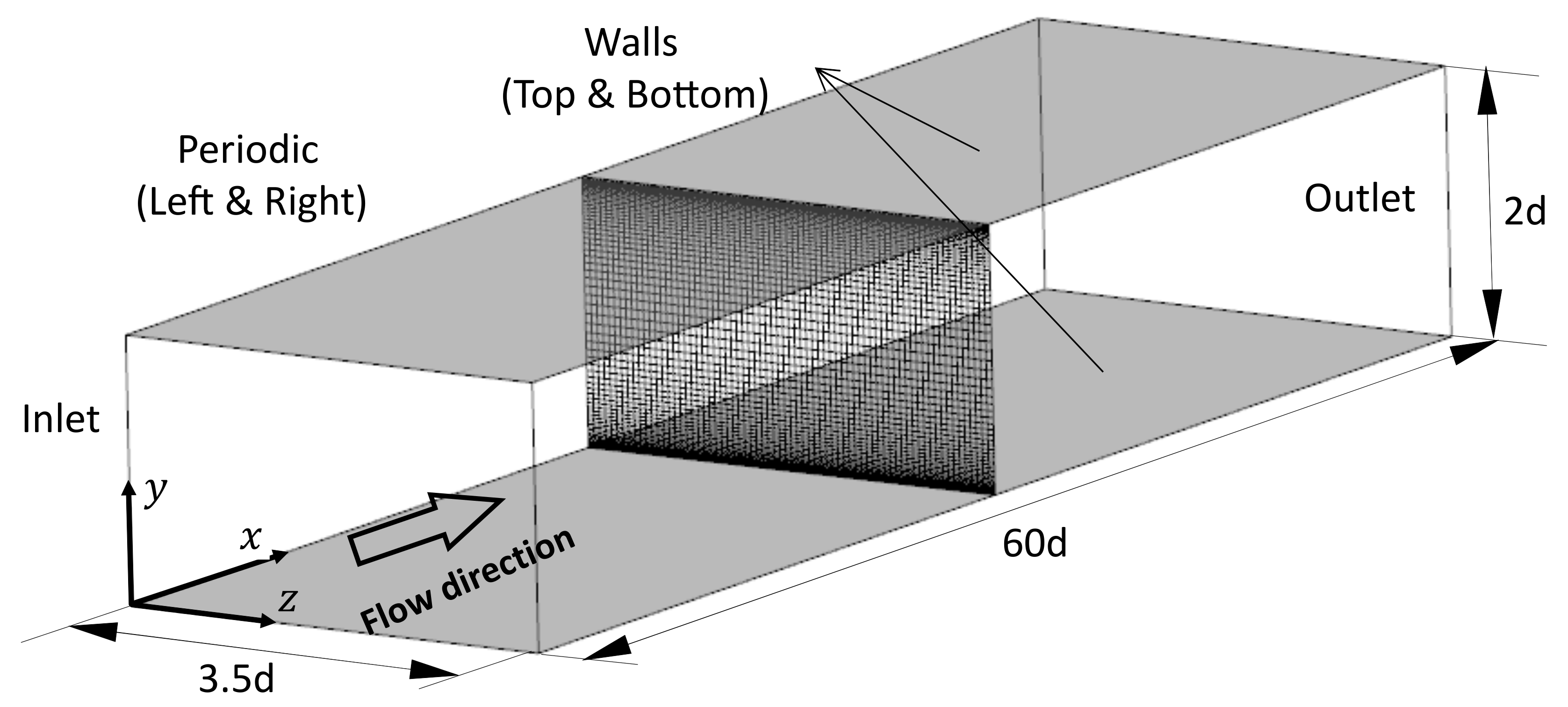
2.3. Implementation of the Boundary Condition and Inflow Length Scale

In this study, a hexahedral grid system was used for the numerical simulation of making fully developed turbulent flow. To improve the convergence efficiency in the solution of the governing equations, a stretch mesh was used so that the grid was concentrated on the wall surface, and the resolution was sufficiently high close to the wall, but coarse at the far field from the wall. The Reynolds number ( R e τ ) on the smooth wall-bounded channel flow was 150 based on the friction velocity ( u τ ) and the half height (d) of the channel. The size of the whole computational domain was 60 d × 2 d × 3.5 d in the streamwise (x), wall normal (y), and spanwise (z) directions, respectively. The number of cells in the whole domain was approximately 2.5 million, as shown in Figure 1. To improve the convergence of the analysis, a stretch mesh satisfying y + < 1 in the first cell center was considered for the wall-normal direction. For the x and z directions, uniform meshes were used, and the resolutions were Δ x + = 15 , Δ z + = 7.5 . The number of cells in each direction was 600 × 60 × 70 in the x, y, and z directions, respectively. All statistics were averaged by 40 t * , where t * = t u τ / d is a non-dimensional time. Averaging for the statistical analysis was performed after the initialization period of 400 t * . The Smagorinsky subgrid-scale model was adopted with a constant c s = 0.065 (Moin and Kim [35]). The time step satisfies the condition that the CFL number should be smaller than one. The corresponding Δ t * = Δ t × u τ / δ = 0.001 . A second-order implicit scheme was used for time discretization, and a second-order central difference scheme was used for spatial discretization. Furthermore, the transient incompressible flow solver was used, and the PISO algorithm was adopted as the velocity–pressure coupling scheme. The PRESTO algorithm was used as a discretization technique for pressure (Solozano et al. [38]).
The boundary conditions of this channel flow were: a no-slip condition on the top and bottom walls, a periodic boundary condition in the lateral direction, and a zero-gradient condition with no diffusion of all the flow variables on the outlet. The synthetic turbulence obtained by the synthetic inflow generator was interpolated into the cell center of the inlet plane. The statistical information of turbulent flow, including the first and second moment statistics and the integral length scales used as input parameters to generate the synthetic inflow, were obtained from the DNS database that analyzed the plane channel flow (Moin and Kim [35]). The integral length scale L i was obtained using Equation (15) with a two-point correlation and R ( x i ) in the DNS database.
L i = 0 R ( x i ) d x i , i = 1 , 2 , 3
Figure 2 shows the length scale obtained from the DNS database and the simplified length scale applied to the synthetic inflow generation. Figure 2a shows the distribution of the streamwise direction length scale, L x , along the wall-normal direction.
If the relative turbulence intensities are sufficiently low, according to Taylor’s hypothesis, the length scale can be determined by the local mean velocity u ¯ and the Eulerian time scale T. Therefore, L x ( y ) = T × u ¯ ( y ) is applicable (Taylor [39]). In the equation, T is a constant, and the local mean velocity in the streamwise direction increases with the distance from the wall, while the streamwise length scale also becomes large. In this study, the turbulence intensity of the flow simulation was smaller than 0.3, and Taylor’s hypothesis can therefore be applied across the entire domain. However, the streamwise length scale obtained from the actual DNS was highest close to the wall and gradually decreased in the freestream. To impose a precise streamwise length scale of actual DNS data as the inlet condition, the three-dimensional (3D) domain should be considered when generating the fluctuating part, ψ i . The advantage of the inflow generation technique considered in this study is that it can generate efficient inlet velocity field data at every time step only on the 2D plane, while matching the second-order turbulent statistics obtained from the experiment or a previously calculated simulation. Figure 2b shows the length scale for the y and z directions. Notably, there are no DNS data of a length scale in the wall-normal direction (y) in the existing literature. Therefore, because it is inhomogeneous for the wall-normal direction, we assumed in the study that L y = 0.67 L z for the length scale in the y direction (see Iwamoto et al. [40]). As mentioned above, the entrance plane can be divided into several sections, and different values of L y and L z were applied to each section.

2.4. Variation of Inflow Length Scale

In this study, the flow characteristics were observed with variations in the integral length scales at the inlet section. As mentioned earlier, the streamwise local length scale, L x ( y ) , is determined by the local mean velocity, u ¯ ( y ) , and the constant time scale, T, where the constant T could be obtained by L x and u ¯ at y / d = 1 . The spanwise length scale could be applied as a multiple of L z * , where L z * is the reference spanwise length scale, which is equivalent to the value L z used in Figure 2. To observe the effect of the L z distribution on the flow field, this study chose several different values, such as 0 L z * (white noise), 0.15 L z * , 0.3 L z * , 0.5 L z * , 2 L z * , and 3 L z * (see Table 1). To achieve a precise matching with the L z * distribution of the existing DNS database, in the length scales L z * , the domain needed to be divided into three different zones. These zones were separated in several salient positions at y / d = 0.1 , 0.2 . Table 1 presents the configuration of each case depending on the size of the length scale in each zone. For instance, Case 02 did not consider the length scale in the inlet condition, whereas Cases 01, 07, and 08 had a uniform spanwise length scale in L z . Besides, to observe the effect of different length scales on different zones, Cases 03, 04, 05, and 06 would play an important role, in addition to studying the variation of flow statistics based on length scales. Depending on the location of the length scale, the zone was divided at y / d = 0.1 and 0.2 . In particular, Cases 07 and 08 had length scales that were two and three times larger, respectively, than that of Case 01 for all the streamwise, vertical, and spanwise directions.

2.5. Filtering Process and Correlation

This study adopted the filtering process in which random data are filtered and correlated to obtain fluctuating data in ψ m . When the series of random numbers was filtered through the synthetic inflow model used in this study, the filtered velocity field data, which were similar to the fluctuating part of the flow, were obtained. To apply this algorithm to the synthetic inflow generator, the velocity field data were first generated in a 2D equi-spaced uniform mesh and then interpolated into a non-uniform mesh with the aim of fitting it into the more realistic inlet domain as an inlet condition.
Figure 3 compares the DNS database with the data from the synthetic inflow generator for the mean and turbulent statistics. The non-dimensional parameters used here can be defined as follows:
y + = u τ y ν , u + = u u τ , < u i u i > + = Σ ( u i u i ) u τ
In the figure, the ordinate axis shows the non-dimensional mean and stress profiles, and the abscissa represents the non-dimensional distance from the wall ( y + ). In the mean velocity profile u + , the current result agreed well with the overall range of the domain, such as the law of the wall at y + < 5 and the logarithmic law at y + > 30 . In addition, it can be seen that the axial and shear stresses from the synthetic inflow generator were in good agreement with the DNS data. In this study, the mean velocity log law was applied as:
U u * = 1 κ l n y d y 0
where u * and d are the friction velocity ( τ w a l l / ρ ) and “zero plane displacement”, respectively.

3. Results and Discussion

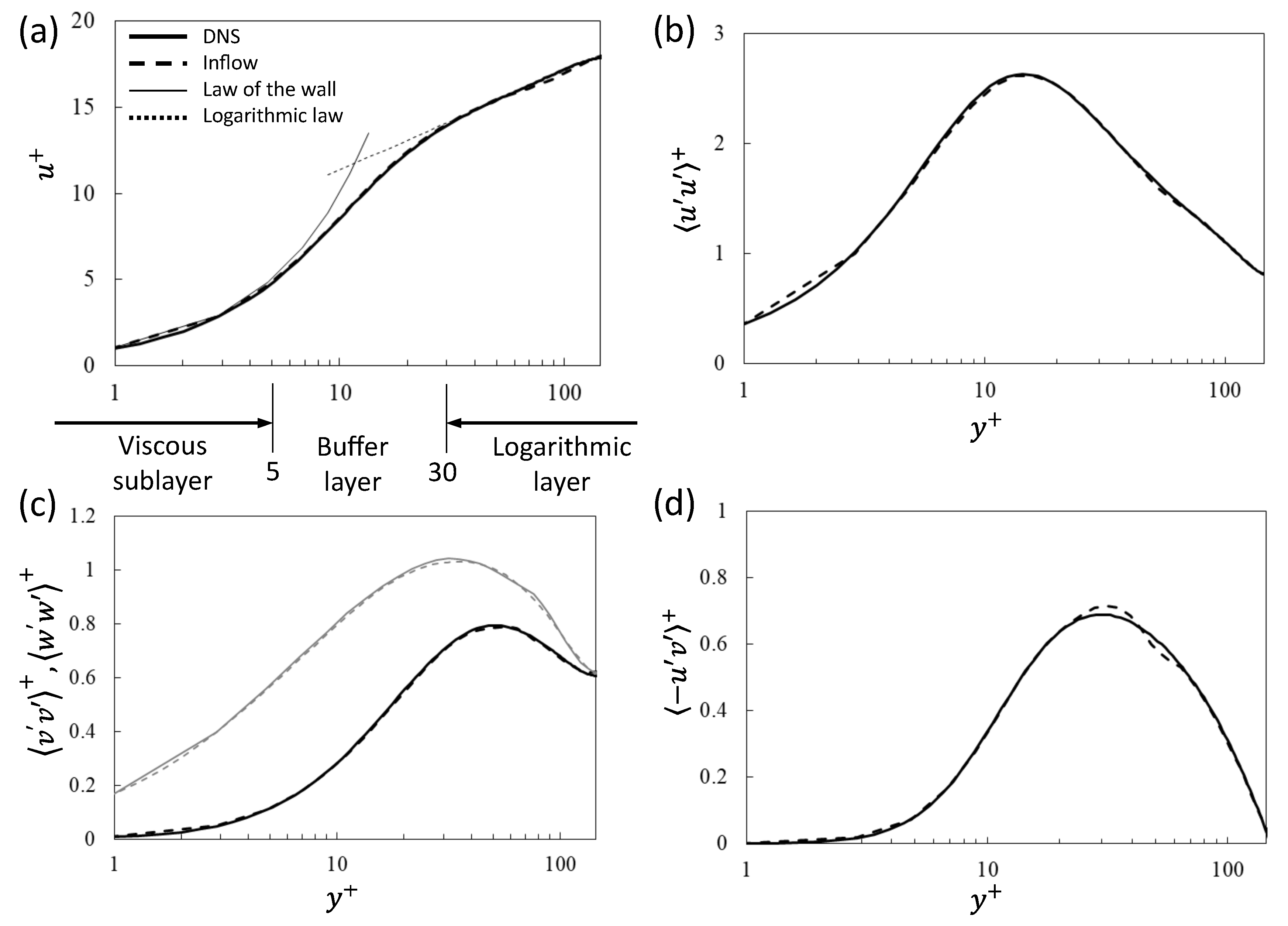
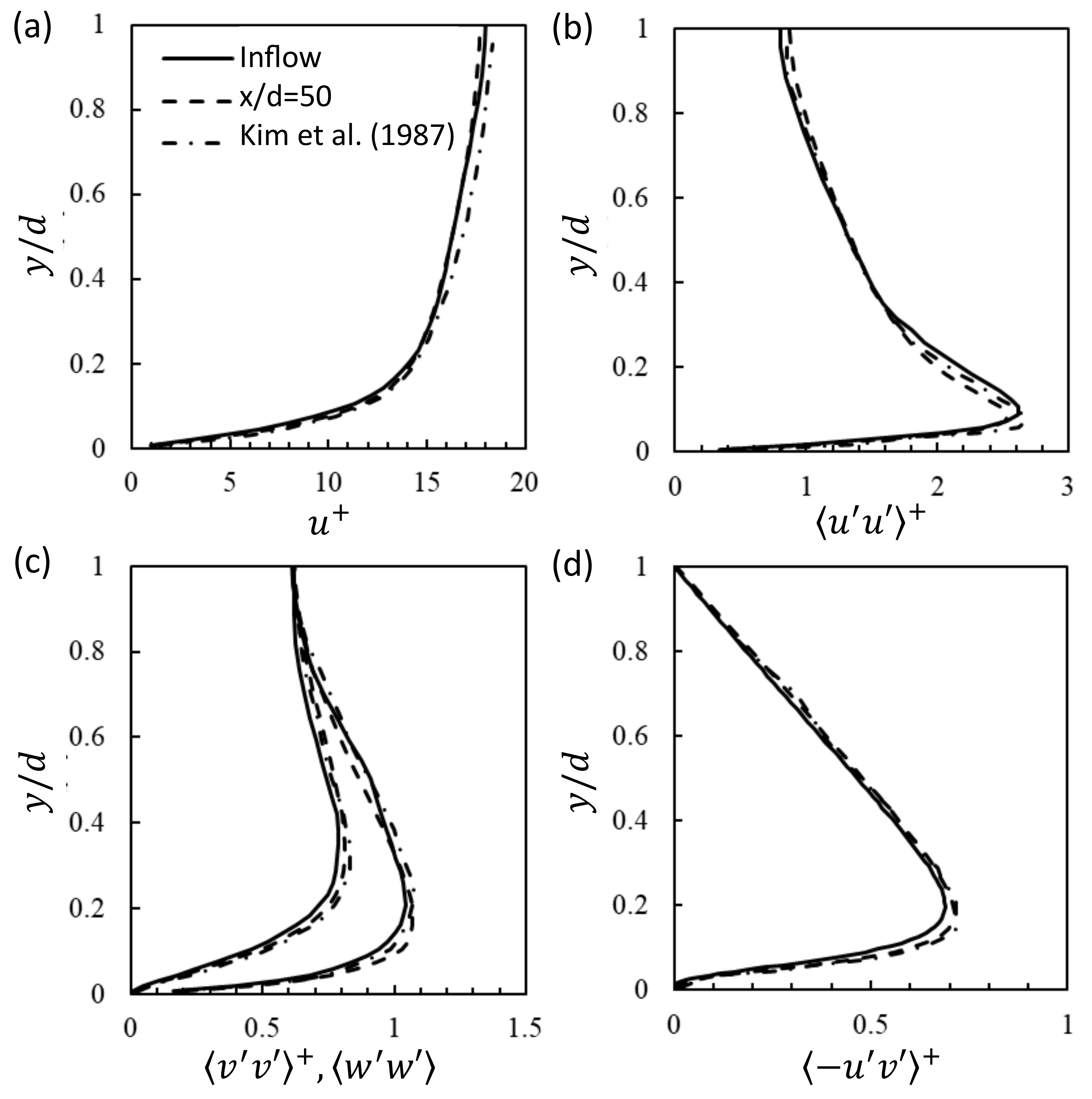
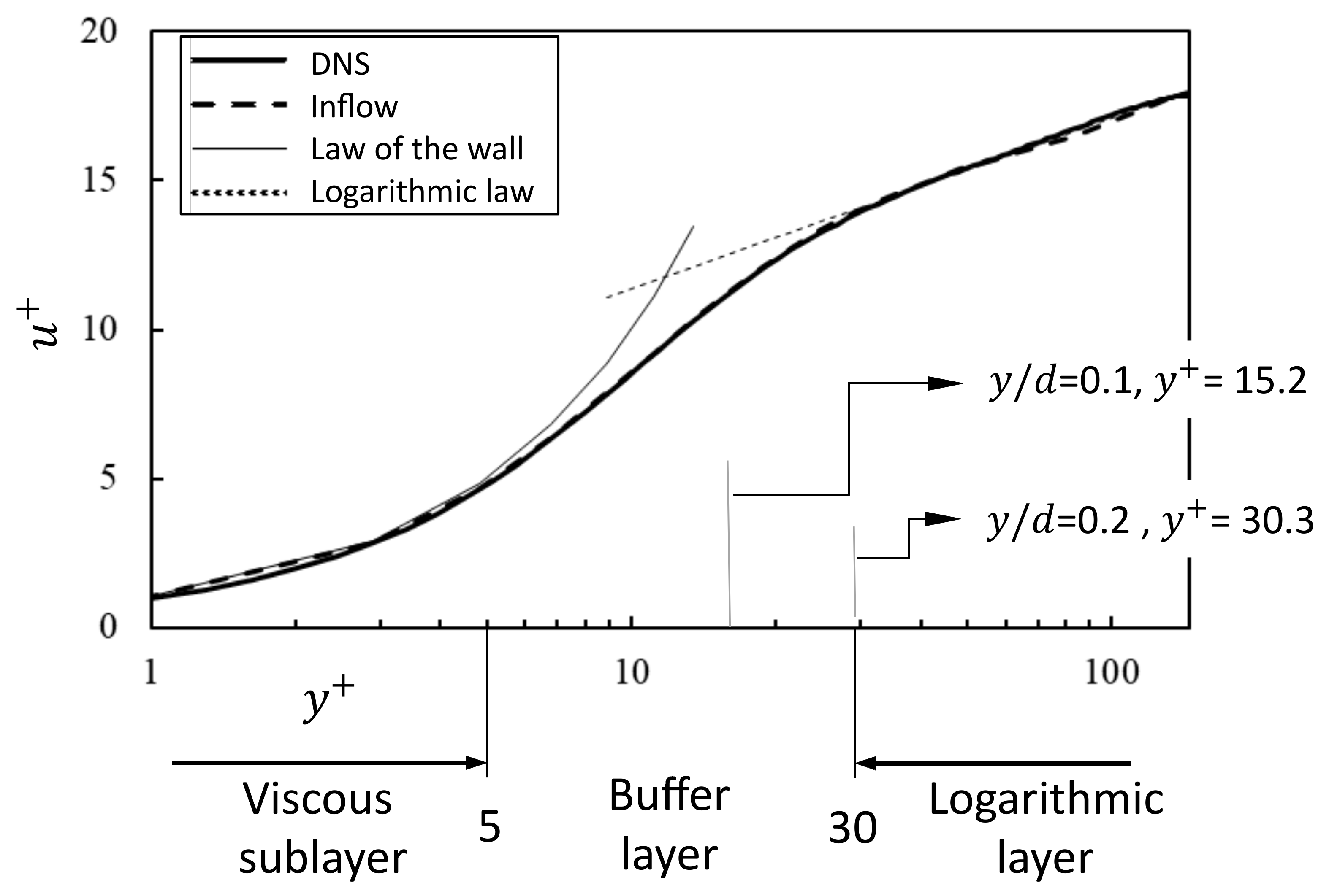
3.1. Channel Flow Simulation Using the Synthetic Inflow Generator

Given that the synthetic inflow generator was available, the channel flow simulation on the LES platform was initially conducted with the aim of observing the development of the turbulent flow in the whole domain. The channel flow started with the data from the synthetic inflow generator, adopting it in the inlet section, and developed the flow downstream to the smooth wall-bounded channel. The development of the axial and shear stress profiles are very important for identifying the fully developed flow, (Kim et al. [37], Deck et al. [41]), as well as obtaining an appropriate turbulent flow downstream.
Figure 4 shows the development of dimensionless axial and shear stress distributions. Figure 4a indicates the variation in the wall shear stress close to the surface from the inlet to downstream of the channel; the ordinate axis indicates the non-dimensional wall shear stress, defined as τ w + = τ w / ( ρ u τ 2 ) , and the abscissa represents the streamwise distance (x) from the inlet normalized by the half height (d) of the channel. To observe the effect of the longitudinal domain size, two different domains ( x / d = 12 and 60) were designed and calculated. As shown in the figure, the wall shear stress decreased near the inlet of the channel and slowly recovered downstream, becoming almost constant at around x / d = 30 (see solid line). Moreover, the short domain case ( x / d = 12 ) did not recover (see dashed line), and the difference between the highest and lowest magnitudes of τ w + was much larger than that of the domain size x / d = 60 . Therefore, if the domain size was set to be less than x / d = 30 , the wall shear stresses would be very low. Figure 4b shows the Reynolds stress profiles at several equi-spaced positions, x / d = 0, 10, 20, 30, 40, and 50, and the abscissa indicates the wall-normal distance from the wall surface normalized by d.
Figure 4c–e indicates the variation of axial stress profiles along the whole domain. Note here that the solid lines in the figure represent the existing DNS data. The axial (longitudinal) stress profiles began initially with the data from the synthetic inflow generator; however, they gradually developed and reached the fully developed profile downstream, which corresponded to the existing DNS data. The vertical and spanwise stress profiles were also not properly developed upstream, but they almost fully developed downstream.
Figure 5 shows the gradient of the dimensionless shear stress, < τ w > + / Δ x , in the streamwise direction with the aim of identifying more precisely the critical point indicating a fully developed boundary layer. As shown in Figure 5, there was a steep gradient near the inlet, and the values < τ w > + / Δ x gradually recovered and converged to an almost constant value (i.e., around zero) in the region where x / d 40 .
Figure 6 shows the mean and turbulent statistics in the channel flow and compares them with the existing DNS data (Kim et al. [42]). In the figure, the fully developed profile was obtained at x / d = 50 , and the inlet data from the inflow generator and the DNS results for the reference and existing data were also compared. As shown in the figure, most of the profiles agreed perfectly well with each other, which was very satisfactory. The turbulent statistics for both cases, that is the inlet and x / d = 50 , also showed a similar pattern. In particular, the non-dimensional mean velocity, u + , was almost identical. The axial longitudinal stress profile, u u + at x / d = 50 also showed a similar distribution near the wall surface compared to that at the inlet. However, when y/d was between 0.1 and 0.4, it was relatively lower than that at the inlet, whereas it was relatively high for y / d between 0.4 and 1.0. The axial vertical stress profile, v v + , and the shear stress, u v + , at x / d = 50 were slightly overestimated compared to the data at the inlet. The difference between the turbulent boundary layers at the inlet and x / d = 50 was due to a relatively coarse resolution of the LES in the core region.

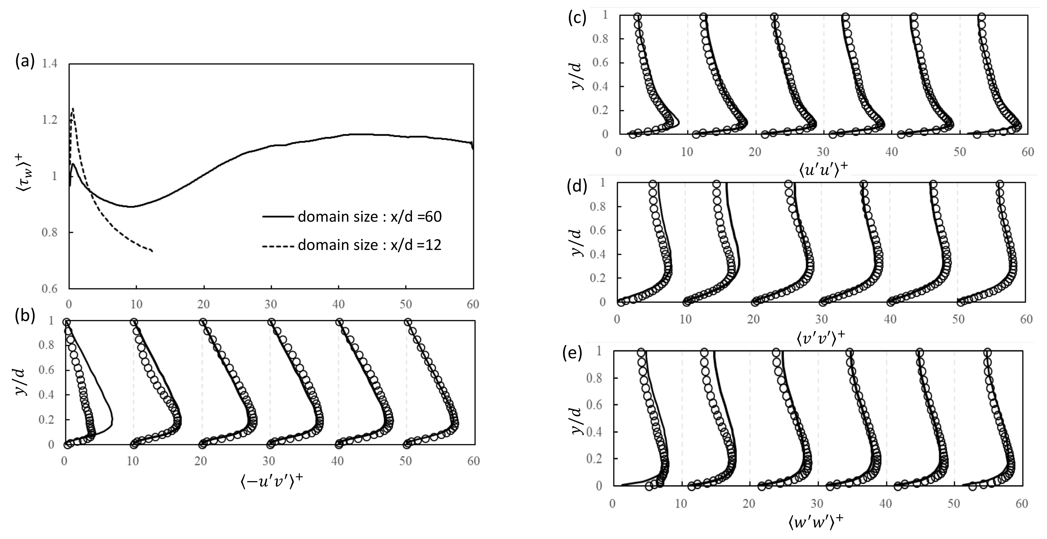
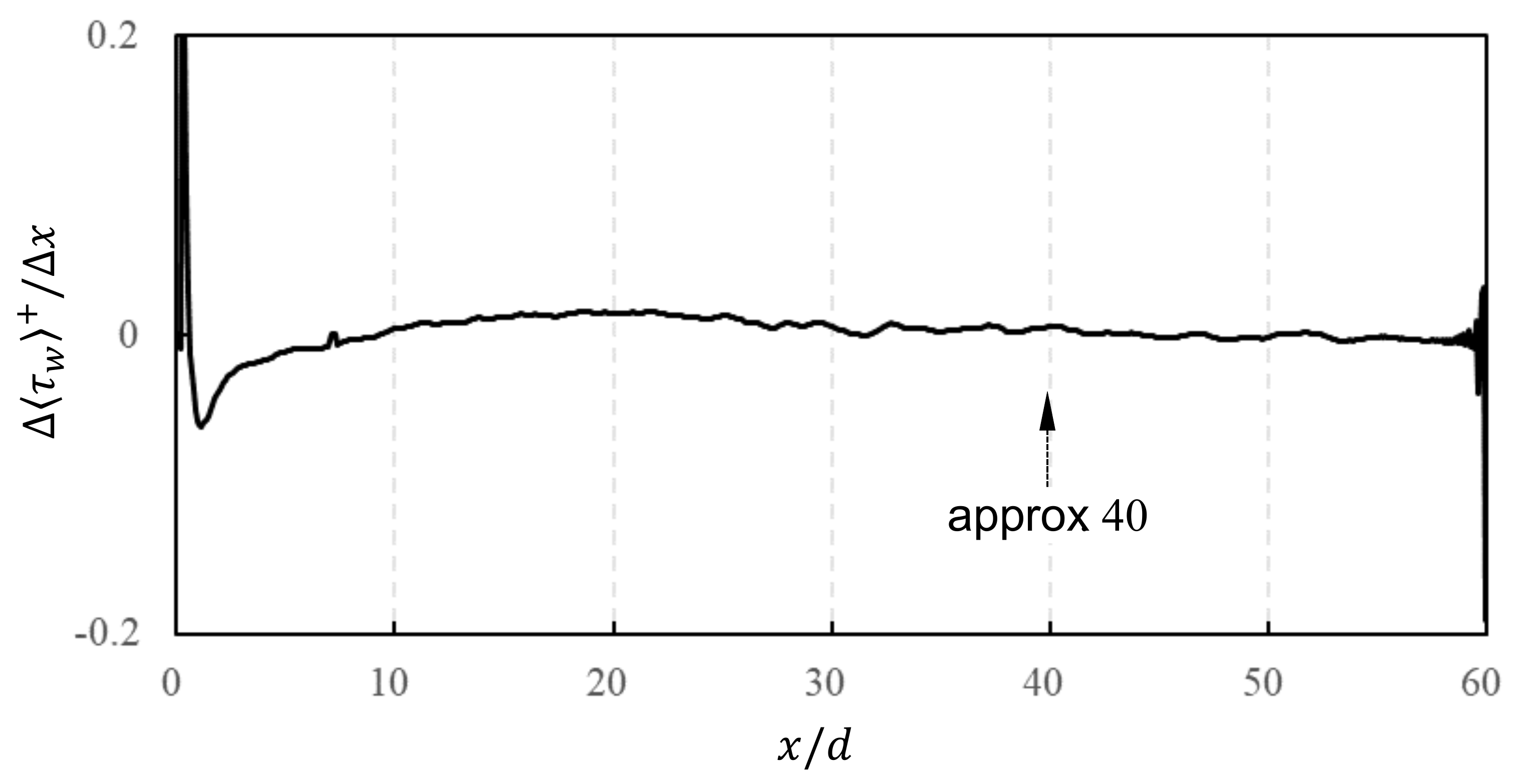
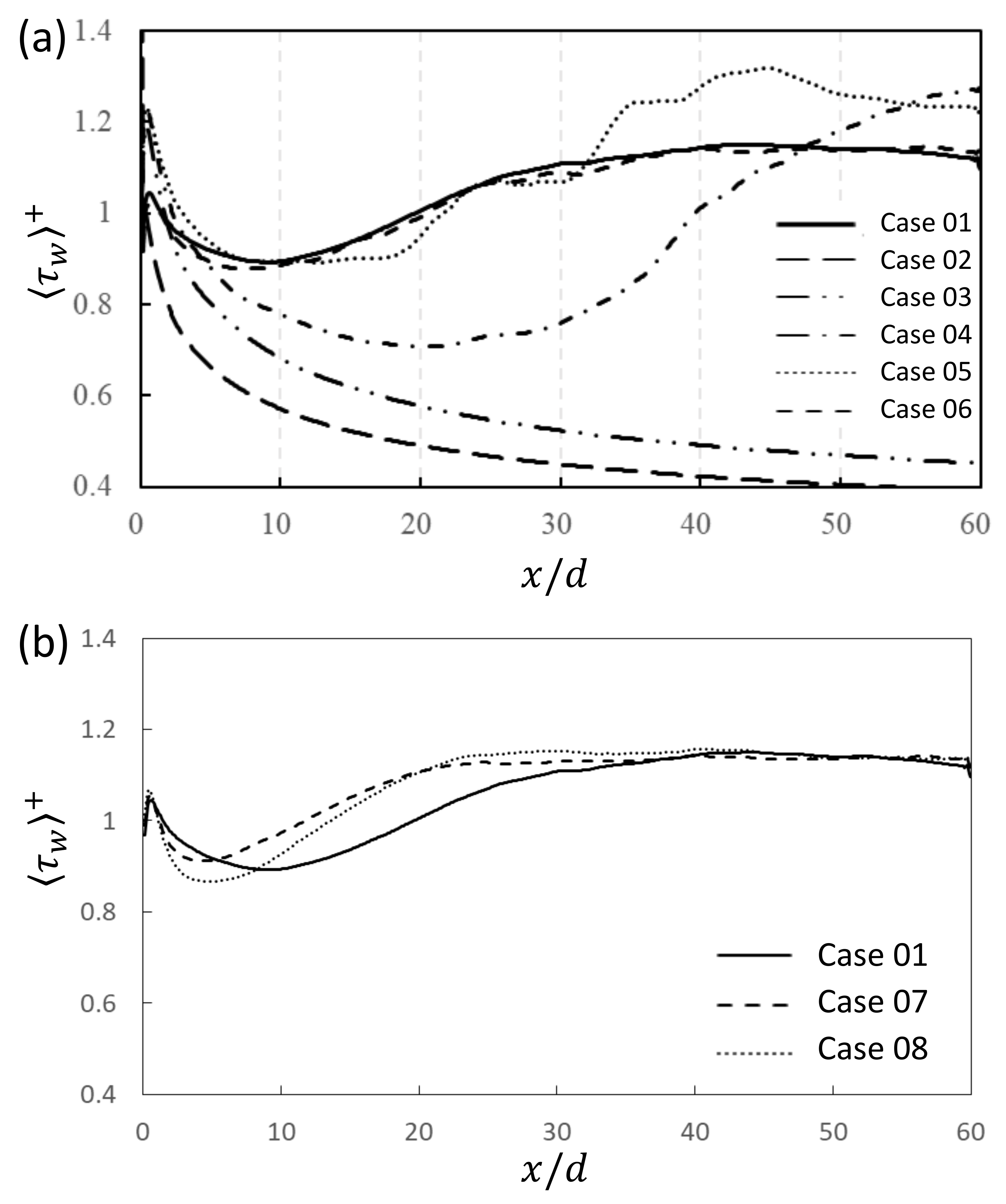
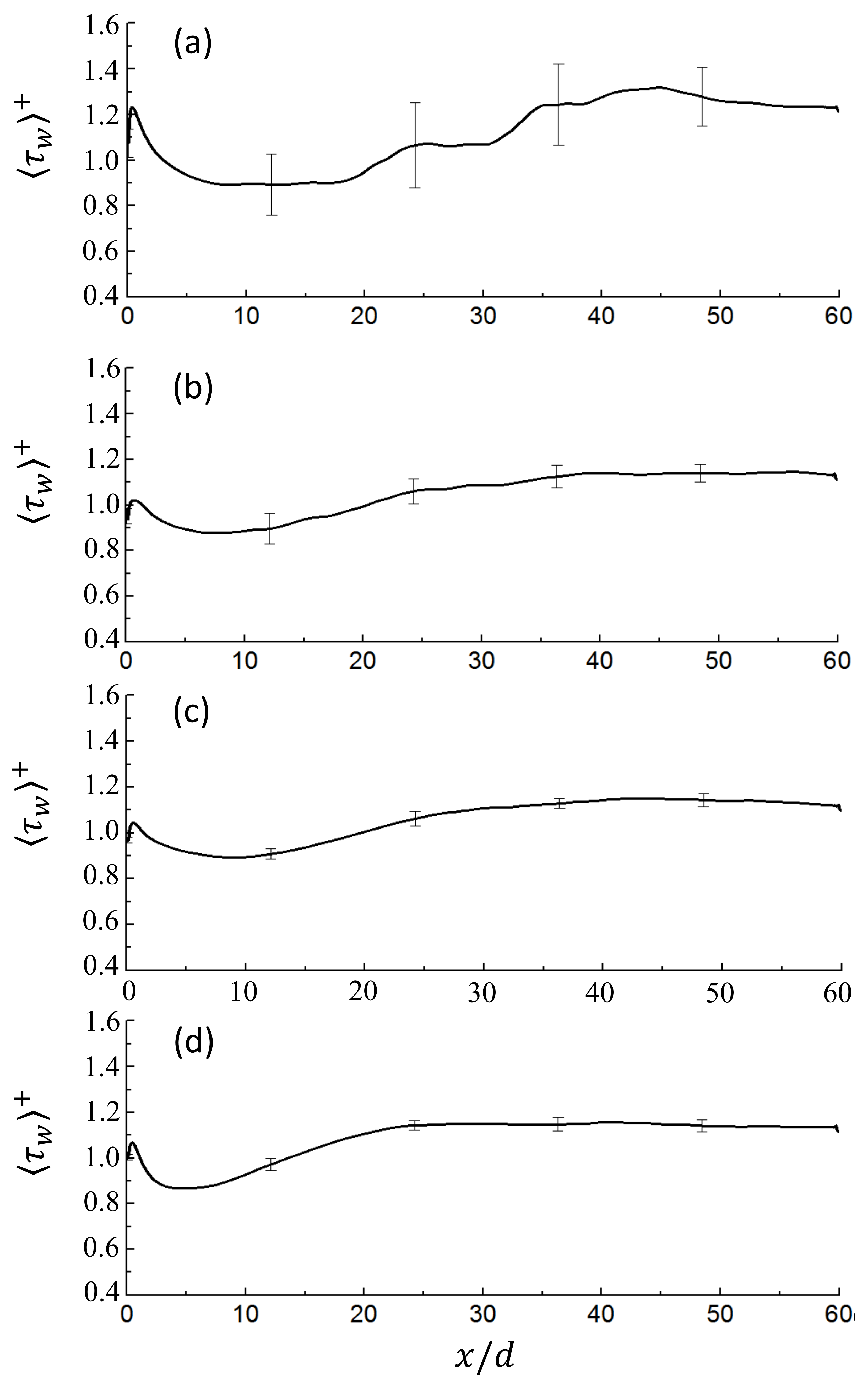
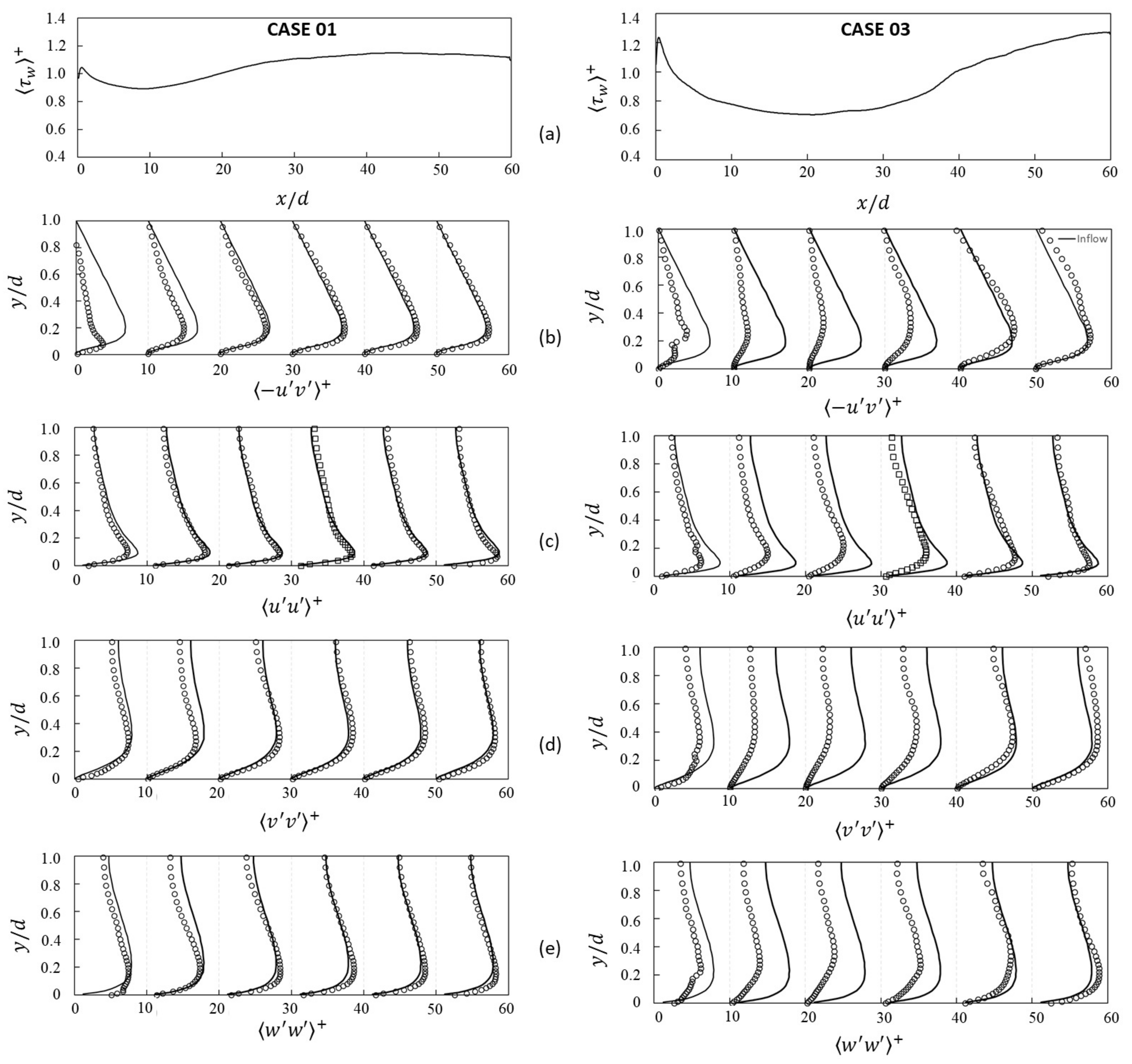
3.2. Effect of Inlet Length Scale on Wall Shear Stress

Figure 7 shows the distribution of the non-dimensional wall shear stress < τ w > + for all the cases of different inlet length scales. Notably, the streamwise length scales were the same for all those cases. To observe the effect of the length scale close to the wall, the spanwise length scale was set from a minimum of 0.15 L z * to a maximum of 3 L z * . It should be noted that the variation in the inlet length scale had a significant effect on the recovery of the wall shear stress downstream. As shown in Figure 7a, Case 01 revealed that the wall shear stress recovered fairly well at x / d = 40 . The wall shear in other cases having a relatively smaller length scale than that in Case 01 was mostly unstable and did not properly recover downstream, except in Case 06.
In Case 02, which was the worst case having no length scale implemented in the inflow, the wall shear stress continuously decreased downstream, and the wall shear stress substantially dropped to approximately 50 % at the outlet compared to that at the inlet. Case 03, in which the length scale was 0.15 L z * , was used in the range y / d < 0.2 , and was shown to be similar to Case 02, although it was slightly larger in terms of shear stress. This was similar to the case having a short domain size of x / d = 12 shown in Figure 4a, which implies that the domain needed to be at least longer than this size in the streamwise direction to obtain fully developed turbulent statistics.
Case 04, which had a smaller length scale (i.e., 0.3 L z * ) in the range y / d < 0.2 , indicated that the shear stress had a local minimum turning point under this condition, and this meant that the shear stress decreased and gradually recovered at a specific point around x / d = 20 . However, the shear stress continued to increase and finally became unstable at a point approximately 14 % higher than that of Case 01. For Case 05, in which the length scale was slightly smaller (i.e., 0.5 L z * ) in the range y / d < 0.2 , but larger (i.e., 1.5 L z * ) for the rest of the range, the wall shear stress appeared to be quite close to that of Case 01 in the inlet region; however, it appeared scattered, wavy, and unstable downstream. Apart from Case 04, it did not tend to continue increasing continuously near the outlet, but it reached a value that was 10 % higher than that in Case 01. In this study, we tried to adjust the size of the length scale in certain zones, such as 0.3 L z * in L z * and L z * in y / d > 0.1 , with the aim of understanding the effect of zone height on flow development. Interestingly, we found that the shear stress agreed fairly well with that in Case 01. This implies that depending on how the length scales were imposed in the zones, the wall shear stress would be adjusted in a target shape inside the domain.
Figure 7b shows the wall shear stress distribution for the cases with a larger inlet length scale (approximately two and/or three times) than that of Case 01 (i.e., L z * ). Interestingly, Cases 07 and 08 (i.e., 2 L z * and 3 L z * ) showed a faster recovery of the wall shear stress compared with Case 01. As shown in the figure, Case 08 had a higher length scale than Case 07, but the distance required to recover in the shear stress would be almost the same, whereas the earlier drop in the shear stress close to the inlet in Case 08 was steeper than that in Case 07.
In the case of the shear stress distribution of Case 01, Case 04, and Case 06 (see Figure 7), these three cases had the same spanwise length scale of 1 L z * at y / d > 0.2 , but the conditions differed at y / d < 0.2 . As shown in the figure, Cases 01 and 06 had very similar shear stress distributions, whereas Case 04 exhibited a markedly different tendency. The difference among these three cases was that the region with 0.3 L z * existed at y / d < 0.2 for Case 04 and at y / d < 0.1 for Case 06. It can be observed that the change in the spanwise length scale in the range 0.1 < y / d < 0.2 had a significant influence on the development of the turbulent boundary layer.
Figure 8 shows the averaged turbulent boundary layer profile, and y / d = 0.1 , 0.2 corresponds to y + = 15.2 , 30.3 , respectively, i.e., y / d = 0.1 was placed in the buffer layer and y / d = 0.2 in the logarithmic layer. With respect to the turbulence characteristics near the wall, some studies (Kline et al. [3], Hinze [43], Grass [44]) reported that the region close to the wall has a highly active turbulence movement, which is associated with the behavior of low-speed streaks and horizontal shear stress in the spanwise direction. In addition, there was a breakup in the region 10 < y + < 30 , which is called “bursting”, contributing as much as 70 % of the turbulence. Kasagi et al. [45] and Smith and Schwartz [46] identified counter-rotating streamwise vortices in the region 14 y + 25 , which contained the most energetic vortices.
According to existing research, the 10 < y + < 30 region contributed greatly to the generation of turbulence. As shown in Figure 7, Cases 01 and 06 had the spanwise length scale of 1 L z * , which was a relatively large scale in 15 < y + < 30 , whereas Case 04 had 0.3 L z * , which means that it had a lower length scale in this region, which was insufficient to generate turbulence statistics. In addition, the lower length scale reduced the energy production such that the minimum distance to recover the shear stress close to the wall was longer. It can be seen here that the change in the length scale in the region y + < 15 did not significantly impact the recovery of the shear stress. Therefore, the results of Case 01 and Case 06 were very similar. The change in the length scale in the approximate region of 15 (0.1) < y + ( y / d ) < 30 (0.2) contributed significantly to the generation of turbulent energy near the wall surface.
Figure 9 shows the streamwise development of the wall shear stress < τ w > + in the domain with the deviation, which indicates the magnitude of data variability as error bars. As the length scale near the wall became smaller (Case 05), the deviation became larger. Interestingly, as shown in the figure, Cases 01 and 06 were very close to each other, whereas the shear stress deviation of Case 06 was relatively large. In this case, the only difference was that Case 06 had a length scale of 0.3 L z * in the region y / d < 0.1 (i.e., y + < 15 ). Therefore, if the spanwise length scale was small, the spatial correlation between two different points became lower such that this case required a relatively long longitudinal length and time to fully develop in the domain. As the length scale increased, the wall shear stress tended to recover quickly. However, when the length scale was 2 L z * or more, the distance required for the full development of the boundary layer did not change significantly.
Figure 10a shows the change in the wall shear stress in the channel domain. In particular, Figure 10b–e shows the distribution of Reynolds stress profiles, u u + , v v + , w w + at each longitudinal position of x / d . As depicted in the figure, Case 01 revealed that the downstream region had fully recovered the shear stress; however, Case 03 had a poor distribution in the domain. This implies that the size of the inlet length scale close to the wall greatly influenced the development of the shear stress. In addition, if the wall shear stress was fully recovered, the axial stresses u u + , v v + , w w + remained constant in the whole domain.
Figure 11 compares the turbulent statistics in the boundary layer flow obtained downstream, at x / d = 50 , from Case 01, Case 06, Case 07, and Case 08 with the data from the synthetic inflow generator in the inlet. As shown in the figure, the turbulent statistics at the inlet and downstream at x / d = 50 clearly had a similar tendency. In Figure 11a, the axial longitudinal stress u u + at x / d = 50 appeared similar near the wall surface compared to the inlet. However, when y / d was between 0.1 and 0.4, it was relatively lower than that of the inlet, and in the range 0.4 to 1.0, u u + was relatively high. For x / d = 50 , all cases had a similar u u + distribution. In Figure 11b–d, the vertical v v + and spanwise w w + components of the axial and shear stresses, u v + at x / d = 50 were all slightly over-estimated compared to that at the inlet. When x / d = 50 , it can be seen that the case having a larger inlet length scale had slightly lower stresses, except for u u + . This appeared to be caused by the fact that the LES resolution was lower than that of DNS.

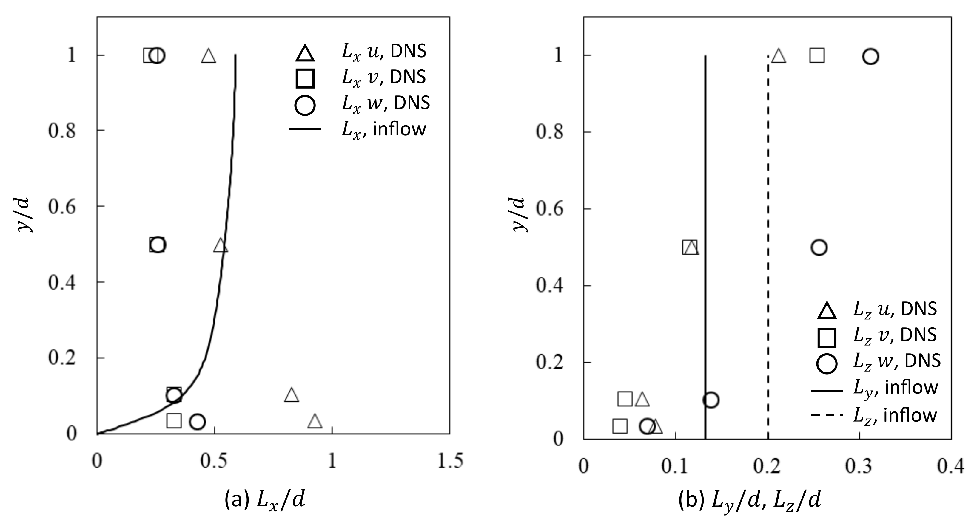
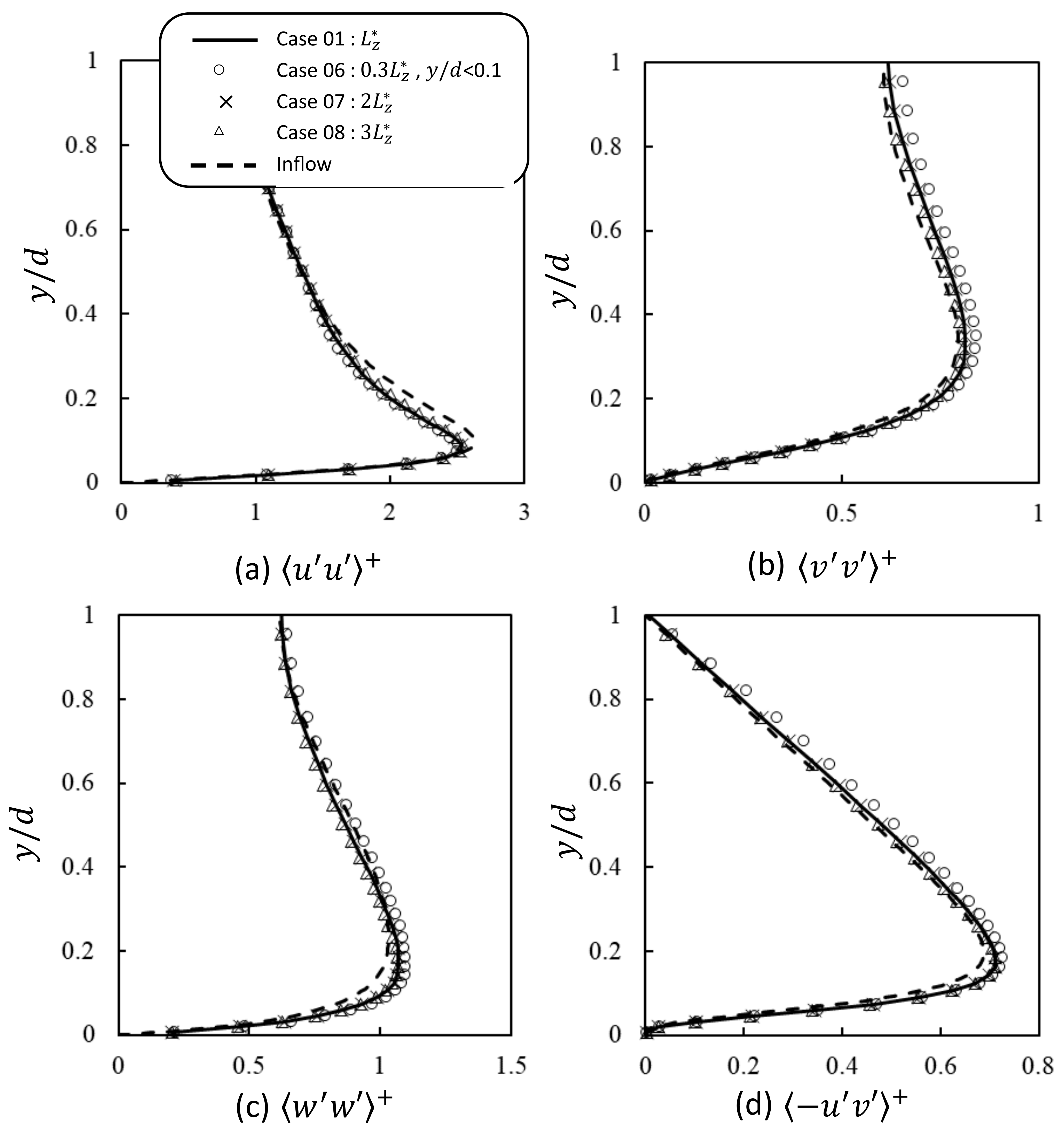
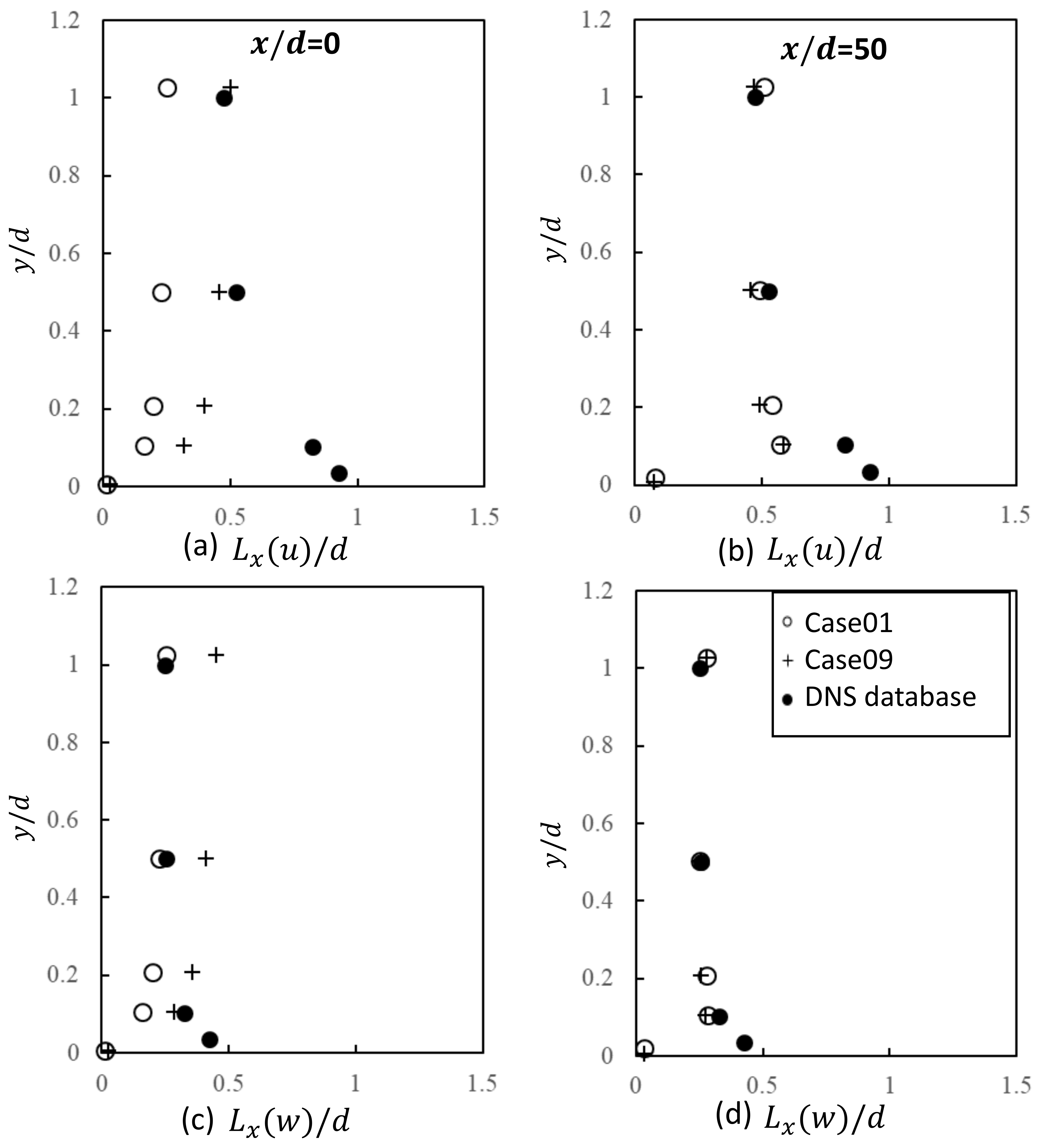
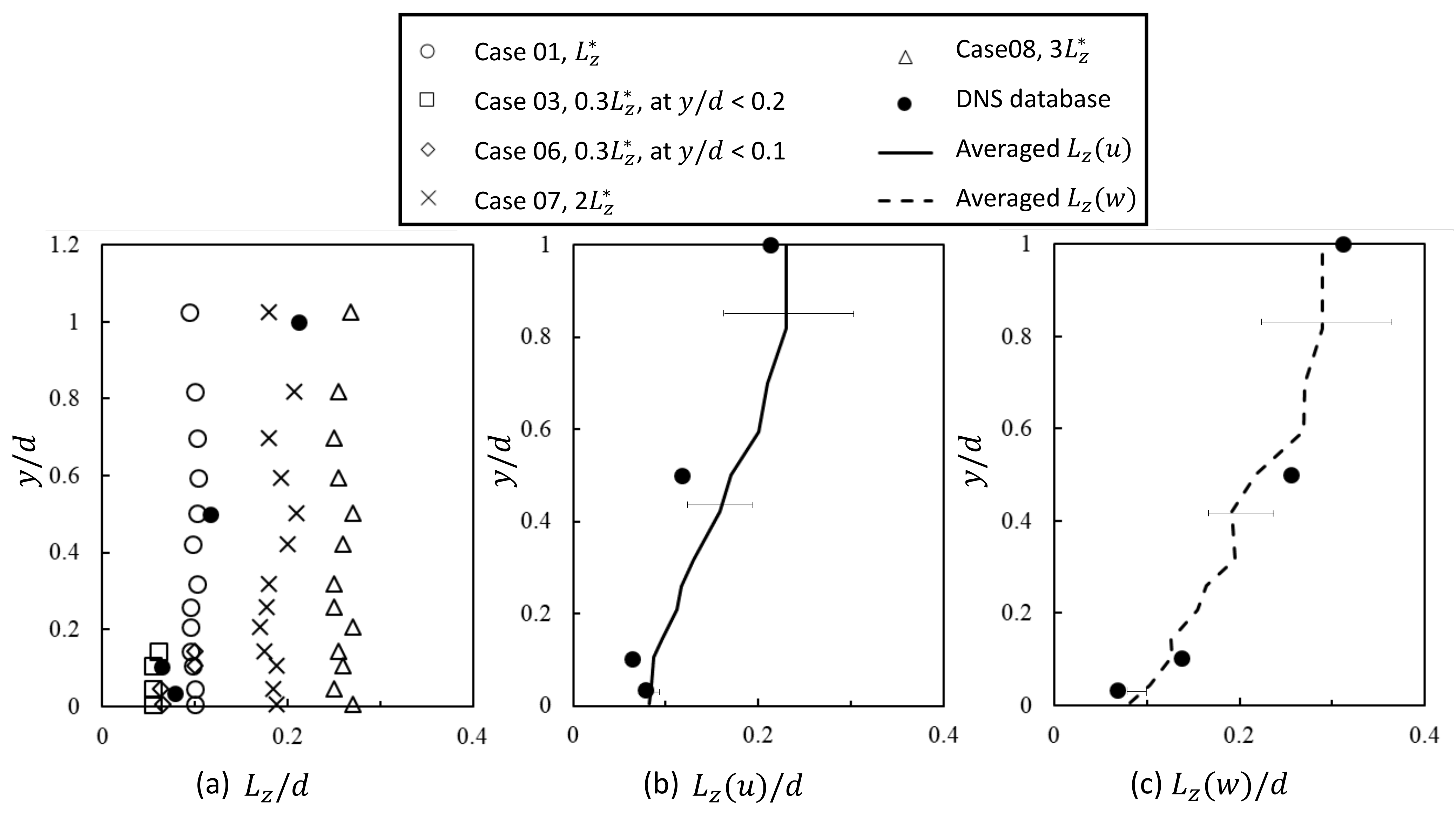
3.3. Effect of Inlet Length Scale on the Integral Length Scale in the Domain

Figure 12 shows the longitudinal integral length scale of the streamwise and vertical velocity (i.e., L x ( u ) and L x ( w ) ) at the inlet section (Figure 12a,c) and at x / d = 50 (Figure 12b,d). As shown in Figure 12a,c, in the cases close to the inlet, the magnitude of the integral length scale L x ( u ) / d close to the wall surface presented a large discrepancy when compared with existing DNS data. On the contrary, the length scales away from the wall (i.e., y / d > 0.5 ) were more similar. In particular, Case 09 (i.e., the case having the largest integral length scale at the inlet) had values very similar to the existing DNS data. The discrepancy between the length scales close to the wall may be due to the fact that the streamwise length scale obtained from the actual DNS was for the fully developed profile; therefore, it was higher than that of the current study close to the wall and gradually decreased in the freestream. Interestingly, even though the length scale was different at the inlet (see Case 02 having no integral length scale at the inlet), the boundary layer developed, and the integral length scale profiles were almost equivalent downstream. This region was fully developed, except for regions that were proximal to the wall. As shown in Figure 12a,c, the longitudinal integral length scale of the vertical velocity (i.e., L x ( w ) ) at the inlet section would have the same tendency as the length scale of the streamwise velocity (i.e., L x ( u ) ).
Figure 13 shows the lateral integral length scale of the streamwise and vertical velocity (i.e., L z ( u ) and L z ( w ) ) at the inlet section (Figure 13) and at x / d = 50 (Figure 13b,c). As mentioned earlier, regardless of the integral length scale at the inlet, the profiles observed downstream were similar, that is they were fully developed.

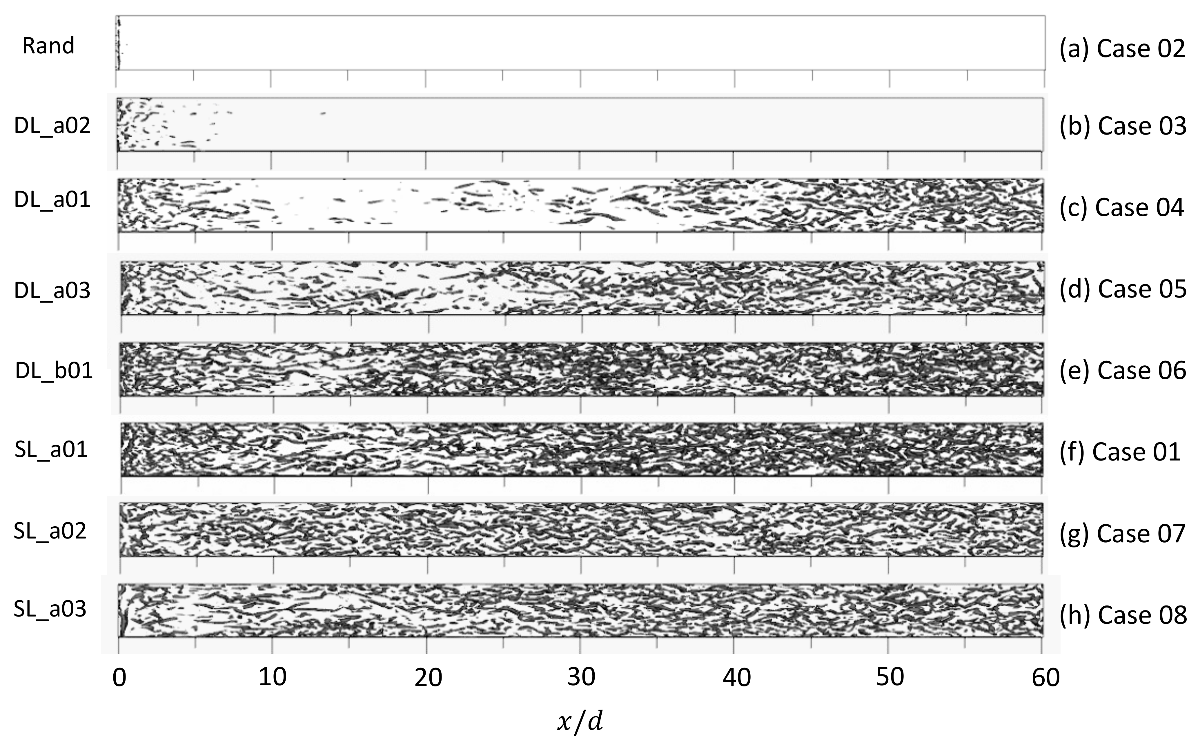
3.4. Second Invariant Flow Structure near the Wall

A second invariant of the velocity gradient tensor can be used to visualize the flow structure near the wall. The related Q-criterion is defined as follows:
Q = 1 2 Ω i j Ω i j S i j S i j
where Ω i j = 1 2 u i x j u j x i and S i j = 1 2 u i x j + u j x i . Ω i j denotes the rotation rate, and S i j denotes the rate of the strain. From the equation, when Q is positive, it means that the intensity of the rotation rate is higher than the deformation rate.
Figure 14 shows the iso-surface of the Q-criterion in the range y / d < 0.25 near the wall. The Q distribution showed a remarkably similar tendency to that of the wall shear stress τ w + distribution in Figure 7. In fact, Case 03, as shown in Figure 7, tended to have a continuous reduction in the shear stress τ w + from the inlet to x / d < 5 , and this was also similar in the Q distribution. In Case 04, as shown in Figure 14b, the Q structure was not observed in the region of 1 < x / d < 35 . This means that when the shear stress was lower than 0.8, the vorticity strength was weak and therefore not enough to form the vortex. Thus, the vortex did not form. In addition, as the shear stress recovered, the vortex reformed when the shear stress was higher than 0.8.
In Figure 14d, that is, in Case 05 and the cases having a length scale higher than 0.5 near the wall, the shear stress was higher than 0.8 in the entire region, and the vortex appeared in the whole area. The vortex structure showed a slight discrepancy depending on the shear stress and the size of the length scale. Interestingly, in the region where the boundary layer was fully developed, the Q structures in all cases (Case 01, Case 07, Case 08) were similar.
Figure 15 shows the energy spectrum distribution at the inlet and for y / d = 50 compared to the existing DNS data. Figure 15a,b includes the results of (c) Case 01 and (d) Case 09. As mentioned earlier, Case 09 had length scales that were two times larger in the streamwise and spanwise directions compared with those of Case 01. In the figure, the symbol k is the wave number, which is defined as 2 π f / U m . Figure 15a,c shows that the energy spectrum at the inlet had an appropriate level at the low wave number region; however, in the higher wave number region, it did not agree with the DNS data. In the figure, the dashed line has a slope of -5/3 in the spectrum. Regardless of the integral length scale at the inlet, the energy spectrum in the fully developed region agreed well with the DNS data.

4. Conclusions

To generate the turbulent boundary layer flow in a numerical domain, a synthetic inflow generator was applied. It was based on spatial and temporal correlation functions, which had the form of an exponential function. To validate the turbulent boundary layer profiles that were obtained by using the synthetic inflow generator, the results obtained were precisely compared with existing data. From the results, it can be concluded that the turbulent boundary layer was successfully generated. In the mean velocity profile u + , the boundary layer agreed well with the overall range of the domain, and the axial and shear stresses were in good agreement with the DNS data.
To observe the effect of the inflow length scales imposed at the inlet section on the development of a turbulent boundary layer, the length scales were varied with a focus on studying their effect. The results showed that a larger length scale in the inlet section had a faster rate of recovery in terms of the wall shear stress, which implies that larger length scales in the inlet section would be essential to the rapid development of the boundary layer, and thereby the realization of a fully developed turbulent boundary layer.
In addition to the variation of the inlet length scale, the inlet plane was separated into two different zones with the aim of imposing two or three different length scales on each zone. The proximity of the wall was chosen to be approximately y / h = 0.1 and 0.2 so that the two ranges were first 0 < y + < 15 (in the middle of the buffer layer zone) and 15 < y + < 150 and, secondly, 0 < y + < 30 (in the buffer layer zone) and 30 < y + < 150 . Based on the results obtained, it can be seen that the length scale variation in the region y + < 15 did not significantly impact the recovery of the wall shear stress. However, the size of the length scale in the region of approximately 15 < y + < 30 contributed significantly to the generation of turbulent energy near the wall surface.

Author Contributions

Conceptualization, Y.-T.L. and H.-C.L.; methodology, Y.-T.L. and H.-C.L.; software, Y.-T.L. and L.K.G.; validation, Y.-T.L. and H.-C.L.; formal analysis, Y.-T.L. and H.-C.L.; investigation, Y.-T.L.; data curation, Y.-T.L.; writing—original draft preparation, Y.-T.L.; writing—review and editing, Y.-T.L. and L.K.G.; supervision, H.-C.L.; project administration, Y.-T.L. and H.-C.L.; funding acquisition, Y.-T.L. and H.-C.L. All authors have read and agreed to the published version of the manuscript.

Funding

This work was funded by the Korea Meteorological Administration Research and Development Program “The Standard Weather Observation and its Application” under Grant (KMA2018-00221). This work was supported by ‘Human Resources Program in Energy Technology’ of the Korea Institute of Energy Technology Evaluation and Planning (KETEP), granted financial resource from the Ministry of Trade, Industry & Energy, Republic of Korea (No. 20214000000140). In addition, this work was supported by the National Research Foundation of Korea (NRF) grant funded by the Korea government (MSIP) (No. 2019R1I1A3A01058576).

Conflicts of Interest

The authors declare that there are no conflicts of interest with respect to the authorship and publication of this article.

References

  1. Kovasznay, L.S. Turbulent boundary layer. Annu. Rev. Fluid Mech. 1970, 2, 95–112. [Google Scholar] [CrossRef]
  2. Willmarth, W.W. Pressure-fluctuations beneath turbulent boundary-layers. Annu. Rev. Fluid Mech. 1975, 7, 13–38. [Google Scholar] [CrossRef]
  3. Kline, S.J.; Reynolds, W.C.; Schraub, F.A.; Runstadler, P.W. The structure of turbulent boundary-layers. J. Fluid Mech. 1967, 30, 741–773. [Google Scholar] [CrossRef] [Green Version]
  4. Sreenivasan, K.R. The turbulent boundary layer. Front. Exp. Fluid Mech. 1989, 46, 159–210. [Google Scholar]
  5. Kline, S.J.; Robinson, S.K. Quasi-Coherent Structures in the Turbulent Boundary Layer. Part I: Status Report on a Community-Wide Summary of the Data. In Near Wall Turbulence; Hemisphere Publishing Corp: New York, NY, USA, 1990; pp. 200–217. [Google Scholar]
  6. Cermak, J.E.; Cochran, L.S. Physical modeling of the atmospheric surface-layer. J. Wind Eng. Ind. Aero. 1992, 42, 935–946. [Google Scholar] [CrossRef]
  7. Rachele, H.; Tunick, A.; Hansen, F.V. Mariah—A similarity-based method for determining wind, temperature, and humidity profile structure in the atmospheric surface-Layer. J. Appl. Meteorol. 1995, 34, 1000–1005. [Google Scholar] [CrossRef] [Green Version]
  8. Rachele, H.; Tunick, A.; Hansen, F.V. Reply to Arya, S.P. Comments on “Mariah—A similarity-based method for determining wind, temperature, and humidity profile structure in the atmospheric surface”. J. Appl. Meteorol. 1996, 35, 613–614. [Google Scholar] [CrossRef] [Green Version]
  9. Raupach, M.R.; Antonia, R.A.; Rajagopalan, S. Rough-wall turbulent boundary layers. Appl. Mech. Rev. 1991, 44, 1–25. [Google Scholar] [CrossRef]
  10. Meroney, R.N. Wind-tunnel modeling of the flow about bluff-Bodies. J. Wind Eng. Ind. Aero. 1988, 29, 203–223. [Google Scholar] [CrossRef] [Green Version]
  11. Kolmogorov, A.N. The local structure of turbulence in incompressible viscous fluid for very large Reynolds numbers. Cr. Acad. Sci. URSS 1941, 30, 301–305. [Google Scholar]
  12. Prandtl, L. On fluid motions with very small friction. Verhldg 1904, 3, 484–491. [Google Scholar]
  13. Tennekes, H.; Lumley, J.L. A First Course in Turbulence; MIT Press: Cambridge, MA, USA, 1972; 300p. [Google Scholar]
  14. Hunt, A. Wind-tunnel measurements of surface pressures on cubic building models at several scales. J. Wind Eng. Ind. Aero. 1982, 10, 137–163. [Google Scholar] [CrossRef]
  15. Sun, J.; Mahrt, L. Determination of surface fluxes from the surface radiative temperature. J. Atmos. Sci. 1995, 52, 1096–1106. [Google Scholar] [CrossRef] [Green Version]
  16. Lee, S.; Lele, S.K.; Moin, P. Simulation of spatially evolving turbulence and the applicability of Taylor hypothesis in compressible flow. Phys. Fluids 1992, 4, 1521–1530. [Google Scholar] [CrossRef]
  17. Keating, A.; Piomelli, U.; Balaras, E.; Kaltenbach, H. A priori and a posteriori tests of inflow conditions for large-eddy simulation. Phys. Fluids 2004, 16, 4696–4712. [Google Scholar] [CrossRef]
  18. Lim, H.C.; Thomas, T.G.; Castro, I.P. Flow around a cube in a turbulent boundary layer: LES and experiment. J. Wind. Eng. Ind. Aero. 2009, 97, 96–109. [Google Scholar] [CrossRef] [Green Version]
  19. Lim, H.C.; Castro, I.P.; Hoxey, R.P. Bluff bodies in deep turbulent boundary layers: Reynolds-number issues. J. Fluid Mech. 2007, 571, 97–118. [Google Scholar] [CrossRef] [Green Version]
  20. Lund, T.S.; Wu, X.H.; Squires, K.D. Generation of turbulent inflow data for spatially-developing boundary layer simulations. J. Comput. Phys. 1998, 140, 233–258. [Google Scholar] [CrossRef] [Green Version]
  21. Druault, P.; Lardeau, S.; Bonnet, J.P.; Coiffet, F.; Delville, J.; Lamballais, E.; Largeau, J.F.; Perret, L. Generation of three-dimensional turbulent inlet conditions for large-eddy simulation. AIAA J. 2004, 42, 447–456. [Google Scholar] [CrossRef]
  22. Johansson, P.S.; Andersson, H.I. Generation of inflow data for inhomogeneous turbulence. Theor. Comput. Fluid Dyn. 2004, 18, 371–389. [Google Scholar] [CrossRef]
  23. Perret, L.; Delville, J.; Manceau, R.; Bonnet, J.-P. Generation of turbulent inflow conditions for large eddy simulation from stereoscopic PIV measurements. Int. J. Heat Fluid Flow 2006, 27, 576–584. [Google Scholar] [CrossRef]
  24. Hanna, S.R.; Tehranian, S.; Carissimo, B.; Macdonald, R.W.; Lohner, R. Comparisons of model simulations with observations of mean flow and turbulence within simple obstacle arrays. Atmos. Environ. 2002, 36, 5067–5079. [Google Scholar] [CrossRef]
  25. Xie, Z.T.; Castro, I.P. LES and RANS for turbulent flow over arrays of wall-mounted obstacles. Flow Turbul. Combust. 2006, 76, 291–312. [Google Scholar] [CrossRef] [Green Version]
  26. Xie, Z.T.; Castro, I.P. Efficient generation of inflow conditions for large eddy simulation of street-scale flows. Flow Turbul. Combust. 2008, 81, 449–470. [Google Scholar] [CrossRef] [Green Version]
  27. Mare, L.; Klein, M.; Jones, W.P.; Janicka, J. Synthetic turbulence inflow conditions for large-eddy simulation. Phys. Fluids 2006, 18, 025107. [Google Scholar] [CrossRef]
  28. Veloudis, I.; Yang, Z.; McGuirk, J.J.; Page, G.J.; Spencer, A. Novel implementation and assessment of a digital filter based approach for the generation of LES inlet conditions. Flow Turbul. Combust. 2007, 79, 1–24. [Google Scholar] [CrossRef]
  29. Jarrin, N.; Benhamadouche, S.; Laurence, D.; Prosser, R. A synthetic-eddy-method for generating inflow conditions for large-eddy simulations. Int. J. Heat Fluid Flow 2006, 27, 585–593. [Google Scholar] [CrossRef] [Green Version]
  30. Deck, S.; Renard, N.; Laraufie, R.; Sagaut, P. Zonal detached eddy simulation (ZDES) of a spatially developing flat plate turbulent boundary layer over the Reynolds number range 3150 < Reθ < 14,000. Phys. Fluids 2014, 26, 025116. [Google Scholar] [CrossRef]
  31. Gupta, M.M.; Kalita, J.C. A new paradigm for solving Navier-stokes equations, streamfunction-velocity formulation, J. Comput. Phys. 2005, 207, 25–68. [Google Scholar] [CrossRef]
  32. Barragy, E.; Carey, G.F. Stream function-vorticity driven cavity solution using p finite elements. Comput. Fluids 1997, 26, 453–468. [Google Scholar]
  33. Bennacer, R.; Reggio, M.; Pellerin, N.; Ma, X.Y. Differentiated heated lid driven cavity interacting with tube a Lattice Boltzmann Study. Therm. Sci. 2017, 21, 89–104. [Google Scholar]
  34. Kareem, A.K.; Gao, S. Mixed convection heat transfer of turbulent flow in a three-dimensional lid-driven cavity with a rotating cylinder. J. Heat Mass Transf. 2017, 112, 185–200. [Google Scholar] [CrossRef] [Green Version]
  35. Moin, P.; Kim, J. Numerical investigation of turbulent channel flow. J. Fluid Mech. 1982, 118, 341–377. [Google Scholar] [CrossRef] [Green Version]
  36. Le, H.; Moin, P. Direct Numerical Simulation of Turbulent Flow Over a Backward-Facing Step; Standford Univ. Report TF-58; Department of Mechanical Engineering, Cambridge University Press: Cambridge, UK, 1994. [Google Scholar]
  37. Kim, Y.; Castro, I.P.; Xie, Z.T. Divergence-free turbulence inflow conditions for large-eddy simulations with incompressible flow solvers. Comput. Fluids 2013, 84, 56–68. [Google Scholar] [CrossRef] [Green Version]
  38. Solorzano-Lopez, J.; Zenit, R.; Ramirez-Argaez, M.A. Mathematical and physical simulation of the interaction between a gas jet and a liquid free surface. Appl. Math. Model. 2011, 35, 4991–5005. [Google Scholar] [CrossRef]
  39. Taylor, G.I. The spectrum of turbulence. Proc. R. Soc. Lond. Ser. Math. Phys. Sci. 1938, 164, 476–490. [Google Scholar] [CrossRef] [Green Version]
  40. Iwamoto, K.; Suzuki, Y.; Kasagi, N. Database of Fully Developed Channel Flow. Department of Mechanical Engineering, The University of Tokyo, THTLAB Internal Report No. ILR-0201, DNS Database (CH12_PG.WL7). 2002. Available online: http://www.thtlab.jp (accessed on 15 May 2021).
  41. Deck, S.; Weiss, P.E.; Pamies, M.; Garnier, E. Zonal detached eddy simulation of a spatially developing flat plate turbulent boundary layer. Comput. Fluids 2011, 48, 1–15. [Google Scholar] [CrossRef]
  42. Kim, J.; Moin, P.; Moser, R. Turbulence statistics in fully developed channel flow at low Reynolds number. J. Fluid Mech. 1987, 177, 133–166. [Google Scholar] [CrossRef] [Green Version]
  43. Hinze, J. Turbulence; McGraw-Hill: New York, NY, USA, 1975. [Google Scholar]
  44. Grass, A.J. Structural features of turbulent flow over smooth and rough boundaries. J. Fluid Mech. 1971, 50, 233–255. [Google Scholar] [CrossRef]
  45. Kasagi, N.; Hirata, M.; Nishino, K. Streamwise pseudo-vortical structures and associated vorticity in the near-wall region of a wall-bounded turbulent shear flow. Exp. Fluids 1986, 4, 309–318. [Google Scholar] [CrossRef]
  46. Smith, C.; Schwartz, S. Observation of streamwise rotation in the near-wall region of a turbulent boundary layer. Phys. Fluids 1983, 26, 641–652. [Google Scholar] [CrossRef]
Figure 1. Schematic diagram of the computational domain (total number of cells: 600 × 60 × 70 ).
Applsci 11 05177 g001
Figure 2. Integral length scales (symbol: two-point correlation in DNS data; line: inflow generation).
Applsci 11 05177 g002
Figure 3. Statistical profiles from DNS and the synthetic inflow generator. (a) mean velocity profiles (b) streamwise stress profiles (c) vertical and transverse stress profiles (d) Reynolds stress profiles.
Applsci 11 05177 g003
Figure 4. Spatial development of: (a) dimensionless wall shear stress; (b) shear stress; (c) axial stress (longitudinal); (d) axial stress (vertical); (e) axial stress (spanwise).
Applsci 11 05177 g004
Figure 5. Variation of dimensionless wall shear stress per grid size.
Applsci 11 05177 g005
Figure 6. Mean and turbulent statistics in channel flow at the inlet, x / d = 50 , and comparison with the study of Kim et al. [42]. (a) mean velocity profiles (b) streamwise stress profiles (c) vertical and transverse stress profiles (d) Reynolds stress profiles.
Applsci 11 05177 g006
Figure 7. Development of dimensionless wall shear stress with different length scales. (a) Cases 01–06 (b) Cases 01, 07 and 08.
Applsci 11 05177 g007
Figure 8. Mean streamwise velocity profiles. y / d = 0.1 , 0.2 denote y + = 15.2 , 30.3 , respectively.
Applsci 11 05177 g008
Figure 9. Variation of dimensionless wall shear stress and deviation in the domain with changing length scales for (a) Case 05, (b) Case 06, (c) Case 01, and (d) Case 08.
Applsci 11 05177 g009
Figure 10. Development of dimensionless wall shear stress and axial stresses. In the figure, at the left: Case 01, at the right: Case 03, solid line: DNS data, ∘: simulation results. (a) wall shear stress, (b) Reynolds shear stress, (c) streamwise shear stress, (d) transverse shear stress, and (e) vertical shear stress.
Applsci 11 05177 g010
Figure 11. Mean and turbulent stress profiles at x / d = 50 . In the figure, (a) u u + , (b) v v + , (c) w w + , (d) u v + .
Applsci 11 05177 g011
Figure 12. Longitudinal integral length scale profiles at the inlet section (a,c) and at x / d = 50 (b,d), L x ( u ) / d : (a,b), L x ( w ) / d : (a,b). In the figure, (a) denotes longitudinal integral length scales of the streamwise velocity component at inlet section, (b) longitudinal integral length scales of the streamwise velocity component at x / d = 50 , (c) longitudinal integral length scales at the inlet section of the spanwise velocity component, and (d) longitudinal integral length scales of the spanwise velocity component at x / d = 50 , (∘: Case01, +: Case09, •: DNS database).
Applsci 11 05177 g012
Figure 13. Lateral integral length scale distribution at the inlet and downstream sections. In the figure, (a) denotes all the lateral integral length scales at the inlet section (∘: Case01, □: Case03, ⋄: Case06, ×: Case07, Δ: Case08, •: DNS database), (b) the lateral integral length scale of streamwise velocity components at x/d = 50 (•: DNS database, : Averaged L z ( u ) ), and (c) the lateral integral length scale of spanwise velocity components at x / d = 50 (•: DNS database, — — —: averaged L z ( w ) ).
Applsci 11 05177 g013
Figure 14. Iso-surface of the Q-criterion at y / d < 0.25 and the value of Q > 1 .
Applsci 11 05177 g014
Figure 15. Energy spectrum distribution at the inlet (a,c) and for y / d = 50 (b,d). In addition, (a,b) are the results from Case 01 and (c,d) from Case 09.
Applsci 11 05177 g015
Table 1. Size of length scales applied in the simulation.
Name y / d < 0.1 0.1 < y / d < 0.2 y / d > 0.2
Case 01 1 L z * 1 L z * 1 L z *
Case 020, random0, random0, random
Case 03 0.15 L z * 0.15 L z * 0.5 L z *
Case 04 0.3 L z * 0.3 L z * 1 L z *
Case 05 0.5 L z * 0.5 L z * 1.5 L z *
Case 06 0.3 L z * 1 L z * 1 L z *
Case 07 2 L z * 2 L z * 2 L z *
Case 08 3 L z * 3 L z * 3 L z *
Publisher’s Note: MDPI stays neutral with regard to jurisdictional claims in published maps and institutional affiliations.

