
A Hybrid Gearbox Fault Diagnosis Method Based on GWO-VMD and DE-KELM


Abstract
:Featured Application
Abstract
1. Introduction
1.1. Motivations
1.2. State of the Art of Gearbox Fault Diagnosis
1.2.1. Feature Signal Adaptive Processing Aspect
1.2.2. Fault Identification Aspect
1.3. Organization of This Article
2. Common Faults of Gearboxes and Causes Analysis
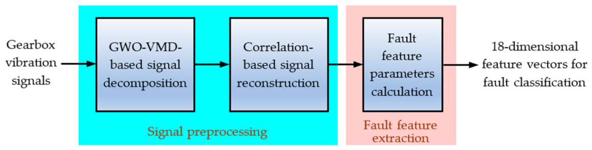
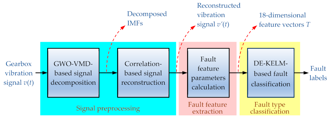
3. Vibration Signal Preprocessing and Fault Feature Extraction
3.1. GWO-VMD-Based Vibration Signal Decomposition
3.1.1. Basic Principle of VMD
3.1.2. Deficiencies of VMD
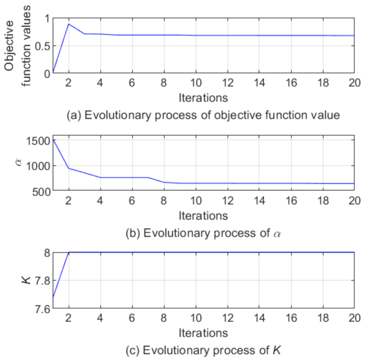
3.1.3. GWO-Based [K, α] Optimization for VMD
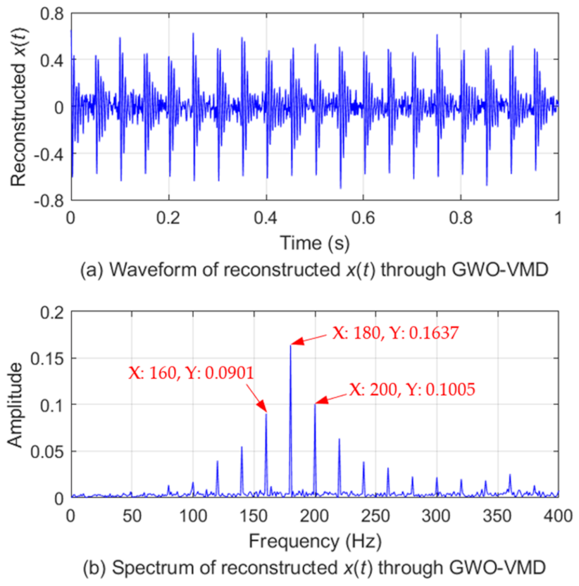
3.2. Correlation-Based Gearbox Vibration Signal Reconstruction
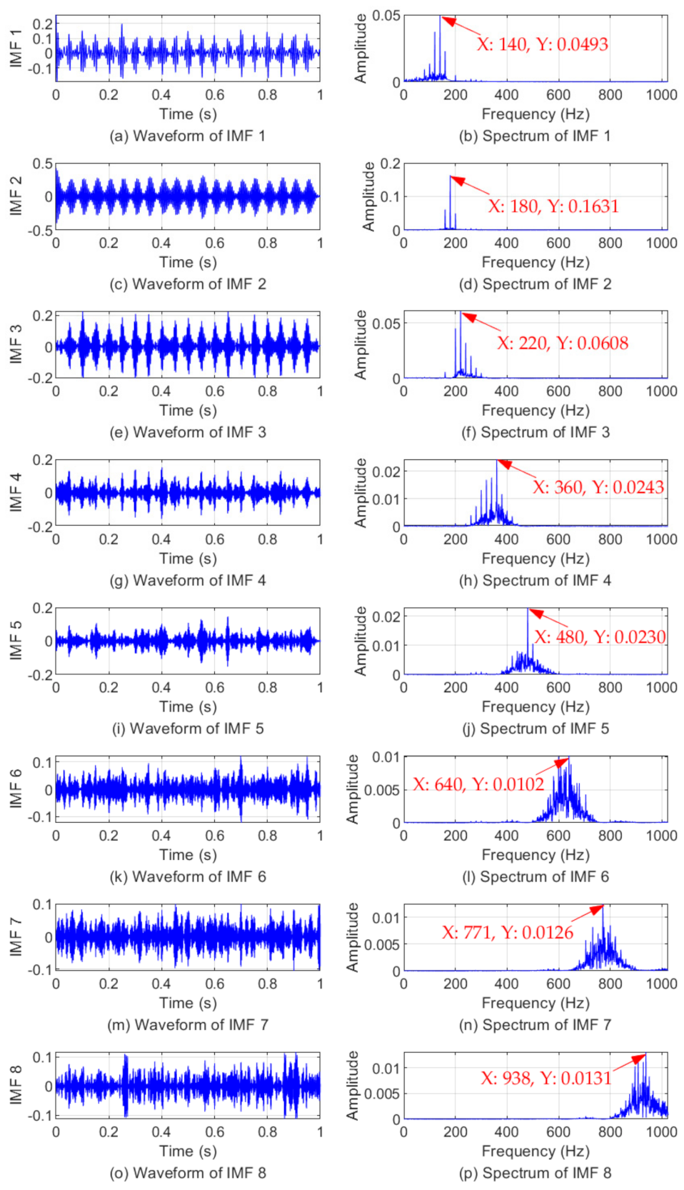
3.3. Fault Feature Extraction
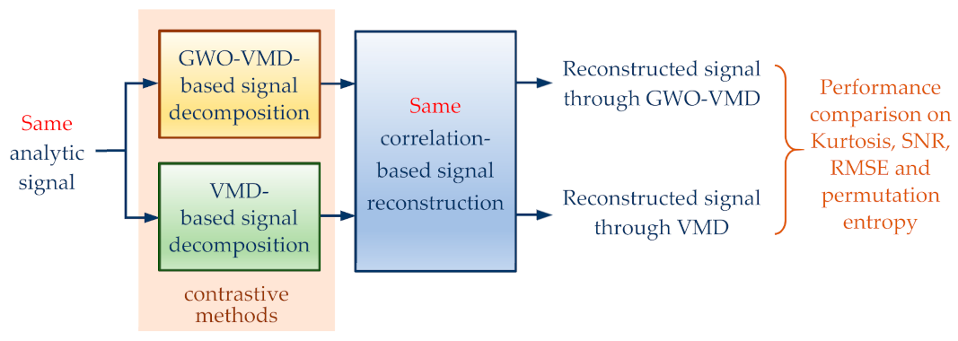
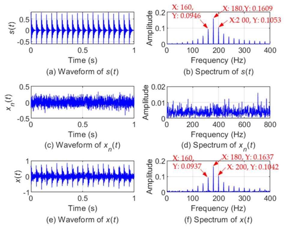
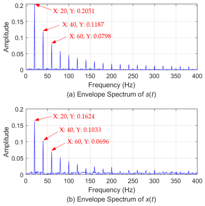
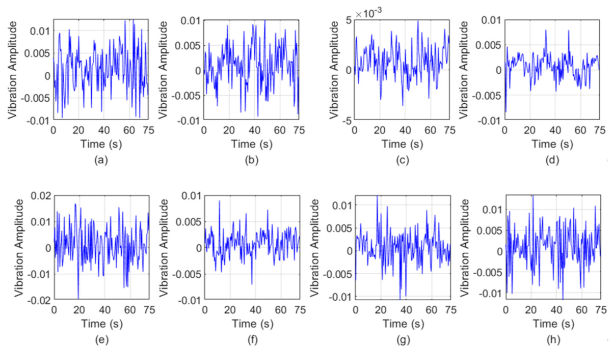
3.4. Method Verification Experiments
4. DE-KELM-Based Gearbox Fault Classification
4.1. Basic Principle of KELM
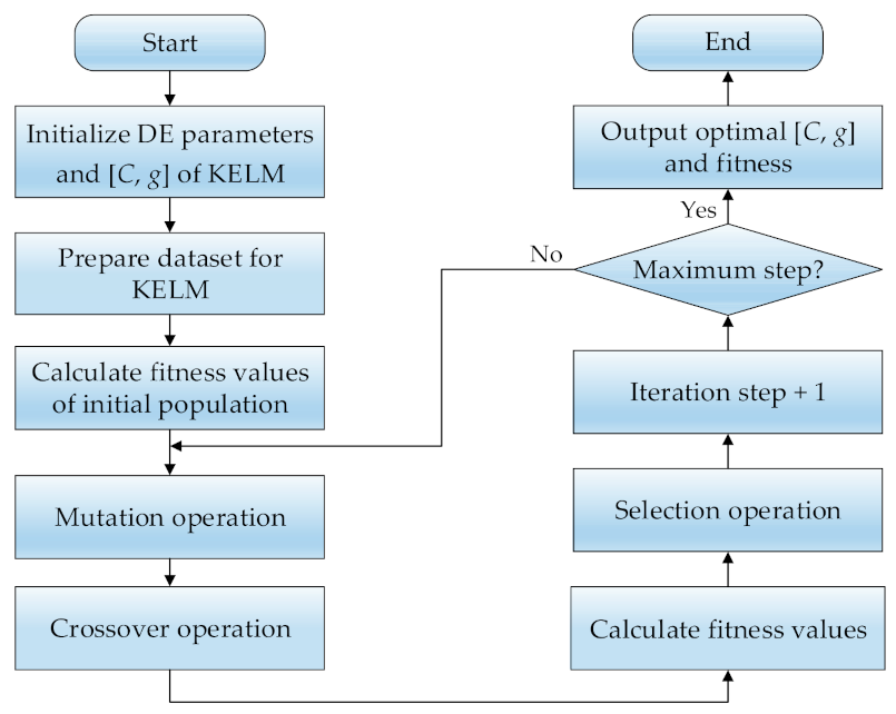
4.2. DE-KELM-Based Fault Classification
4.3. Method Verification Experiments
5. Experimental Validation and Result Analysis
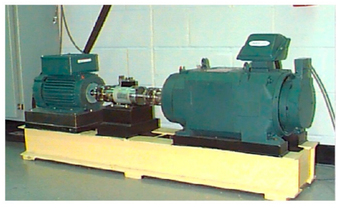
5.1. Gearbox Fault Diagnosis Experimental Data
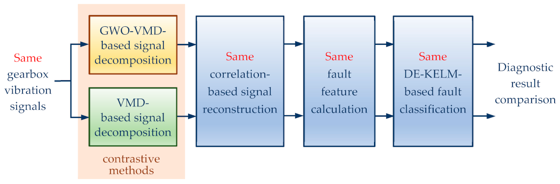
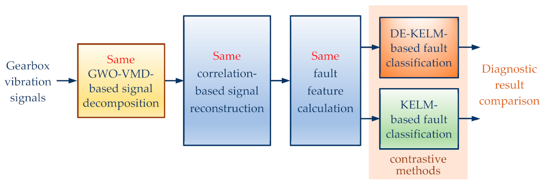
5.2. Contrast Experiment I—Gearbox Fault Diagnosis with Contrasting Vibration Signal Decomposition Methods: GWO-VMD and VMD
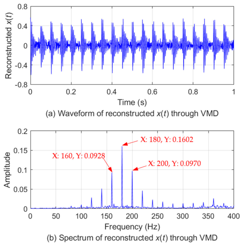
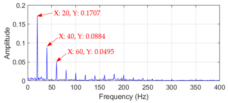
5.2.1. Vibration Signals Decomposition through GWO-VMD and VMD, Respectively
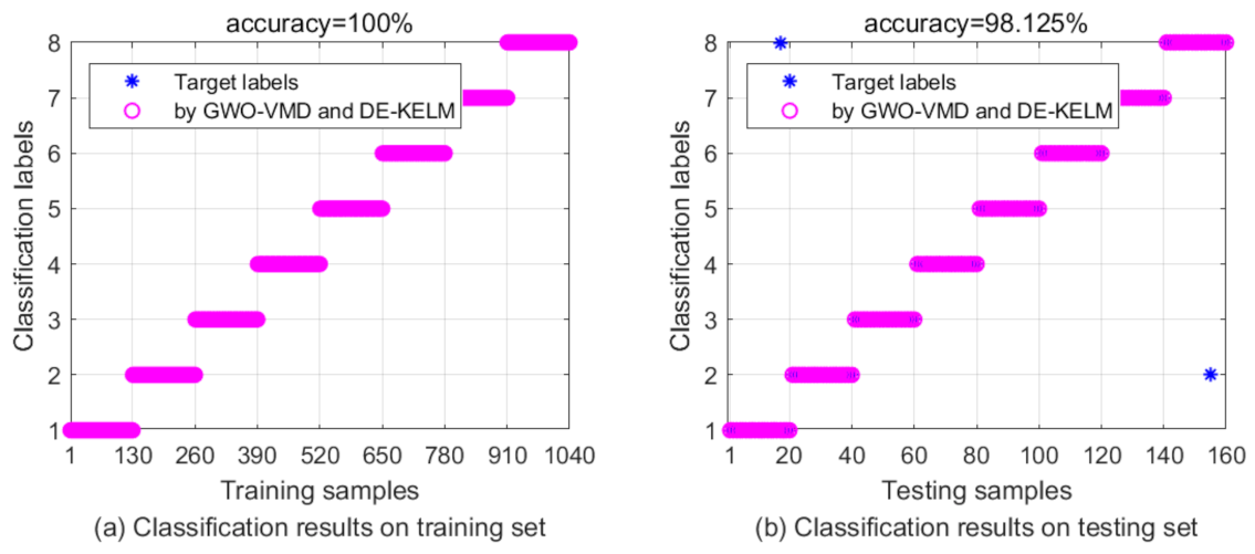
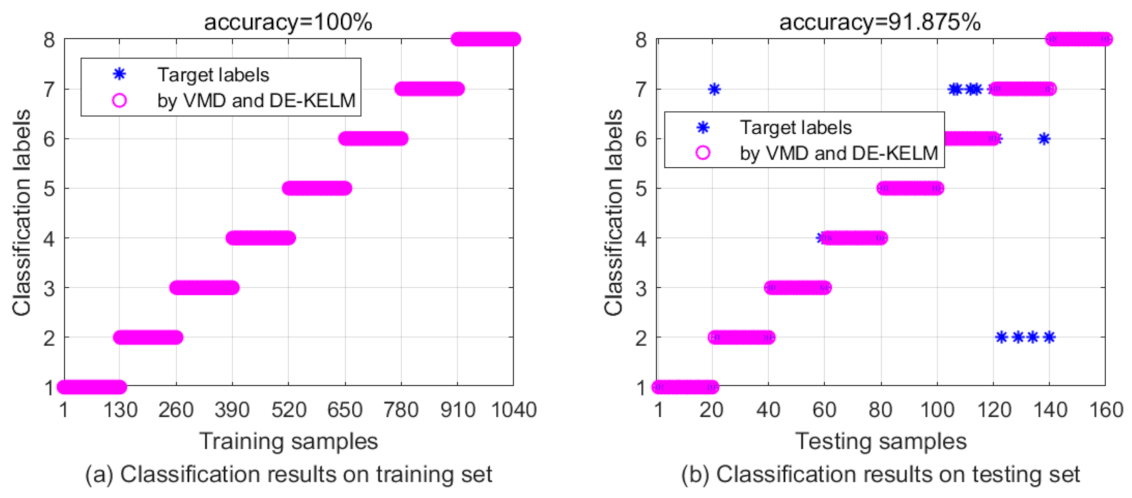
5.2.2. Fault Classification Results on the Two Sets of Feature Vectors Obtained through GWO-VMD and VMD, Respectively
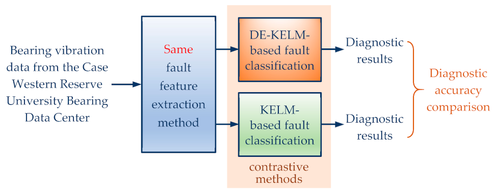
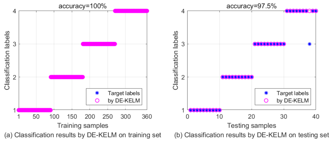
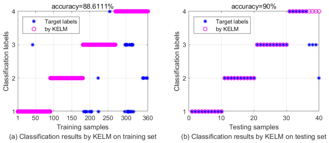
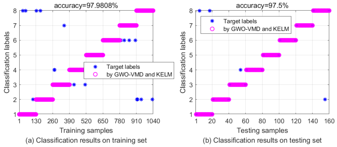
5.3. Contrast Experiment II—Fault Classification by DE-KELM and KELM, Respectively, on the Same Fault Feature Vectors
6. Conclusions and Discussion
Author Contributions
Funding
Institutional Review Board Statement
Informed Consent Statement
Data Availability Statement
Conflicts of Interest
Nomenclature
| Acronyms or Variables | Connotations |
| VMD | Variational Mode Decomposition |
| GWO | Wolf Grey Optimizer |
| KELM | Kernel Extreme Learning Machine |
| DE | Differential Evolutionary |
| IMF | Intrinsic Mode Function |
| TFA | Time-Frequency Analysis |
| STFT | Short-Time Fourier Transform |
| WVD | Wigner-Ville Distribution |
| DWT | Discrete Wavelet Transform |
| EMD | Empirical Mode Decomposition |
| PSO | Particle Swarm Optimization |
| EEMD | Ensemble Empirical Mode Decomposition |
| CNN | Convolution Neural Network |
| DRN | Deep Residual Network |
| ELM | Extreme Learning Machine |
| TL | Transfer Learning |
| SVM | Support Vector Machine |
| NN | Neural Network |
| DL | Deep Learning |
| SNR | Signal-Noise Ratio |
| PE | Permutation Entropy |
| GA | Genetic Algorithm |
| v(t) | Gearbox vibration signal |
| uk(t) | The kth IMF of v(t) |
| K | Number of imfs |
| ωk | Frequency centers of the kth IMF (Hz) |
| α | Penalty factor in VMD algorithm |
| λ | Lagrange multiplier in VMD |
| fn | Fitness function of GWO |
| kt | Kurtosis in GWO fitness function |
| Hp | Permutation entropy in GWO fitness function |
| μ | Mean value for Kurtosis calculation |
| σ | Standard deviation for Kurtosis calculation |
| m1, q | Dimensional parameters of the reconstruction matrix for Hp calculation |
| pi | Probability of each row of the reconstruction matrix |
| alpha, beta, delta, omega | Grey wolf names in their social hierarchy |
| Corr | Correlation coefficient |
| Corrth | Correlation coefficient threshold for signal reconstruction |
| v′(t) | Reconstructed gearbox vibration signal |
| vmax | Maximum amplitude of v′(t) |
| vmin | Minimum amplitude of v′(t) |
| vp | Peakedness of v′(t) |
| vpp | Peak-to-peak value of v′(t) |
| vm | Mean value of v′(t) |
| vs | Slant of v′(t) |
| vrms | Root mean square value of v′(t) |
| vr | Root square amplitude of v′(t) |
| vma | Mean of absolute value of v′(t) |
| vσ | Variance of v′(t) |
| vsf | Shape factor of v′(t) |
| vsn | Skewness of v′(t) |
| vif | Impulse factor of v′(t) |
| vcf | Crest factor of v′(t) |
| vclf | Clearance factor of v′(t) |
| vkf | Kurtosis factor of v′(t) |
| vE | Energy of v′(t) |
| vpe | Permutation entropy of v′(t) |
| Nv | Length of v′(t) |
| T | Fault feature vector |
| x(t) | Constructed experimental signal with noise |
| s(t) | Periodic impulsive signal for experiments |
| xn(t) | Gauss white noise for experiments |
| n | KELM input node number |
| L | KELM hidden layer node number |
| m | KELM output node number |
| N | Number of KELM training sample pairs |
| xi | Input vector of the ith KELM sample |
| ti | Target output of xi |
| Y | N × m output matrix of KELM |
| H | N × L output matrix of KELM hidden layer |
| ω | KELM input weight matrix |
| b | Bias vector of KELM hidden layer |
| x | KELM sample input matrix |
| β | L × m output weight matrix of KELM |
| C | Regularization factor of KELM |
| ξi | Training error of KELM |
| k(x1, x2) | Kernel function of KELM |
| f | Output function of KELM |
| g | Kernel parameter of RBF kernel |
References
- Ruan, H.; Wang, Y.; Li, X.; Qin, Y.; Tang, B.; Wang, P. A Relation-Based Semisupervised Method for Gearbox Fault Diagnosis With Limited Labeled Samples. IEEE Trans. Instrum. Meas. 2021, 70. [Google Scholar] [CrossRef]
- Jin, X.; Cheng, F.; Peng, Y.; Qiao, W.; Qu, L. Drivetrain Gearbox Fault Diagnosis VIBRATION-AND CURRENT-BASED APPROACHES. IEEE Ind. Appl. Mag. 2018, 24, 56–66. [Google Scholar] [CrossRef]
- Chen, X.; Feng, Z. Time-Frequency Analysis of Torsional Vibration Signals in Resonance Region for Planetary Gearbox Fault Diagnosis Under Variable Speed Conditions. IEEE Access 2017, 5, 21918–21926. [Google Scholar] [CrossRef]
- Zhong, D.; Guo, W.; He, D. An Intelligent Fault Diagnosis Method based on STFT and Convolutional Neural Network for Bearings Under Variable Working Conditions. In Proceedings of the 2019 Prognostics and System Health Management Conference (PHM-Qingdao), Qingdao, China, 25–27 October 2019; pp. 1–6. [Google Scholar] [CrossRef]
- Yao, J.; Zhao, J.; Deng, Y.; Langari, R. Weak Fault Feature Extraction of Rotating Machinery Based on Double-Window Spectrum Fusion Enhancement. IEEE Trans. Instrum. Meas. 2020, 69, 1029–1040. [Google Scholar] [CrossRef]
- Yang, B.; Liu, R.; Chen, X. Sparse Time-Frequency Representation for Incipient Fault Diagnosis of Wind Turbine Drive Train. IEEE Trans. Instrum. Meas. 2018, 67, 2616–2627. [Google Scholar] [CrossRef]
- Heydarzadeh, M.; Kia, S.H.; Nourani, M.; Henao, H.; Capolino, G. Gear fault diagnosis using discrete wavelet transform and deep neural networks. In Proceedings of the IECON 2016—42nd Annual Conference of the IEEE Industrial Electronics Society, Florence, Italy, 23–26 October 2016; pp. 1494–1500. [Google Scholar] [CrossRef]
- Zhao, M.; Kang, M.; Tang, B.; Pecht, M. Multiple Wavelet Coefficients Fusion in Deep Residual Networks for Fault Diagnosis. IEEE Trans. Ind. Electron. 2019, 66, 4696–4706. [Google Scholar] [CrossRef]
- Li, Y.; Xu, M.; Liang, X.; Huang, W. Application of Bandwidth EMD and Adaptive Multiscale Morphology Analysis for Incipient Fault Diagnosis of Rolling Bearings. IEEE Trans. Ind. Electron. 2017, 64, 6506–6517. [Google Scholar] [CrossRef]
- Abdelkader, R.; Kaddour, A.; Bendiabdellah, A.; Derouiche, Z. Rolling Bearing Fault Diagnosis Based on an Improved Denoising Method Using the Complete Ensemble Empirical Mode Decomposition and the Optimized Thresholding Operation. IEEE Sens. J. 2018, 18, 7166–7172. [Google Scholar] [CrossRef]
- Wang, X.-B.; Yang, Z.-X.; Yan, X.-A. Novel Particle Swarm Optimization-Based Variational Mode Decomposition Method for the Fault Diagnosis of Complex Rotating Machinery. IEEE-ASME Trans. Mechatron. 2018, 23, 68–79. [Google Scholar] [CrossRef]
- Guo, Z.; Liu, M.; Wang, Y.; Qin, H. A New Fault Diagnosis Classifier for Rolling Bearing United Multi-Scale Permutation Entropy Optimize VMD and Cuckoo Search SVM. IEEE Access 2020, 8, 153610–153629. [Google Scholar] [CrossRef]
- Wang, C.; Li, H.; Huang, G.; Ou, J. Early Fault Diagnosis for Planetary Gearbox Based on Adaptive Parameter Optimized VMD and Singular Kurtosis Difference Spectrum. IEEE Access 2019, 7, 31501–31516. [Google Scholar] [CrossRef]
- Li, F.; Li, R.; Tian, L.; Chen, L.; Liu, J. Data-driven time-frequency analysis method based on variational mode decomposition and its application to gear fault diagnosis in variable working conditions. Mech. Syst. Signal Process. 2019, 116, 462–479. [Google Scholar] [CrossRef]
- Gao, S.; Pei, Z.; Zhang, Y.; Li, T. Bearing Fault Diagnosis Based on Adaptive Convolutional Neural Network With Nesterov Momentum. IEEE Sens. J. 2021, 21, 9268–9276. [Google Scholar] [CrossRef]
- Jiang, G.; He, H.; Yan, J.; Xie, P. Multiscale Convolutional Neural Networks for Fault Diagnosis of Wind Turbine Gearbox. IEEE Trans. Ind. Electron. 2019, 66, 3196–3207. [Google Scholar] [CrossRef]
- Jin, G.; Zhu, T.; Akram, M.W.; Jin, Y.; Zhu, C. An Adaptive Anti-Noise Neural Network for Bearing Fault Diagnosis Under Noise and Varying Load Conditions. IEEE Access 2020, 8, 74793–74807. [Google Scholar] [CrossRef]
- Chen, L.; Xu, G.; Tao, T.; Wu, Q. Deep Residual Network for Identifying Bearing Fault Location and Fault Severity Concurrently. IEEE Access 2020, 8, 168026–168035. [Google Scholar] [CrossRef]
- Saufi, S.R.; Bin Ahmad, Z.A.; Leong, M.S.; Lim, M.H. Gearbox Fault Diagnosis Using a Deep Learning Model With Limited Data Sample. IEEE Trans. Ind. Inform. 2020, 16, 6263–6271. [Google Scholar] [CrossRef]
- Zhong, J.-H.; Zhang, J.; Liang, J.; Wang, H. Multi-Fault Rapid Diagnosis for Wind Turbine Gearbox Using Sparse Bayesian Extreme Learning Machine. IEEE Access 2019, 7, 773–781. [Google Scholar] [CrossRef]
- Udmale, S.S.; Singh, S.K.; Singh, R.; Sangaiah, A.K. Multi-Fault Bearing Classification Using Sensors and ConvNet-Based Transfer Learning Approach. IEEE Sens. J. 2020, 20, 1433–1444. [Google Scholar] [CrossRef]
- Zhang, X.; Han, P.; Xu, L.; Zhang, F.; Wang, Y.; Gao, L. Research on Bearing Fault Diagnosis of Wind Turbine Gearbox Based on 1DCNN-PSO-SVM. IEEE Access 2020, 8, 192248–192258. [Google Scholar] [CrossRef]
- Zhu, J.; Chen, N.; Shen, C. A New Deep Transfer Learning Method for Bearing Fault Diagnosis Under Different Working Conditions. IEEE Sens. J. 2020, 20, 8394–8402. [Google Scholar] [CrossRef]
- Yuan, L.; Lian, D.; Kang, X.; Chen, Y.; Zhai, K. Rolling Bearing Fault Diagnosis Based on Convolutional Neural Network and Support Vector Machine. IEEE Access 2020, 8, 137395–137406. [Google Scholar] [CrossRef]
- Glowacz, A.; Glowacz, W.; Kozik, J.; Piech, K.; Gutten, M.; Caesarendra, W.; Liu, H.; Brumercik, F.; Irfan, M.; Khan, Z.F. Detection of Deterioration of Three-phase Induction Motor using Vibration Signals. Meas. Sci. Rev. 2019, 19, 241–249. [Google Scholar] [CrossRef] [Green Version]
- Sun, S.; Przystupa, K.; Wei, M.; Yu, H.; Ye, Z.; Kochan, O. Fast bearing fault diagnosis of rolling element using Levy Moth-Flame optimization algorithm and Naive Bayes. Eksploat. Niezawodn. Maint. Reliab. 2020, 22, 730–740. [Google Scholar] [CrossRef]
- Yang, Z.-X.; Wang, X.-B.; Wong, P.K. Single and Simultaneous Fault Diagnosis With Application to a Multistage Gearbox: A Versatile Dual-ELM Network Approach. IEEE Trans. Ind. Inform. 2018, 14, 5245–5255. [Google Scholar] [CrossRef]
- Ren, F.; Qin, D. Investigation of the effect of manufacturing errors on dynamic characteristics of herringbone planetary gear trains. In Proceedings of the International Gear Conference 2014, Lyon, France, 26–28 August 2014; pp. 230–239. [Google Scholar] [CrossRef]
- Breeze, P. Chapter 5—Drive Trains, Gearboxes, and Generators. In Wind Power Generation, 1st ed.; Breeze, P., Ed.; Academic Press: Salt Lake City, UT, USA, 2016; pp. 41–48. ISBN 9780128040386. [Google Scholar] [CrossRef]
- Wang, C.; Li, H.; Ou, J.; Huang, G. Early Weak Fault Diagnosis of Gearbox Based on ELMD and Singular Value Decomposition. In Proceedings of the 2019 Prognostics and System Health Management Conference (PHM-Qingdao), Qingdao, China, 25–27 October 2019; pp. 1–5. [Google Scholar] [CrossRef]
- Henriquez, P.; Alonso, J.B.; Ferrer, M.A.; Travieso, C.M. Review of Automatic Fault Diagnosis Systems Using Audio and Vibration Signals. IEEE Trans. Syst. Man Cybern. Syst. 2014, 44, 642–652. [Google Scholar] [CrossRef]
- Ming, Q.; Chen, L.; Li, Y.; Yan, J. Fault Diagnosis and Status Monitoring of the Bearing. In Bearing Tribology, 1st ed.; Ming, Q., Chen, L., Li, Y., Yan, J., Eds.; Springer: Berlin/Heidelberg, Germany, 2017; pp. 239–306. ISBN 978-3-662-53095-5. [Google Scholar] [CrossRef]
- Yu, J.; Zhou, X. One-Dimensional Residual Convolutional Autoencoder Based Feature Learning for Gearbox Fault Diagnosis. IEEE Trans. Ind. Inform. 2020, 16, 6347–6358. [Google Scholar] [CrossRef]
- Dragomiretskiy, K.; Zosso, D. Variational Mode Decomposition. IEEE Trans. Signal Process. 2014, 62, 531–544. [Google Scholar] [CrossRef]
- Ma, T.; Zhang, X.; Jiang, H.; Wang, K.; Xia, L.; Guan, X. Early Fault Diagnosis of Shaft Crack Based on Double Optimization Maximum Correlated Kurtosis Deconvolution and Variational Mode Decomposition. IEEE Access 2021, 9, 14971–14982. [Google Scholar] [CrossRef]
- Liu, H.; Xiang, J. A Strategy Using Variational Mode Decomposition, L-Kurtosis and Minimum Entropy Deconvolution to Detect Mechanical Faults. IEEE Access 2019, 7, 70564–70573. [Google Scholar] [CrossRef]
- Lahmiri, S. Comparing Variational and Empirical Mode Decomposition in Forecasting Day-Ahead Energy Prices. IEEE Syst. J. 2017, 11, 1907–1910. [Google Scholar] [CrossRef]
- Mirjalili, S.; Mirjalili, S.M.; Lewis, A. Grey Wolf Optimizer. Adv. Eng. Softw. 2014, 69, 46–61. [Google Scholar] [CrossRef] [Green Version]
- Alsadie, D. TSMGWO: Optimizing Task Schedule Using Multi-Objectives Grey Wolf Optimizer for Cloud Data Centers. IEEE Access 2021, 9, 37707–37725. [Google Scholar] [CrossRef]
- Chen, X.; Yang, Y.; Cui, Z.; Shen, J. Wavelet Denoising for the Vibration Signals of Wind Turbines Based on Variational Mode Decomposition and Multiscale Permutation Entropy. IEEE Access 2020, 8, 40347–40356. [Google Scholar] [CrossRef]
- Ahmed, H.; Nandi, A.K. Compressive Sampling and Feature Ranking Framework for Bearing Fault Classification With Vibration Signals. IEEE Access 2018, 6, 44731–44746. [Google Scholar] [CrossRef]
- Li, B.; Zhang, P.; Liu, D.; Mi, S.; Ren, G. Feature extraction for roller bearing fault diagnosis based on adaptive multi-scale morphological gradient transformation. J. Vib. Shock 2011, 30, 104–108. [Google Scholar] [CrossRef]
- Shao, S.; McAleer, S.; Yan, R.; Baldi, P. Highly Accurate Machine Fault Diagnosis Using Deep Transfer Learning. IEEE Trans. Ind. Inform. 2019, 15, 2446–2455. [Google Scholar] [CrossRef]
- Huang, G.-B.; Zhou, H.; Ding, X.; Zhang, R. Extreme Learning Machine for Regression and Multiclass Classification. IEEE Trans. Syst. Man Cybern. Part B-Cybern. 2012, 42, 513–529. [Google Scholar] [CrossRef] [Green Version]
- Song, J.; Zheng, Z.; Liu, Y.; Guo, X.; Zhou, J. Wavelet Packet-based Kernel Extreme Learning Machine for Sensor Faults Diagnosis of Hypersonic Vehicle. In Proceedings of the 2018 Chinese Automation Congress (CAC), Xian, China, 30 November–2 December 2018; pp. 2017–2022. [Google Scholar] [CrossRef]
- Storn, R. On the usage of differential evolution for function optimization. In Proceedings of the North American Fuzzy Information Processing, Berkeley, CA, USA, 19–22 June 1996; pp. 519–523. [Google Scholar] [CrossRef]
- Nam, P.; Malinowski, A.; Bartczak, T. Comparative Study of Derivative Free Optimization Algorithms. IEEE Trans. Ind. Inform. 2011, 7, 592–600. [Google Scholar] [CrossRef]
- Bilal, M.; Pant, M.; Zaheer, H.; Garcia-Hernandez, L.; Abraham, A. Differential Evolution: A review of more than two decades of research. Eng. Appl. Artif. Intell. 2020, 90. [Google Scholar] [CrossRef]
- The Case Western Reserve University Bearing Data Center. Available online: https://csegroups.case.edu/bearingdatacenter/pages/welcome-case-western-reserve-university-bearing-data-center-website (accessed on 28 April 2021).
- Khamoudj, C.E.; Tayeb, F.B.-S.; Benatchba, K.; Benbouzid, M.; Djaafri, A. A Learning Variable Neighborhood Search Approach for Induction Machines Bearing Failures Detection and Diagnosis. Energies 2020, 13, 2953. [Google Scholar] [CrossRef]


| Elements | Common Faults | Causes |
|---|---|---|
| Gears | Broken Teeth |
|
| Pitting |
| |
| Cracks |
| |
| Bearings | Inner Ring Faults | Mainly include two types: wearing and pitting.
|
| Outer Ring Faults | Mainly include three types: wear, pitting and fracture.
| |
| Roller Faults |
|
| No. | Parameter Names | Notations | Mathematical Expressions |
|---|---|---|---|
| 1 | Maximum amplitude | vmax | |
| 2 | Minimum amplitude | vmin | |
| 3 | Peakedness 1 | vp | |
| 4 | Peak-to-peak value | vpp | |
| 5 | Mean value | vm | |
| 6 | Slant | vs | |
| 7 | Root mean square value | vrms | |
| 8 | Root square amplitude | vr | |
| 9 | Mean of absolute value | vma | |
| 10 | Variance | vσ | |
| 11 | Shape factor | vsf | |
| 12 | Skewness | vsn | |
| 13 | Impulse factor | vif | |
| 14 | Crest factor | vcf | |
| 15 | Clearance factor | vclf | |
| 16 | Kurtosis factor | vkf | |
| 17 | Energy | vE | |
| 18 | Permutation entropy | vpe |
| Parameters | Parameter Values or Ranges |
|---|---|
| Population number | 15 |
| Maximum iterations number | 20 |
| Range of K | [2, 8] |
| Range of α | [100, 3000] |
| IMF 1 | IMF 2 | IMF 3 | IMF 4 | IMF 5 | IMF 6 | IMF 7 | IMF 8 | |
|---|---|---|---|---|---|---|---|---|
| CORR | 0.550 | 0.744 | 0.326 | 0.266 | 0.249 | 0.243 | 0.240 | 0.229 |
| Parameters | s(t) | x(t) | Reconstructed x(t) through GWO-VMD | Reconstructed x(t) through VMD |
|---|---|---|---|---|
| Kurtosis | 7.7708 | 5.3719 | 5.4677 | 4.7667 |
| Signal–noise ratio | / | 5.0021 | 8.7756 | 8.1462 |
| RMSE | / | 0.1019 | 0.0660 | 0.0710 |
| Permutation entropy | 0.4545 | 0.9320 | 0.6145 | 0.8036 |
| Parameters | Parameters Values or Ranges |
|---|---|
| Population size | 9 |
| Maximum iteration number | 30 |
| Mutation operator | 0.7 |
| Crossover operator | 0.6 |
| Regularization coefficient C | [0.01, 100] |
| Kernel parameter g | [0.01, 10] |
| Recognized as → | Healthy | Inner Ring Fault | Outer Ring Fault | Roller Fault | Accuracy |
|---|---|---|---|---|---|
| Healthy | 10 | 0 | 0 | 0 | 100% |
| Inner ring fault | 0 | 10 | 0 | 0 | 100% |
| Outer ring fault | 0 | 0 | 10 | 0 | 100% |
| Roller fault | 0 | 0 | 1 | 9 | 90% |
| Recognized as → | Healthy | Inner Ring Fault | Outer Ring Fault | Roller Fault | Accuracy |
|---|---|---|---|---|---|
| Healthy | 10 | 0 | 0 | 0 | 100% |
| Inner ring fault | 0 | 10 | 0 | 0 | 100% |
| Outer ring fault | 0 | 0 | 10 | 0 | 100% |
| Roller fault | 0 | 1 | 3 | 6 | 60% |
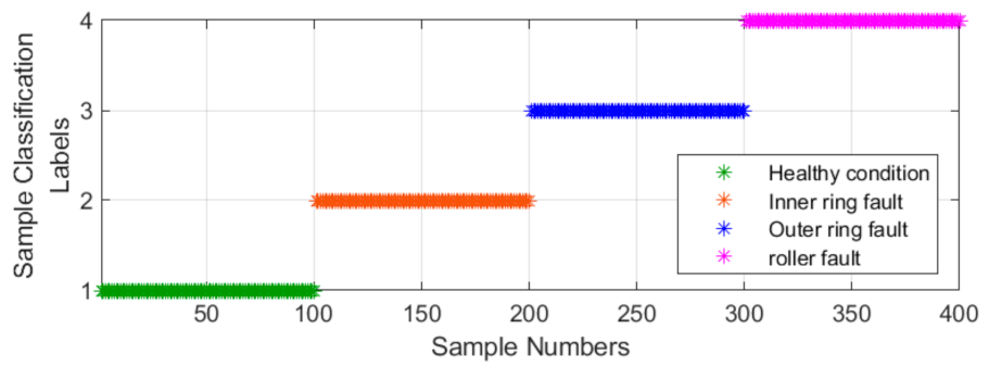
| Gearbox Elements | Classification Labels | Operating Conditions | Sample Numbers |
|---|---|---|---|
| Bearing | 1 | healthy bearing | 150 |
| 2 | inner ring fault | 150 | |
| 3 | outer ring fault | 150 | |
| 4 | roller fault | 150 | |
| Gear | 5 | healthy gear | 150 |
| 6 | pitting fault | 150 | |
| 7 | broken teeth | 150 | |
| 8 | tooth root cracks | 150 |
| Parameters | Parameter Values or Ranges |
|---|---|
| Population number | 9 |
| Maximum iterations number | 100 |
| Mode Number | [2, 15] |
| Penalty factor range | [100, 6000] |
| Gearbox Elements | Working Conditions | [K, α] |
|---|---|---|
| Bearing | healthy bearing | [11, 4018] |
| inner ring fault | [15, 139] | |
| outer ring fault | [5, 2755] | |
| roller fault | [5, 2678] | |
| Gear | healthy gear | [5, 2330] |
| pitting fault | [15, 100] | |
| broken teeth | [5, 3652] | |
| tooth root cracks | [5, 3019] |
| Gearbox Elements | Working Conditions | [K, α] |
|---|---|---|
| Bearing | healthy bearing | [3, 2000] |
| inner ring fault | [4, 2000] | |
| outer ring fault | [4, 2000] | |
| roller fault | [5, 2000] | |
| Gear | healthy gear | [4, 2000] |
| pitting fault | [5, 2000] | |
| broken teeth | [4, 2000] | |
| tooth root cracks | [4, 2000] |
| Signal Decomposition Method | Classification Accuracy of the Training Set (by DE-KELM) | Classification Accuracy of the Testing Set (by DE-KELM) |
|---|---|---|
| GWO-VMD | 100% | 98.125% |
| VMD | 100% | 91.875% |
| Fault Classification Methods | Classification Accuracy of the Training Set | Classification Accuracy of the Testing Set |
|---|---|---|
| DE-KELM | 100% | 98.125% |
| KELM | 97.9808% | 97.5% |
Publisher’s Note: MDPI stays neutral with regard to jurisdictional claims in published maps and institutional affiliations. |
© 2021 by the authors. Licensee MDPI, Basel, Switzerland. This article is an open access article distributed under the terms and conditions of the Creative Commons Attribution (CC BY) license (https://creativecommons.org/licenses/by/4.0/).
Share and Cite
Yao, G.; Wang, Y.; Benbouzid, M.; Ait-Ahmed, M. A Hybrid Gearbox Fault Diagnosis Method Based on GWO-VMD and DE-KELM. Appl. Sci. 2021, 11, 4996. https://doi.org/10.3390/app11114996
Yao G, Wang Y, Benbouzid M, Ait-Ahmed M. A Hybrid Gearbox Fault Diagnosis Method Based on GWO-VMD and DE-KELM. Applied Sciences. 2021; 11(11):4996. https://doi.org/10.3390/app11114996
Chicago/Turabian StyleYao, Gang, Yunce Wang, Mohamed Benbouzid, and Mourad Ait-Ahmed. 2021. "A Hybrid Gearbox Fault Diagnosis Method Based on GWO-VMD and DE-KELM" Applied Sciences 11, no. 11: 4996. https://doi.org/10.3390/app11114996