An Asymptotic Cyclicity Analysis of Live Autonomous Timed Event Graphs

Abstract

Designing a discrete event system converging to steady temporal patterns is an essential issue of a system with time window constraints. Until now, to analyze asymptotic stability, we have modeled a timed event graph’s dynamic behavior, transformed it into the matrix form of (max,+) algebra, and then constructed a precedence graph. This article’s aim is to provide a theoretical basis for analyzing the stability and cyclicity of timed event graphs without using (max,+) algebra. In this article, we propose converting one timed event graph to another with a dynamic behavior equivalent to that of the original without going through the conversion process. This paper also guarantees that the derived final timed event graph has the properties of a precedence graph. It then investigates the relationship between the properties of the derived precedence graph and that of the original timed event graph. Finally, we propose a method to analyze asymptotic cyclicity and stability for a given timed event graph by itself. The analysis this article provides makes it easy to analyze and improve asymptotic time patterns of tasks in a given discrete event system modeled with a live autonomous timed event graph such as repetitive production scheduling.

1. Introduction

Stability in a traditional continuous dynamic system is a property related to robustness and resilience, and designing a system to have this property is an essential issue of system control and design [1]. A stable system can eventually converge the desired steady state from an arbitrary state. To rephrase, a system can recover its original state even if it has left the steady state because of an exception or abnormality. Although stability has been introduced for continuous systems, discrete event systems, such as manufacturing systems or computer networks, also have similar stability issues such as boundedness, practical stability, and Lagrange stability in the sense of Lyapunov stability or asymptotic stability [2]. A general Petri net, a kind of a discrete event system modeling language, usually analyzes structural boundedness, a special case of Lagrange stability [3]. In that sense, the event graph, also known as a marked graph, is always a bounded Petri net, so it is stable at all times. Therefore, an event graph is rarely necessary to analyze the system’s boundedness, but it is useful for modeling a cyclic schedule for mass production, thanks to this stability [3,4,5].

However, some cyclic production systems have another type of stability issue even after modeling with event graphs. For example, a cluster tool for chemical vapor deposition (CVD) has a lower time limit, which is the minimum time required to perform a task, as well as an upper limit of wait time until the next task. The constraint forces a cluster tool to regulate fluctuations of delay or wait time between tasks to keep the product quality uniform and predictable. We call this constraint a time window constraint. Many researchers have studied how to model the cyclic schedule of a cluster tool with deterministic time using a timed event graph (TEG) to satisfy the constraint [6,7]. A TEG is a Petri net that temporizes by introducing the concept of deterministic time to places in an event graph. However, an existing system has persistent time variations or exceptions, so a TEG model analysis result cannot sometimes reflect the real one. Therefore, some studies have considered the predictable time fluctuation range when modeling and analyzing schedulability using the modified TEG [8] or have suggested a method of controlling the system within the time constraint [9].

Nevertheless, if rare exceptions occur such as time fluctuations more significant than expected or abnormality, we must quickly enable the system to converge to its normal state. Analyzing a discrete event system’s stability with such time constraints determines whether each task has asymptotically reached desired steadiness that repeats it at fixed intervals rather than analyzing the boundedness. In other words, a system that is not stable does not repeat each task at the same time interval. However, even an unstable cyclic discrete event system repeats a pattern with the time interval. We call the analysis of temporal patterns cyclicity analysis [3,10,11].

Some researchers have analyzed the cyclicity and stability with regard to the time interval pattern of TEG [3]. Specifically, if each transition repeats firing epochs asymptotically every time a specific integer d-cycles, the system is considered d-cyclic, and the one-cyclic system is considered stable. However, it is not intuitive to analyze cyclicity and stability in a TEG. Therefore, these researchers have modeled a system with a TEG and converted it into a matrix form of (max,+) algebra [8,11,12,13]. (max,+) algebra is an idempotent semiring of extended real numbers $(R\cup \{-\infty \},max,+)$ that can model and analyze the concepts of synchronization and concurrency [11,14,15,16,17]. It also has a concept of stability like the one we have explained here, so it is easy to analyze the periodicity and stability of the system [10,18,19]. However, it is not intuitive to model the dynamic behavior of the system directly with (max,+) algebra, so the analysis is performed by dualizing TEG for modeling and (max,+) algebra for analysis. Two-step analysis itself is complicated, but interpreting a (max,+) algebra model in light of the original discrete event system is also not intuitive, making improving system stability difficult.

This article uses the idea that the final result of the matrix form of (max,+) algebra for analyzing the stability is also another TEG with specific characteristics: for instance, every place has exactly one token and at most one place connecting two transitions. We first provide equivalent transformation rules between TEGs without using (max,+) algebra including place reduction rules [20] and token simplification [10]. Then, using these rules, we propose a methodology to analyze stability and cyclicity in terms of a TEG. In conclusion, we provide a direct way to calculate an asymptotic cyclicity of a given TEG and to determine whether the TEG is stable without any conversion.

This article is organized as follows: Section 2 is devoted to introducing various notations, preliminary TEG concepts, and (max,+) algebra. It also illustrates how to analyze the cyclicity and stability using a two-step analysis. Section 3 presents rules for changing to an equivalent TEG with the characteristics of a precedence graph without converting a given TEG into a matrix form. In Section 4, we suggest theoretical background finding cyclicity and stability at the TEG level. Finally, we conclude in Section 5.

2. Basic Definitions and Notations

2.1. Timed Event Graphs

This section quickly reviews the essential definitions and notations of a TEG. There are more general discussions [10,11], and an excellent survey of Petri nets [4]. A TEG is a kind of Petri net and is also known as a marked graph [21]. A TEG is defined as $\mathcal{N}=(P,T,F,H,M_0)$. It has two sets of nodes called P (a set of places) and T (a set of transitions). F is a set of arcs of a directed bipartite graph; and a Petri net where each place has exactly one input and one output transition is called an event graph. A TEG is an event graph, so when each place connects the transitions $t_i$ and $t_j$, it is often denoted as $p_{ij}$. Function $H\left(p_{ij}\right)=h_{ij}$ defined in a TEG only is a holding time function, where $h_{ij}$ is a nonnegative real number. The function’s meaning is that the token can be activated only after it enters the place $p_{ij}$ and becomes valid after $h_{ij}$ has passed. In other words, the holding time of a place defines how long a token must spend in the place before contributing to the enabling of the downstream transitions. $M_0:P\to N^{+}$ is called initial marking, where $N^{+}$ is the set of nonnegative integers.

This article uses the following symbols and notations for the set of predecessors and successors of place $p\in P$ and transition $t\in T$ [4,20]. Each place in a TEG has only one upstream transition as a predecessor and only one downstream transition as a successor:

• ${}^{•}t=\left\{p\right|(p,t)\in F\}$: the set of upstream places in transition t
• $t^{•}=\left\{p\right|(t,p)\in F\}$: the set of downstream places in transition t
• ${}^{•}p=\left\{t\right|(t,p)\in F\}$: the set of upstream transitions in place p
• $p^{•}=\left\{t\right|(p,t)\in F\}$: the set of downstream transitions in place p

A $path$ is a sequence of nodes (places and transitions) used to get from one node to another without repeating any nodes or arcs [21]. If the paths of the first and last nodes are the same, we call the nonempty path a directed cycle, simple directed cycle, or cycle for short. If all transitions in a TEG have upstream places and downstream places, we say that it is autonomous. If a cyclic schedule for mass production repeating the same task without any other external control is modeled with a TEG, the TEG can be autonomous [22]. Additionally, a live TEG can fire every transition in $M_0$ state without deadlock. The condition for which an autonomous TEG is live is that every cycle has at least one token [10].

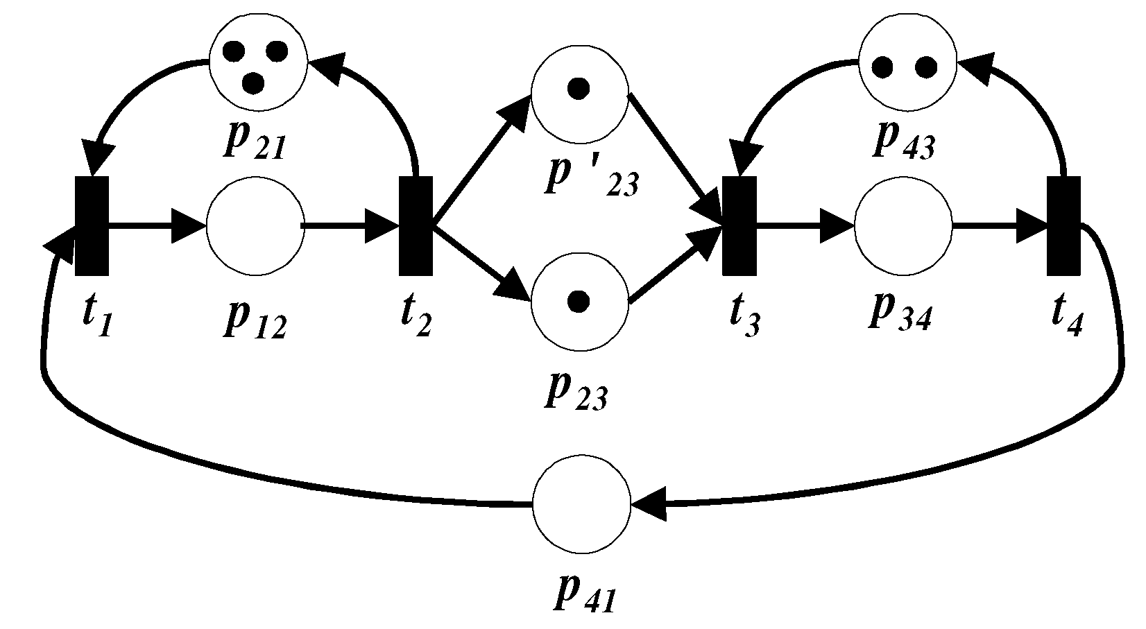
Figure 1 visualizes a TEG with seven places and four transitions. Because it is an event graph, there is exactly one pair of upstream and downstream transitions for each place, so the place connecting $t_i$ to $t_j$ is denoted as $p_{ij}$, and its holding time is represented as $h_{ij}$. However, transitions $t_2$ and $t_3$ have two places that directly connect them, for which we use denotations $p_{23}$ and $p_{23}^{\prime }$, respectively. That is, the insersection of the downstream places of $t_2$ and the upstream places of $t_3$ are $p_{23}$ and $p_{23}^{\prime }$($t_2^{•}{\cap }^{•}{t}_3=\{p_{23},p_{23}^{\prime }\}$). We extend this ${}^{•}$ notation for use in succession. ${}^{••}t$ denotes the set of upstream transitions of the upstream places of transition t (${}^{••}t={\cup }_{p\in {}^{•}t}{}^{•}p$). For example, ${}^{••}{t}_1$ is a set of $t_2$ and $t_4$ because the upstream places of $t_1$ are $p_{21}$ and $p_{41}$ and their upstream transitions are $t_2$ and $t_4$, respectively. Figure 1 has four cycles: ${\pi }_1:t_1\to p_{12}\to t_2\to p_{23}\to t_3\to p_{34}\to t_4\to p_{41}\to t_1$, ${\pi }_2:t_1\to p_{12}\to t_2\to p_{23}^{\prime }\to t_3\to p_{34}\to t_4\to p_{41}\to t_1$, ${\pi }_3:t_1\to p_{12}\to t_2\to p_{21}\to t_1$, and ${\pi }_4:t_3\to p_{34}\to t_4\to p_{43}\to t_3$. The average cycle time is defined as the sum of the holding times of the places constituting each cycle divided by the number of tokens in the cycle. For example, the cycle time of ${\pi }_1$ is $h_{12}+h_{23}+h_{34}+h_{41}$, and the cycle time of ${\pi }_3$ is $\frac{h_{12}+h_{21}}{3}$. The average cycle time of a TEG is the maximum value among the cycles’ average cycle times, and the cycle with the maximum cycle time is called a critical cycle.

2.2. (max,+) Algebra

While modeling with a TEG is intuitive, (max,+) algebra is also widely used to model the concept of synchronization and concurrency when analyzing the stability of a discrete event system. The (max,+) algebra known as the max tropical semiring is defined by $(\overline{R},\oplus ,\otimes )$ over the real number including a negative infinity and has two operators: a maximum ($\oplus :a\oplus b=max(a,b)$) and a plus ($\otimes :a\otimes b=a+b$) [14,17]. Each of these two operators is associative, commutative, and distributive. Their neutral elements of ⊕ and ⊗ correspond to a value of $-\infty$ and 0, expressed as $ϵ$ and e, respectively. TEG modeling is intuitive, whereas stability analysis is indirect, but (max,+) algebra can directly analyze the stability, whereas modeling is not intuitive. Therefore, we usually model with a TEG and then convert it to (max,+) algebra for analysis. Converting a TEG model to (max,+) algebra requires two assumptions [10]: a FIFO and an earliest starting policy. A FIFO selects the token that entered the place first when we need to determine which token has contributed to enabling the downstream transition of the place with more than one token. An earliest starting policy fires transitions immediately if all tokens stay at the minimum holding time in the upstream place. The aim of this article is to analyze whether a live autonomous TEG has asymptotical stability so that these assumptions can be established.

The first step in converting a discrete event system modeled with a TEG into a (max,+) algebra model is to express the firing schedule of transitions in a TEG in vector format. In general, the epoch when the rth firing of the transition $t_i$ occurs is denoted by $t_i^r$, so the vector $\overrightarrow{t^r}\equiv \left\{t_i^r\right|i\in T,r=1,2,...\}$ is the firing schedule of the transition in the rth cycle. In that case, the schedule satisfies the following:

$$t_j^r=ma{x}_{(i,j)\in E}\{t_i^{r-{\mu }_{ij}}+h_{ij}\}\forall j\in T,$$

(1)

while ${\mu }_{ij}$ and $h_{ij}$ indicate the number of tokens and the minimum holding time at place $p_{ij}$, respectively because we assume FIFO and the earliest epoch firing schedule. Equation (1) is an example rewritten in the form of Matrix $A\left(k\right)$ for Figure 1:

$${\overrightarrow{x}}^r=A\left(0\right){\overrightarrow{x}}^r\oplus A\left(1\right){\overrightarrow{x}}^{r-1}\oplus A\left(2\right){\overrightarrow{x}}^{r-2}\oplus A\left(3\right){\overrightarrow{x}}^{r-3},$$

(2)

where ${\overrightarrow{x}}^r\equiv {(t_1^r,t_2^r,t_3^r,t_4^r)}^{\prime }$,

$$\begin{array}{c}A\left(0\right)=\left(\begin{array}{cccc}ϵ& ϵ& ϵ& h_{41}\\ h_{12}& ϵ& ϵ& ϵ\\ ϵ& ϵ& ϵ& ϵ\\ ϵ& ϵ& h_{34}& ϵ\end{array}\right),A\left(1\right)=\left(\begin{array}{cccc}ϵ& ϵ& ϵ& ϵ\\ ϵ& ϵ& ϵ& ϵ\\ ϵ& max\{h_{23},h_{23}^{\prime }\}& ϵ& ϵ\\ ϵ& ϵ& ϵ& ϵ\end{array}\right),\hfill \\ A\left(2\right)=\left(\begin{array}{cccc}ϵ& ϵ& ϵ& ϵ\\ ϵ& ϵ& ϵ& ϵ\\ ϵ& ϵ& ϵ& h_{43}\\ ϵ& ϵ& ϵ& ϵ\end{array}\right),andA\left(3\right)=\left(\begin{array}{cccc}ϵ& h_{21}& ϵ& ϵ\\ ϵ& ϵ& ϵ& ϵ\\ ϵ& ϵ& ϵ& ϵ\\ ϵ& ϵ& ϵ& ϵ\end{array}\right).\hfill \end{array}$$

Given that Equation (2), unfortunately, uses a circular definition that defines ${\overrightarrow{x}}^r$ using ${\overrightarrow{x}}^r$, to calculate the value of ${\overrightarrow{x}}^r$, this equation must be redefined as a proper recursive definition by removing $A\left(0\right)$ and ${\overrightarrow{x}}^r$ on the right-hand side simultaneously. Therefore, the matrix needs to transform into a standard autonomous equation, which means that all matrices on the right-hand side are integrated into one matrix. The first step of this transformation is to change each matrix $A\left(k\right)$ into $\overline{A}\left(k\right)=A{\left(0\right)}^{*}\otimes A\left(k\right)$ to remove $A\left(k\right)$ and ${\overrightarrow{x}}^r$ on the right side, where $A^{*}$ is the Kleene star of A. The Kleene star is defined as $e\oplus A\oplus A^2\oplus \cdots$ where e denotes the tropical identity matrix of the same size as Matrix A [14,17].

The general standard autonomous equation form is the following:

$${\overline{\overrightarrow{x}}}^r=\overline{A}\otimes {\overline{\overrightarrow{x}}}^{r-1},$$

(3)

where ${\overline{\overrightarrow{x}}}^r=\{{\overrightarrow{x}}^r,\cdots {\overrightarrow{x}}^{r+1-M_0}\}$ and $M_0$ is the maximum initial markings of TEG $\mathcal{N}$: $\overline{A}=$$\left(\begin{array}{ccc}\overline{A}\left(1\right)& \cdots & \overline{A}\left(M_0\right)\\ e& ϵ& ϵ\\ ϵ& e& ϵ\end{array}\right).$

Generally, a standard autonomous equation’s size increases in proportion to a maximum number of initial tokens greater than its original size. Therefore, it is necessary to simplify the model’s dynamic behavior without changing it for calculation convenience. It is known that the two TEGs are said to be equivalent if there is a bijective mapping that lets two corresponding transitions of two TEGs fire simultaneously from the initial TEG set to the subset of the transformed TEG [10]. To put it another way, any observation of the dynamic behavior of the corresponding transitions of the two equivalent TEGs is identical. This article extends the concept of equivalency by not distinguishing the initial TEG from the derived TEG.

Definition 1.

Two TEGs ${\mathcal{N}}_1=(P_1,T_1,F_1,H_1,M_{01})$ and ${\mathcal{N}}_2=(P_2,T_2,F_2,H_2,M_{02})$ are said to be equivalent when the following conditions are satisfied:

• the set of the transaction of TEG $\mathcal{N}$ is a subset of the transaction of the other TEG ${\mathcal{N}}_2$ ($T_1\subseteq T_2$).
• there exists a bijective mapping that can fire the corresponding transactions of these two TEGs simultaneously.

There are many ways to reduce the size of matrix $\overline{A}$ such that the reduced TEG is equivalent to the original [10]. Using the first way, if the number of initial tokens of any place of $t^{•}$ of transition t is zero, we remove the column and the row for the transition. The other way depends on whether all elements of the column are $ϵ$. For example, the size of $\overline{A}$ is originally $12\times 12$ because Figure 1 has four transitions and, maximally, three tokens. Next, we can remove the corresponding columns and rows of $t_1$ and $t_3$ of ${\overline{A}}_1$, ${\overline{A}}_2$, and ${\overline{A}}_3$ because the transitions have no downstream place that initially has a token. Finally, we eliminate the columns whose values are all $ϵ$. In conclusion, only ${(t_2^r,t_4^r,t_2^{r-1},t_4^{r-1},t_2^{r-2})}^{\prime }$ survives, so Equation (2) is transformed into a standard autonomous equation as follows:

$${\overline{\overrightarrow{x}}}^r=\overline{A}\otimes {\overline{\overrightarrow{x}}}^{r-1}$$

(4)

$\overline{A}=$$\left(\begin{array}{ccccc}max\{h_{23},h_{23}^{\prime }\}+h_{34}+h_{41}+h_{12}& ϵ& ϵ& h_{43}+h_{34}+h_{41}+h_{12}& h_{12}+h_{21}\\ max\{h_{23},h_{23}^{\prime }\}+h_{34}& ϵ& ϵ& h_{43}+h_{34}& ϵ\\ e& ϵ& ϵ& ϵ& ϵ\\ ϵ& e& ϵ& ϵ& ϵ\\ ϵ& ϵ& e& ϵ& ϵ\\ ϵ& ϵ& ϵ& e& ϵ\end{array}\right).$

If a standard autonomous equation is visualized in TEG form again, it becomes a special form of a TEG with exactly one token in every place, so it is not necessary to represent places and tokens in the TEG. For simplicity, we use a precedence graph, which maps the columns and rows of the matrix to the graph’s nodes and maps the elements of the matrix to the weight of arcs in the graph. The precedence graph of TEG $\mathcal{N}$ is defined as $\mathcal{G}\left(\mathcal{N}\right)=(\mathcal{V},\mathcal{A},\mathcal{W})$. In $\mathcal{G}\left(\mathcal{N}\right)$, $\mathcal{V}$ is the surviving transition after conversion, $\mathcal{A}$ is the set of places in which one token connects the transitions, and $\mathcal{W}$ is the set of holding times. The precedence graph derived from the standard autonomous equation is known as an equivalent graph to the original TEG. Although the set of transitions of the precedence graph is a subset of the transitions of the original TEG, we can predict the epochs of all transitions because the corresponding transitions of the surviving ones fire at the same time, and the firing epochs of the other transitions are also decided uniquely because of the earliest starting policy. Figure 2 is a precedence graph derived from Equation (4). The node is named to represent the original TEG’s corresponding transition, and the note of an arc represents the weight.

If the precedence graph is strongly connected, we call the matrix is irreducible [17]. Additionally, if we have a real number $\lambda$ and a vector x which satisfy the equation, $A\otimes x=\lambda x$, $\lambda$ is an topical eigenvalue, and x is an tropical eigenvector associated with $\lambda$. Whereas a general matrix may have several eigenvalues, an irreducible matrix has only one eigenvalue, which we call the max(-algebraic) Perron root of A [23]. The value of $\lambda$ is the maximum cycle mean of A.

That is, the asymptotic firing epoch pattern for a given firing sequence and holding time depends on the initial firing epoch. For example, assuming that $h_{21}$ is four, $h_{43}$ is nine, and the others are one, there is more than one asymptotic firing epoch pattern of Figure 1 like Figure 3. Both schedules in Figure 3 have the same holding time and firing sequence, but the above schedule repeats every cycle; in the below schedule, the firing time pattern repeats after firing twice. In this case, the above and the below schedules are called a one-cyclic schedule and a two-cyclic schedule, respectively, and the system has an asymptotic two-cyclicity. Definition 2 gives a formal definition of cyclicity and stability.

Definition 2.

A schedule is an asymptotic d-cyclic schedule if there exists an integer d, such as ${\overrightarrow{x}}_i^{k+d}-{\overrightarrow{x}}_i^k$ is a constant, $d\lambda$, for only d that is bigger than $d^{\prime }$ and enough big integer k. In other words, the cyclicity of this schedule is d. An asymptotic 1-cyclic schedule is said to be stable or to have stability [12].

Assume that every transition fires under the earliest starting policy. If a system asymptotically converges to less than a d-cyclic schedule based on the critical cycle structure regardless of the initial firing epoch, its cyclicity is d [3]. For a given precedence graph, its cyclicity is the LCM (least common multiple) of the cyclicity of every maximal strongly connected subgraph of ${\mathcal{G}}^c$. The cyclicity of each maximal strongly connected subgraph is the GCD (greatest common divisor) of the number of arcs making up each critical cycle in the subgraph [10,17]. Additionally, if the precedence graph’s cyclicity is d, the original TEG’s firing schedule is also an asymptotic d-cyclic schedule [12]. Let us illustrate how to calculate the cyclicity with the example in Figure 2. There are four cycles in this precedence graph: ${\overline{\pi }}_1:t_{2-0}\to t_{2-0}$, ${\overline{\pi }}_2:t_{2-0}\to t_{2-1}\to t_{2-2}\to t_{2-0}$, ${\overline{\pi }}_3:t_{4-0}\to t_{4-1}\to t_{4-0}$, and ${\overline{\pi }}_4:t_{2-0}\to t_{4-0}\to t_{4-1}\to t_{2-0}$. The precedence graph can be regarded as a TEG, each of whose places has exactly one token. Each cycle’s cycle time is the sum of the weights of arcs in the cycle divided by the number of arcs. In this example, the cycle times of ${\overline{\pi }}_1,{\overline{\pi }}_2,{\overline{\pi }}_3$, and ${\overline{\pi }}_4$ are $max\{h_{23}+h_{23}^{\prime }\}+h_{34}+h_{41}+h_{12}$, $\frac{h_{21}+h_{12}}{3}$, $\frac{max\{h_{23}+h_{23}^{\prime }\}+2\times h_{34}+h_{43}+h_{41}+h_{12}}{3}$, and $\frac{h_{34}+h_{43}}{2}$. We are aware that the cycle time of ${\overline{\pi }}_4$ is the sum of ${\overline{\pi }}_1$ and ${\overline{\pi }}_3$. That is, ${\overline{\pi }}_4$ is a critical cycle, if and only if both ${\overline{\pi }}_1$ and ${\overline{\pi }}_3$ are critical. Then, we calculate the cyclicity in the order of the number of critical cycles. First, we consider the case in which there is only one critical cycle. When the critical cycle is ${\overline{\pi }}_1,{\overline{\pi }}_2,{\overline{\pi }}_3$, the cyclicity is one, three, and two, respectively. If ${\overline{\pi }}_4$ is critical, both ${\overline{\pi }}_1$ and ${\overline{\pi }}_3$ are also critical, so they are not considered now. Next, we consider when there are two critical cycles. If both ${\overline{\pi }}_1$ and ${\overline{\pi }}_3$ are critical cycles at the same time, the system is asymptotically stable because these two cycles are connected and GCD(1,3) = 1. If both ${\overline{\pi }}_2$ and ${\overline{\pi }}_3$ are critical, the cyclicity is six because the two cycles are disconnected, so LCM(3, 2) = 6. There is only one case in which three cycles are critical: ${\overline{\pi }}_1$, ${\overline{\pi }}_3$, and ${\overline{\pi }}_4$ are critical cycles at the same time. Because they are connected, the cyclicity is stable because GCD(1, 2, 3) = 1. Finally, if all four cycles are critical, all cycles are connected, and thus the schedule has stability. As a result, considering all cases where this precedence graph is stable, ${\overline{pi}}_1$ must be critical so that the system has stability. However, it is not intuitive to understand what ${\overline{pi}}_1$ means in the original TEG. We may have trouble deriving a way to improve the system from the fact that ${\overline{pi}}_1$ should be critical [12]. Therefore, this study proposes analyzing asymptotic behavior in TEGs without (max,+) algebra calculation.

3. Transformation from a TEG to Its Precedence Graph

This section explains how to transform a general TEG into a precedence graph without going through converting the (max,+) algebra to a matrix form. The precedence graph defined in Section 2 is a special type of TEG with three properties as follows [10]: There is at most one token in each place, there is always a token in all places, and there is only one place that directly connects any two transitions. Therefore, to convert from a general TEG to a precedence graph, we must separate the place with multiple initial tokens into as many places as the number of tokens, remove a place without a token by concatenation with another place, and merge parallel places that directly connect two transitions into one place.

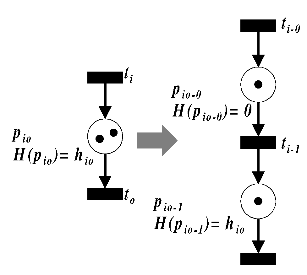
First, we explain how to remove the place with multiple tokens so each place has at most one token. There already exists a method of transforming a place with multiple tokens to another equivalent TEG [10]. Specifically, when a TEG has a place with multiple tokens, as in Figure 4, we can construct another TEG with the corresponding places with at most one token in the initial marking.

Rule 1.

Concatenation of sequence places

Precondition: 

A TEG $\mathcal{N}=(P,T,F,H,M_0)$ if there exists a place $p_{io}$ that initially has more than one token ($M_0\left(p_{io}\right)>1,\exists p_{io}\in P$).

Rule: 

A transformed equivalent TEG ${\mathcal{N}}_f=(P_f,T_f,F_f,H_f,M_{0f})$, such that

1. 

$P_f=P\cup S-\left\{p_{io}\right\}$, where $S=\left\{p_{io-j}\right|0\le j<M_0\left(p_{io}\right)\}$

2. 

$T_f=T\cup T^{\prime }-\left\{t_i\right\}$, where $T^{\prime }=\left\{t_{i-j}\right|0\le j<M_0\left(p_{io}\right)\}$

3. 

$M_0\left(p\right)=1,\forall p\in S$

4. 

${}^{•}{t}_{i-0}{=}^{•}{t}_i$

5. 

${}^{•}{t}_{i-j}=p_{io-(j-1)},\forall j,0<j<M_0\left(p_i\right)$

6. 

${}^{•}{p}_{io-j}=t_{i-j},\forall j,0\le j<M_0\left(p_i\right)$

7. 

${}^{•}{t}_o=p_{io-\{M_0\left(p_{io}\right)-1\}}$

8. 

$H\left(p_{io-j}\right)=H\left(p_{io}\right)$ if $j=M_0\left(p_{io}\right)-1$, otherwise $H\left(p_{io-j}\right)=0$

We illustrate Rule 1 with Figure 4. Steps one and two describe how sets of places and transitions are changed. Place $p_{io}$, with multiple tokens on the left of Figure 4, is replaced with as many new places as the number of initial tokens (i.e., two places with one token, $p_{io-0}$ and $p_{io-1}$). Transition $t_i$ is also divided into $t_{i-0}$ and $t_{i-1}$. Step three guarantees that each new place has exactly one token. Steps four through seven explain how to connect ${}^{•}{t}_i$ and $t_o$. The last step defines the holding time of new places. The holding time of the place $p_{io}$ in the original TEG is allocated to $p_{io-\{M_0\left(p_i\right)-1\}}$, and directly connected to the transition $t_o$. The holding time of the remaining new places is zero. If we apply this rule to all places with multiple initial tokens, the number of places and transitions increases, but it is known that the new TEG becomes equivalent to the original TEG. To sum it up, the firing epochs of the surviving transitions and the number of tokens between them do not change.

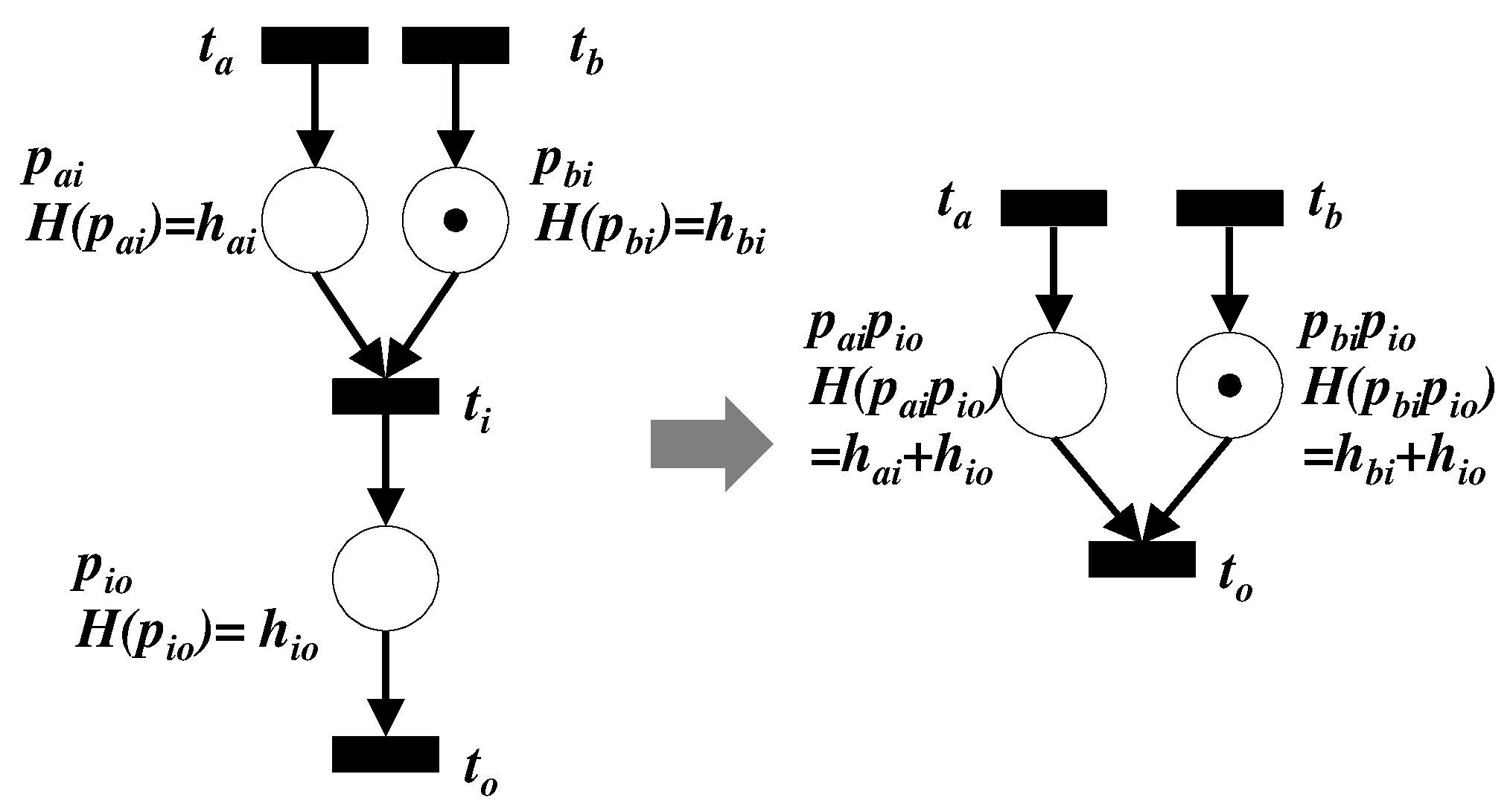
We now describe removing the place p with zero tokens from a TEG by concatenating it to another place. Because a live event graph always has the upstream transitions, the transitions belonging to ${}^{•}p$ may disappear at the same time. However, we assume that the TEG operates using the earliest starting strategy, and so the firing epoch of the removed transition is calculated automatically from the epochs of the remaining transitions. Therefore, the transformed TEG has the same dynamic behavior as the original, so they are equivalent. There are two rules for removing a zero-tokened place, depending on how many downstream places the ${}^{•}p$ has: Rules 2 and 3. First, if ${{(}^{•}{p}_{io})}^{•}=\left\{p_{io}\right\}$ as in Figure 5, the upstream transition $t_i$ in the removed place $p_{io}$ has only one downstream place, $p_{io}$ itself, Rule 2, as inspiration from the serial fusion rule [20], can be applied.

Rule 2.

The case in which both a place with a token and its upstream transition are removed.

Precondition: 

When a TEG $\mathcal{N}=(P,T,F,H,M_0)$ has Place $p_{io}$, which has no initial token, we assume that its upstream and downstream transitions are $t_i$ and $t_o$, respectively, and $t_i$ has only one downstream place $p_{io}$ ($t_i^{•}=\left\{p_{io}\right\}$)

Rule: 

A transformed equivalent TEG ${\mathcal{N}}_f=(P_f,T_f,F_f,H_f,M_{0f})$ such that

1. 

$P_f=P\cup S-\left\{p_{io}\right\}{-}^{•}{t}_i$, where $\forall p_{ji}{p}_{io},p_{ji}{p}_{io}\in S$

2. 

$T_f=T-\left\{t_i\right\}$

3. 

$M_0\left(p_{ji}{p}_{io}\right)=M_0\left(p_{ji}\right)$

4. 

${}^{•}{p}_{ji}{p}_{io}={}^{•}{p}_{ji}$

5. 

$p_{ji}{p}_{io}^{•}=p_{io}^{•}$

6. 

$H\left(p_{ji}{p}_{io}\right)=H\left(p_{ji}\right)+H\left(p_{io}\right)$

Figure 5 shows an example in which place $p_{io}$ without any token is concatenated to ${}^{••}{p}_{io}$, and its upstream transition $t_i$ is removed. As a result, the number of places and transitions of the new equivalent TEG decreases by one. The new place is named $p_{ai}{p}_{io}$ and $p_{bi}{p}_{io}$ in succession, with two concatenated places’ names, and their initial markings are the same as $p_{ai}$ and $p_{bi}$, respectively. Their holding times are the sum of two holding times of the merged places (i.e., $h_{ai}+h_{io}$ and $h_{bi}+h_{io}$). Lemma 1 proves that the TEG derived by Rule 2 is equivalent to the original TEG.

Lemma 1.

TEG $\mathcal{N}$ derived by Rule 2 is equivalent to ${\mathcal{N}}_f$.

Proof. 

The set of transitions of TEG ${\mathcal{N}}_f$ newly derived by Rule 2 is $T_f=T-\left\{t_i\right\}$, which is a subset of the original transition set. We denote the rth firing epoch of the transition $t_i$ as $t_i^r$ and then assume that place $p_{io}$ has no initial token. That is, $t_o^r=t_i^r+H\left(p_{io}\right)$ at the rth firing epoch of $t_o$. The rth firing epoch of $t_o$ of the newly created TEG ${\mathcal{N}}_f$ is changed to

$$t_o^r=\underset{p_{ji}{\in }^{•}{t}_i}{max}\{H\left(p_{ji}\right)+H\left(p_{io}\right)+t_j^{r-M_0\left(p_{ji}\right)}\}.$$

(5)

If firing epochs of transitions other than $t_o$ are the same, the two TEGs are equivalent by Definition 1, given that the number of tokens between the remaining transitions and firing epochs of $t_o$ do not change. □

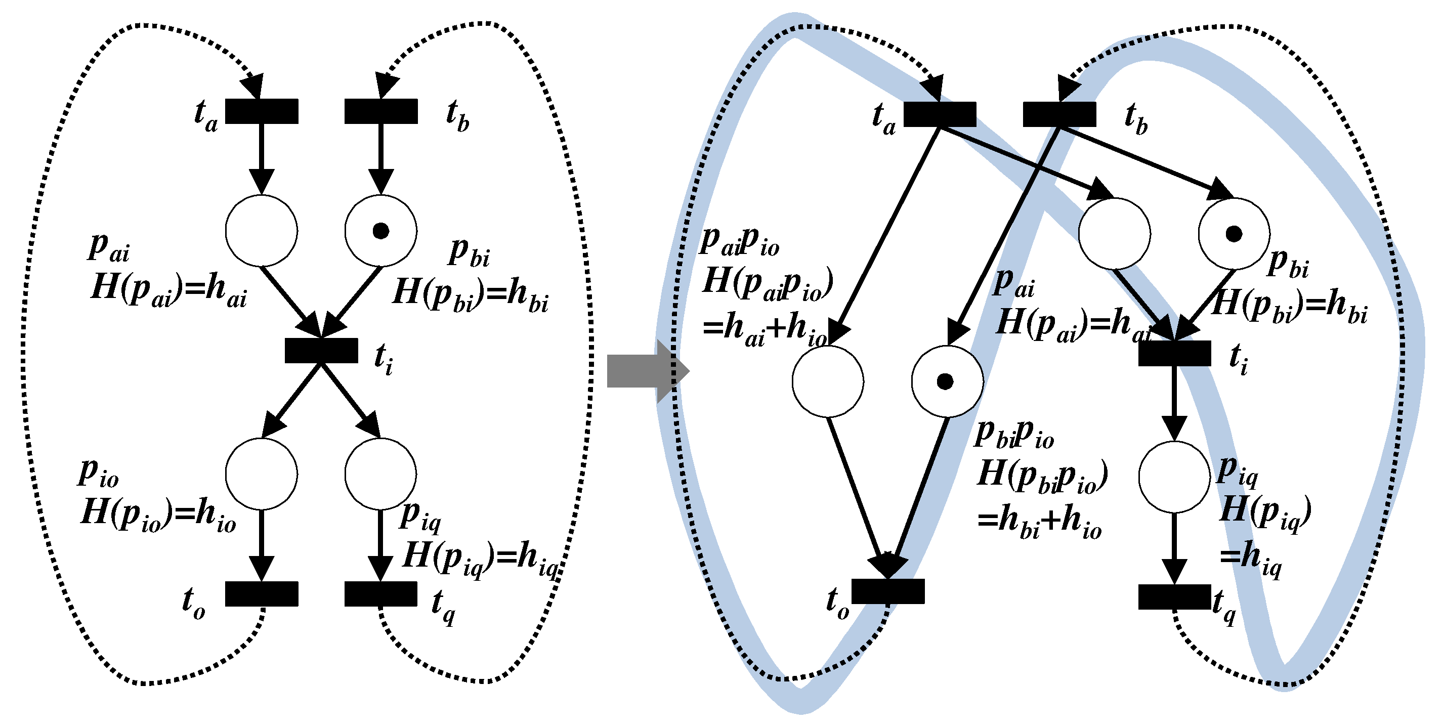
The next rule removes zero-tokened $p_{io}$, whose upstream transition $t_i$ has multiple downstream places. After applying this rule, a place without a token in the original TEG is concatenated to the preceding places ${}^{••}{p}_{io}$, but the upstream transition $t_i$ does not disappear.

Rule 3.

The case in which a place with a token is removed, but its upstream transition survives.

Precondition: 

When a TEG $\mathcal{N}=(P,T,F,H,M_0)$ has Place $p_{io}$, which has no initial token, we assume that its upstream and downstream transitions are $t_i$ and $t_o$, respectively, and $t_i$ has multiple downstream places, unlike Rule 2 ($t_i^{•}-\left\{p_{io}\right\}\ne \varnothing$).

Rule: 

A transformed equivalent TEG ${\mathcal{N}}_f=(P_f,T,F_f,H_f,M_{0f})$ such that

1. 

$P_f=P\cup S-\left\{p_{io}\right\}$, where $\forall p_{ji}{p}_{io},p_{ji}{p}_{io}\in S$

2. 

$t_i^{•}=t_i^{•}-\left\{p_{io}\right\}$

3. 

$M_0\left(p_{ji}{p}_{io}\right)=M_0\left(p_{ji}\right)$

4. 

${}^{•}{p}_{ji}{p}_{io}={}^{•}{p}_{ji}$

5. 

$p_{ji}{p}_{io}^{•}=p_{io}^{•}$

6. 

$H\left(p_{ji}{p}_{io}\right)=H\left(p_{ji}\right)+H\left(p_{io}\right)$.

Rule 3 is similar to Rule 2 in that a place without a token is concatenated to the upstream places of its upstream transition, but its upstream transition has other downstream places, so it is making the two rules different in that the transition survives after applying the rule. Figure 6 shows an example in which place $p_{io}$ is replaced with $p_{ai}{p}_{io}$ and $p_{bi}{p}_{io}$ according to Rule 3. This example does not remove the upstream transition $t_i$ of $p_{io}$, as opposed to Rule 2. The number of transitions of both TEGs before and after applying the rule is the same as five, but the total number of places increases by the number of upstream places of $t_i$. The holding times, the initial markings, and the naming convention of transformed places are the same as those in Rule 2. Lemma 2 proves that the TEG after applying Rule 3 is equivalent to the original TEG.

Lemma 2.

TEG $\mathcal{N}$ derived by Rule 3 is equivalent to ${\mathcal{N}}_f$.

Proof. 

The set of transitions of TEG ${\mathcal{N}}_f$ transformed by Rule 3 is the same as the original transition set except for the connection relationship with the place. The rule does not change any of the downstream places of the upstream transition of place $p_{io}$ by Rule 3 except $t_i$ and $p_{io}$, so $\left\{t_i^{••}\right\}-\left\{t_o\right\}$ has the same firing epoch after applying the rule. $t_o$ fires at the same time as before the rule was applied for the same reason as in Lemma 1. In addition, the initial marking of the new place $M_0\left(p_{ji}{p}_{io}\right)=M_0\left(p_{ji}\right)$, where $p_{ji}{\in }^{•}{t}_i$, so the number of tokens between $t_j$ and $t_o$ has not changed. That is, the transformed TEG from applying Rule 3 is equivalent to the original TEG. □

Finally, we examine the case in which merging multiple places with the same number of tokens connecting two consecutive transitions into one, as shown in Figure 7. We can apply Rule 4 for this case.

Rule 4. 

Merging of parallel places.

Precondition: 

There is an arbitrary subset S of places in which the initial token number, the upstream transition $t_i$ and the downstream transition $t_o$ of all places belonging to S are the same.

Rule: 

All places belonging to the set of places S may be replaced by a single place, specifically a transformed equivalent TEG ${\mathcal{N}}_f=(P_f,T,F_f,H_f,M_{0f})$ such that

1

$P_f=P\cup \{p_{io}^0|\cdots |p_{io}^k\}-S$

2

$M_0\left(p_{io}\right)=M_0(p_{io}^0|\cdots |p_{io}^k)$

3

${}^{•}(p_{io}^0|\cdots |p_{io}^k)=t_i$

4

$(p_{io}^0|\cdots |p_{io}^k{)}^{•}=t_o$

5

$H(p_{io}^0|\cdots |p_{io}^k)=\underset{\forall p_{io}\in S}{max}H\left(p_{io}\right)$.

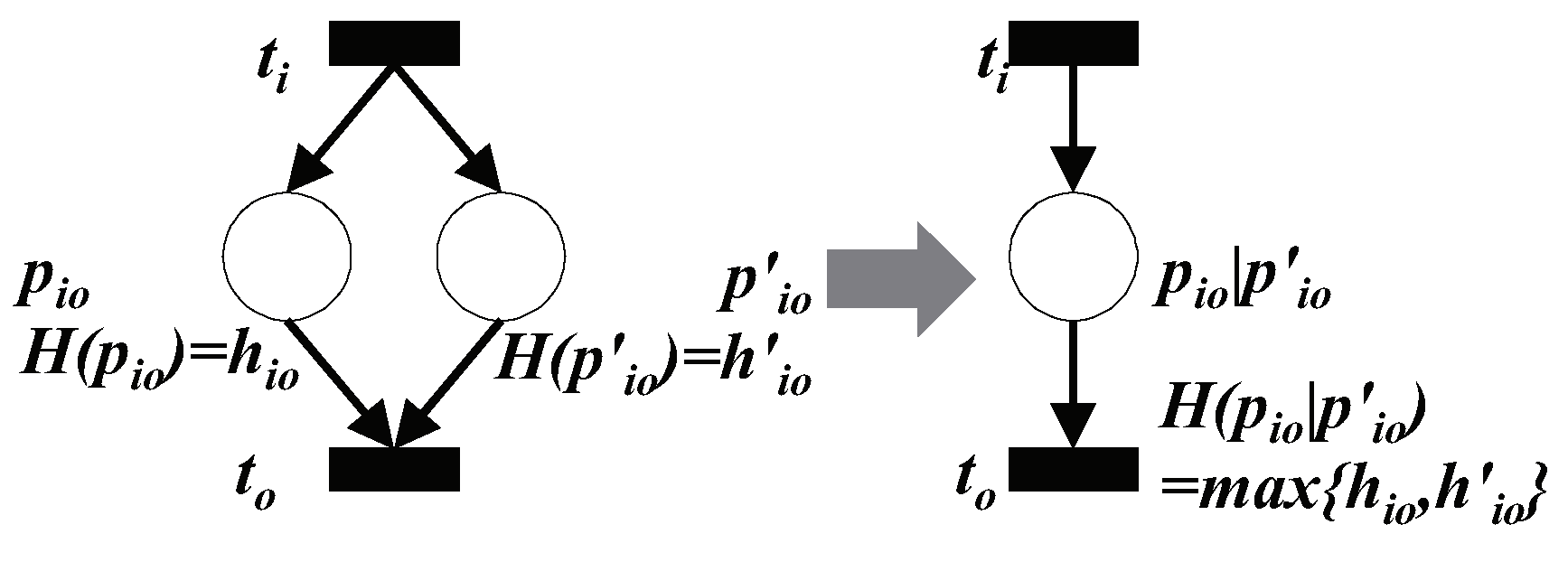
By way of explanation, if we apply Rule 4, the new place’s holding time is the maximum of the original places, and its upstream transition and downstream transition do not change. We denote | notation to indicate which places are merged in the place newly created by Rule 4 when parallel places directly connect two transitions. Figure 7 illustrates how zero-tokened places $p_{io}$ and $p_{io}^{\prime }$, which directly connect $t_i$ and $t_o$ merge to form $p_{io}|p_{io}^{\prime }$. Its holding time becomes the maximum value of the holding time of $p_{io}$ and $p_{io}^{\prime }$. Lemma 3 proves that the new TEG after this transformation is equivalent to the one in existence before the application of Rule 4.

Lemma 3.

TEG $\mathcal{N}$ transformed by Rule 4 is equivalent to ${\mathcal{N}}_f$.

Proof. 

When all places connect from $t_i$ to $t_o$ and have the same number of tokens, we call them parallel places, and their set is denoted as S ($S{=}^{•}{t}_o\cap t_i^{•}$). All places included in the set of the upstream places of $t_o$ but not belonging to S is denoted as $S^{\prime }$ ($S^{\prime }={}^{•}{t}_o-S=\left\{p_{jo}\right|p_{jo}\in S^{\prime }\}$). Under this assumption, the rth firing epoch of $t_o$ after applying Rule 4 is changed from Equation (6) to Equation (7):

$$t_o^r=max\{\underset{p_{io}\in S}{max}\{H\left(p_{io}\right)+t_i^{r-M}\},\underset{p_{jo}\in S^{\prime }}{max}\{H\left(p_{jo}\right)+{{(}^{•}{p}_{jo})}^{r-M_o\left(p_{jo}\right)}\}\}.$$

(6)

$$t_o^r=max\{\underset{p_{io}\in S}{max}\left\{H\left(p_{io}\right)\right\}+t_i^{r-M},\underset{p_{jo}\in S^{\prime }}{max}\{H\left(p_{jo}\right)+{{(}^{•}{p}_{jo})}^{r-M_o\left(p_{jo}\right)}\}\}.$$

(7)

If the firing epochs of the other transitions except for $t_o$ are the same as before, the firing epoch of $t_o$ is also the same. Therefore, by Definition 1, the TEGs are equivalent. □

This paper proposes four rules to simplify the equivalent TEG. If we repeatedly apply the transformation rules proposed in this paper, we can finally derive a TEG equivalent to the original TEG to satisfy the properties of the precedence graph. We have already proved that a transformed TEG is always equivalent even after applying any of Rules 1–4. Therefore, we now show that repeatedly applying rules can make a TEG eventually satisfy the precedence graph’s properties. In other words, every place has exactly one token in the final TEG, and the number of places directly connecting any two transitions is at most one. To prove that every place has exactly one token, we first show that any place has at most one token by contradiction. In other words, we hypothesize that there remains a place with two or more tokens no matter how often the rule is applied. In this case, we can decrease the number of tokens to one by applying Rule 1 to a place with multiple tokens. This decrease violates the hypothesis that, no matter how much the rule is applied, a place with multiple tokens cannot be removed. Therefore, we can always make the number of tokens fewer than one in all places. Next, we prove that there is at least one token in every place. The event graph, which this paper considers, is autonomous, so every place has its input transition. Therefore, we prove that every place has at least one token by showing that every transition has only its downstream places with tokens. When there is a transition with a downstream place without tokens, we divide the cases by the number of its downstream places. If the transition has only one downstream place without tokens, we can remove the transition using Rule 2. After that, a TEG has no transition, whose downstream place has no token. If the transition has multiple downstream places, we can remove a downstream place without tokens by applying Rule 3. If the transition has multiple downstream places with no tokens, we can remove them by applying Rule 3 repeatedly until every downstream place has at least one token. This way, we can make sure every place has at least one token. Finally, we prove by contradiction that there is at most one place that directly connects two arbitrary transitions. Expressly, we assume that no matter how many times rules are applied, there still remain multiple places that directly connect two transitions. We can make the number of tokens in those places at most one by Rule 1. If a place with more than two tokens exists, it does not link directly between the transitions because the place is replaced with a series of other places and transitions. Next, places that connect directly connected transitions are merged according to the number of tokens by Rule 4. After applying Rule 4, if the places are merged into one, the assumption that we cannot merge places between two transitions into one is violated. If there are two places, one place has a token and the other has no token. Rule 3 can make it so there is only one place between the transitions by removing the place without tokens, so this situation also violates the assumption. Therefore, we can make a TEG in which every pair of transitions is connected by one place at most. In conclusion, if we apply Rules 1–4 repeatedly to a live autonomous TEG, we can achieve a TEG equivalent to the original and eventually have the properties of a precedent graph.

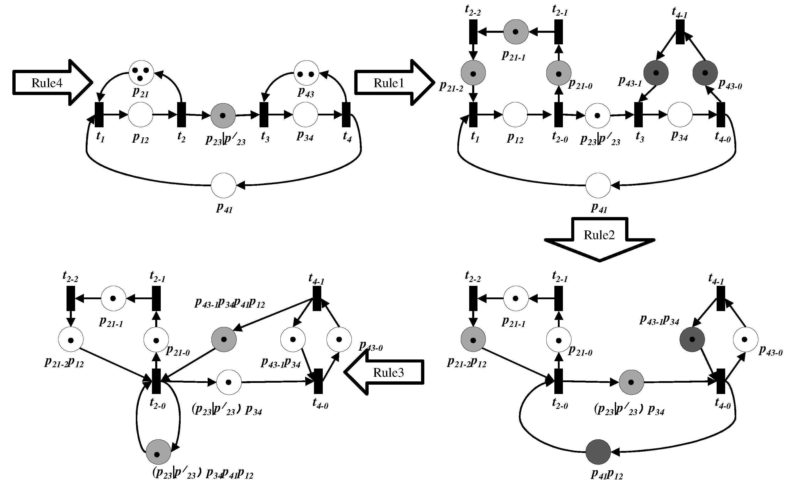
Figure 8 illustrates the process of deriving a precedence graph from Figure 1 while repeatedly applying transformation rules. For better understanding, the newly created place in each step is highlighted in gray. First, parallel places $p_{23}$ and $p_{23}^{\prime }$ are merged using Rule 4. In the next step, places with multiple tokens $p_{21}$ and $p_{43}$ are divided into corresponding places by Rule 1: ($p_{21}\Rightarrow p_{21-0}$, $p_{21-1}$ and $p_{21-2}$) and ($p_{43}\Rightarrow p_{43-0}$ and $p_{43-1}$). Now, there are currently three places without tokens, $p_{12}$, $p_{34}$, and $p_{41}$, so we must remove them using Rules 2 and 3. The upstream transition of each of places $p_{12}$ and $p_{32}$ has only one downstream place, so Rule 2 is applied. For $p_{12}$, the upstream transition $t_1$ is removed, and the place $p_{12}$ is concatenated to $p_{21-2}$ and $p_{41}$, which belong to the upstream places of $t_1$. Like $p_{12}$, $p_{34}$ is concatenated with $p_{43-1}$ and $p_{23}|p_{23}^{\prime }$ by removing Transition $t_3$. Now, there only remains one place without tokens, $p_{41}{p}_{12}$. Its upstream transition is $t_{4-0}$, which has two downstream places, $p_{41}{p}_{12}$ and $p_{43-0}$. After Rule 3 is applied, two new places are created by concatenating $p_{41}{p}_{12}$ with the upstream places of $t_{4-0}$, $\left(p_{23}\right|p_{23}^{\prime })p_{34}$ and $p_{43-1}{p}_{34}$, respectively. The TEG in the last step of Figure 8 has the precedence graph’s properties and is isomorphic with the precedence graph in Figure 2.

4. Stability Analysis of a TEG

This section analyzes how the original TEG $\mathcal{N}=(P,T,F,H,M_0)$ properties affect the derived precedence graph $\mathcal{G}\left(\mathcal{N}\right)=(\mathcal{V},\mathcal{A},\mathcal{W})$ and suggests how to calculate the cyclicity of a live autonomous TEG. First, we investigate which transitions of $\mathcal{G}\left(\mathcal{N}\right)$ become corresponding vertices or decompose into multiple corresponding vertices. Lemma 4 determines which transition survives as the vertex of $\mathcal{G}\left(\mathcal{N}\right)$.

Lemma 4.

If and only if a transition of TEG $\mathcal{N}$ has at least one downstream place with a token, the transition has corresponding vertices in $\mathcal{G}\left(\mathcal{N}\right)$.

Proof. 

To prove this lemma, we show that, if any downstream place has a token, we cannot remove its upstream transition, and if there is no place with a token among the downstream places, the transition is always removed.

First, we prove that a transition whose downstream places have tokens is not removed. Only Rule 2 eliminates a transition after applying the rule. The precondition of the rule is that there is no token in the downstream place of the transition. Even when the downstream transition of its downstream place has been previously eliminated, the token cannot exist in the new downstream place because it occurs only as a result of Rule 2, so the place does not have a token. Therefore, a corresponding transition exists in the precedence graph derived by repeatedly applying transformation rules when one or more downstream places have tokens.

Next, we show that the transition without a token in the downstream place is finally not included in the precedence graph. If all downstream places of a transition have no tokens, Rule 3 is applied repeatedly until only one downstream place is left, and then the transition can be eliminated using Rule 2. Therefore, a transition whose downstream places have no tokens is eventually removed. □

For example, let’s check how to map the transitions of TEG $\mathcal{N}$ in Figure 1 to the vertices of precedence graph $\mathcal{G}\left(\mathcal{N}\right)$ in Figure 2. The only transitions with tokened downstream places are $t_2$ and $t_4$ in the TEG $\mathcal{N}$, and their corresponding vertices are as follows: $t_2\Rightarrow$($t_{2-1}$, $t_{2-2}$ and $t_{2-3}$), and $t_4\Rightarrow$($t_{4-0}$ and $t_{4-1}$). In other words, only the corresponding vertices of $t_2$ and $t_4$ of the precedence graph have downstream place tokens.

Next, we examine the view of the cycle. Because a live autonomous TEG has a token for each cycle, at least one transition survives as a corresponding vertex for each cycle. In this example, the cycles ${\pi }_1$ and ${\pi }_2$ of $\mathcal{N}$ go through both $t_2$ and $t_4$, and the cycles ${\pi }_3$ and ${\pi }_4$ go through both $t_2$ and $t_4$. Looking at the corresponding transition of the vertex included in each cycle of $\mathcal{G}\left(\mathcal{N}\right)$, cycles ${\overline{\pi }}_1$ and ${\overline{\pi }}_2$ have only $t_2$, and ${\overline{\pi }}_3$ is related to $t_4$. Cycle ${\overline{\pi }}_4$ is related to both $t_2$ and $t_4$. Then, what is the relationship between the cycles of $\mathcal{N}$ and $\mathcal{G}\left(\mathcal{N}\right)$? Lemma 5 investigates the relationship between the two.

Lemma 5.

If a cycle exists in the original TEG $\mathcal{N}$, a corresponding cycle exists in the derived precedence graph $\mathcal{G}\left(\mathcal{N}\right)$. If there is a cycle in the derived $\mathcal{G}\left(\mathcal{N}\right)$, there is a corresponding cycle and concatenation of corresponding cycles in $\mathcal{N}$.

Proof. 

We prove this lemma by observing how each rule changes a cycle based on how reachable the transition is. That one transition is reachable from another means that a path exists between them.

First, we prove that Rule 1 does not change the reachability among transitions. According to the rule, the corresponding transitions of $t_i$ denoted as $t_{i-j}$ are reachable from $t_{i-0}$ by 5–8 of Rule 1. Additionally, only transitions having a path to $t_i$ have a path to $t_{i-j}$ and vice versa because the sets of upstream places of $t_i$ and $t_{i-o}$ are the same. For the same reason, a transition is reachable from $t_{i-j}$ after applying the rule if and only if it is reachable from $t_o$ before doing so. From the point of view of a cycle, if $t_i$ belongs to a particular cycle before applying the rule, its corresponding transitions $t_{i-j}$ belong to the corresponding cycle. In other words, Rule 1 does not change the transition’s reachability, so we can find the corresponding cycle of any cycle after applying the rule. This rule does not change the number of tokens or the cycle times either. Although the number of places increases by the number of tokens, the number of tokens in the newly created place is one for each, so the numbers of tokens of both TEG are identical. The sum of the holding time of the corresponding cycle is not changed because this rule decomposes one place into multiple places, but only one place $p_{io-\{M_0\left(p_{io}\right)-1\}}$ has the same holding time as the original place $p_{io}$, and the rest of the places $p_{io-j}$ have zero holding times for a positive integer j that is smaller than $M_0\left(p_i\right)$. As a result, the number of cycles does not change after applying Rule 1, and the cycle time of the corresponding cycles is the same as the original cycle times.

Rule 2 also does not change reachability, except for the direct connections of ${}^{••}{t}_i$ and $t_o$ caused by the removal of $t_i$. Therefore, the sets of transitions reachable to ${}^{••}{t}_i$ and reachable by $t_o$ do not change, so the reachabilities between surviving transitions remain. From the viewpoint of the cycle, the cycles including $t_i$ for the transitions in ${}^{••}{t}_i$ directly connect to $t_o$ after applying Rule 2. The cycle has the same cycle time and sum of tokens as the original because $p_{ji}{p}_{io}$ calculates the value by summing tokens of concatenated places $p_{ji}$ and $p_{io}$ where $t_j$ belongs to ${}^{••}{t}_i$. In summary, Rule 2 does not change the number of cycles or the cycle time of each cycle.

After applying Rule 3, the directly connected path from $t_i$ to $t_o$ disappears when the place $p_{io}$ is removed. The result excludes $t_i$ in the cycles that include both $t_i$ and $t_o$ initially. This removal divides the cycles formerly including $t_i$ into two kinds of cycles: cycles including the new place that directly connects ${}^{••}{t}_i$ to $t_o$ and the unchanged cycles that still include $t_i$. Additionally, this rule creates new cycles that concatenate these two types of cycles not to pass the same arc or transition except for $t_i$. In other words, we build a new cycle by connecting two different kinds of cycles after switching the upstream place of $t_i$ in two cycles. Therefore, the total holding time and number of tokens of the created cycle are the sums of the data for two connected cycles. To help understand the proof, we illustrate how Rule 6 increases cycles using Figure 6. In the figure, the dotted line and the gray line denote the arbitrary path to create a cycle and the newly created cycle, respectively. Assume that $t_a$ and $t_b$ belong to ${}^{••}{t}_i$ and $t_o$ and $t_q$ are in $t_i^{••}$, where $t_a$ is not $t_b$ and $t_o$ is also not $t_q$. The left TEG has two cycles with $p_{io}$ and $p_{iq}$, which share no transition except $t_i$. The right TEG has an additional new cycle connecting them in the following way: decrease the cycle in the sequence of $t_b$, the new place $p_{bi}{p}_{io}$, $t_o$, the path removing $p_{io}$ from the cycle including $p_{ai}$ and $p_{io}$ ($t_o\to \cdots \to t_a\to p_{ai}\to t_i$), and the path removing $p_{bi}$ from the cycle including $p_{bi}$ and $p_{iq}$ ($p_{iq}\to \cdots \to t_b$).

Rule 4 does not change transitions. It merges places whose upstream transition, downstream transition, and token number are identical. Given that these merged places have the same upstream transition and downstream transition, the reachability does not change. That is, if and only if there was a cycle that a merged place $p_{io}$ could make with $t_o\to \cdots \to t_i$, all other merged places also make a cycle use the same path. We can also compose a cycle using the new place with the same path. Thus, if the original TEG has $n\times m$ cycles because there are m different paths from $t_o$ to $t_i$ and n places are merged by Rule 4, the number of cycles decreases to m after the rule is applied. The cycle time of transformed TEG becomes the maximum cycle time of n merged cycles. The number of tokens in the corresponding cycle does not change. □

We can now comprehend the meaning of the proof of Lemma 5 using Figure 8. The first step merges places $p_{23}$ and $p_{23}^{\prime }$ by applying Rule 4, so the cycles ${\pi }_1$ and ${\pi }_2$ are combined into one cycle. The cycle time of the combined cycle is the same as the maximum of cycles ${\pi }_1$ and ${\pi }_2$, and its token numbers are unchanged. Other cycles ${\pi }_3$ and ${\pi }_4$ remain, so the number of cycles decreases to three. The next step decomposes the corresponding transitions from $t_2$ and $t_4$ by Rule 1. Consequently, cycles ${\pi }_3$ and ${\pi }_4$ increase the number of transitions and places, but the transformed TEG keeps the cycles and cycle times. The third step removes the places $p_{12}$ and $p_{34}$ using Rule 2. Cycle ${\pi }_3$ becomes ${\overline{\pi }}_2$, each of whose places has exactly one token. Cycle ${\overline{\pi }}_2$ still keeps the number of tokens and the sum of the holding times of places that make up the cycle, so the cycle times of ${\pi }_3$ and ${\overline{\pi }}_2$ are the same. Similarly, ${\pi }_4$ becomes ${\overline{\pi }}_3$, and their cycle times are equal. In the final step, applying Rule 3 causes the place $p_{41}{p}_{12}$ to disappear. As a result, we can remove all zero-tokened places in the combined cycle from the first step, and we call it ${\overline{\pi }}_1$.

The cycle time of ${\overline{\pi }}_1$ is still the maximum of ${\pi }_1$ and ${\pi }_2$, and the number of tokens is maintained as one. Additionally, this step creates a new cycle ${\overline{\pi }}_4$ by connecting ${\overline{\pi }}_1$ and ${\overline{\pi }}_3$. The newly created ${\overline{\pi }}_4$ has the cycle time of the sum of the maximum cycle time of cycles ${\pi }_1$ and ${\pi }_2$ plus ${\pi }_4$. Its number of tokens is three, which is the sum of the number of tokens in the connected cycle ${\overline{\pi }}_1$ and ${\overline{\pi }}_3$. As such, Figure 8 satisfies Lemma 5. From the proof of Lemma 5, we can also derive Collarories 1–3.

Corollary 1.

If a cycle $\overline{\pi }$ of a precedence graph $\mathcal{G}\left(\mathcal{N}\right)$ corresponds to one cycle π of the original TEG $\mathcal{N}$, its length is the same as the number of tokens of π. By comparison, if a cycle $\overline{\pi }$ is the concatenation of more than two cycles ${\pi }_i,\cdots {\pi }_j$, its length equals the sum of the number of tokens in ${\pi }_i\cdots {\pi }_j$.

Corollary 2.

If a cycle $\overline{\pi }$ of a precedence graph $\mathcal{G}\left(\mathcal{N}\right)$ corresponds to one cycle π of the original TEG $\mathcal{N}$, the sum of the holding times of the places it comprises is the same as the sum of the holding times of the places that make up π. If $\overline{\pi }$ is derived from the concatenation of multiple cycles ${\pi }_i,\cdots {\pi }_j$, the sum of the holding times of all places constituting $\overline{\pi }$ equals the holding times of the places included in ${\pi }_i,\cdots {\pi }_j$. However, if there are places merged by Rule 4 among ${\pi }_i,\cdots {\pi }_j$, only the maximum value is added without adding their individual values.

Corollary 3.

Rules 1–4 do not change the reachability between transitions.

Proof. 

Lemma 5 shows that the reachability is unchanged except in the case of Rule 3. Rule 3 eliminates the place directly connecting $t_o$ from $t_i$, so we suspect that $t_o$ may no longer reach $t_i$. However, given that every transition in a live autonomous TEG is included in any cycle, $t_i$ has a path to ${}^{••}{t}_i$, and ${}^{••}{t}_i$ can connect to $t_o$ via new places. Therefore, there is a path, $t_i\to \cdots \to {}^{••}{t}_i\to$ new place $\to t_o$. In conclusion, Rule 3 also does not change the reachability. □

It is known that the stationary behavior is d-cyclic if the transitions of a strongly connected TEG fire under the earliest starting strategy [3]. From the lemmas and corollaries proved thus far, we can find the cyclicity in a live autonomous TEG as Theorem 1.

Theorem 1.

When a live autonomous TEG $\mathcal{N}$ is strongly connected, the cyclicity of a TEG $\mathcal{N}$ is the LCM of the cyclicities of all maximal strongly connected subgraphs of ${\mathcal{N}}^c$, which is a critical graph consisting only of critical cycles. The cyclicity of each maximal strongly connected subgraph of ${\mathcal{N}}^c$ is the GCD of the number of tokens of all its cycles. In other words, if the cyclicity of a TEG $\mathcal{N}$ is d, it has an asymptotic d-cyclic schedule, and, if it is an asymptotic one-cyclic schedule, this system is said to be stable or to have stability.

Proof. 

Definition 2 said that the one-cyclic schedule is stable, so this proof focuses on whether the TEG’s cyclicity calculation is correct. Additionally, it is known that the asymptotic cyclicity of a strongly connected precedence graph $\mathcal{G}\left(\mathcal{N}\right)$ can be calculated by the LCM of the cyclicities of all maximal strongly connected subgraphs of its critical graph ${\mathcal{G}}^c\left(\mathcal{N}\right)$ [10]. The cyclicity of each strongly connected subgraph of ${\mathcal{G}}^c\left(\mathcal{N}\right)$ is the GCD of the number of arcs of all its cycles. Therefore, we prove this theorem in the following order:

1.

If and only if there exists a critical cycle $\overline{\pi }$ in $\mathcal{G}\left(\mathcal{N}\right)$, there exists a corresponding critical cycle and/or a connection of the corresponding critical cycles in $\mathcal{N}$.

2.

${\pi }_i$ and ${\pi }_j$ belong to the same component of ${\mathcal{N}}^c$ if and only if the corresponding cycle of ${\pi }_i$ and ${\pi }_j$ and their connection in ${\mathcal{G}}^c\left(\mathcal{N}\right)$ also belong to the same component.

3.

The GCD of the number of tokens of all its cycles in each maximal strongly connected subgraph of ${\mathcal{N}}^c$ is the same as the GCD of the number of arcs of all its cycles in each maximal strongly connected subgraph of $\mathcal{G}\left(\mathcal{N}\right)$.

1. First, we prove that $\mathcal{G}\left(\mathcal{N}\right)$ has a critical cycle $\overline{\pi }$ if and only if its corresponding cycle is critical and the cycle including it is critical in $\mathcal{N}$. A critical cycle is a cycle that has the maximum cycle time, calculated by the sum of the holding times of the places divided by the number of tokens in the cycle. The number of tokens and the sum of holding times of each cycle remain after the transformation, according to Corollaries 1 and 2 with the exception of Rule 4. Even Rule 4 does not change which cycle is critical because the cycle time after the transformation depends on larger cycle times among merged cycles by applying Rule 4. In other words, if a merged cycle is one of the critical cycles, its cycle times affect the cycle time after the transformation, so the corresponding cycle also becomes critical. Using this fact, we prove that the critical cycle of $\mathcal{G}\left(\mathcal{N}\right)$ is the corresponding critical cycle of $\mathcal{N}$ or a concatenation of the critical cycle.

Assume that $\overline{\pi }$ corresponds to one cycle in $\mathcal{N}$. In addition, suppose that the critical cycle ${\pi }_c$ of $\mathcal{N}$ is not the corresponding cycle of the critical cycle $\overline{\pi }$ of $\mathcal{G}\left(\mathcal{N}\right)$. The cycle does not disappear even after rules are applied. Therefore, there is always a cycle in $\mathcal{N}$ corresponding to cycle $\overline{\pi }$. Similarly, $\mathcal{G}\left(\mathcal{N}\right)$ has a corresponding cycle of a critical cycle ${\pi }_c$ in $\mathcal{N}$. Because ${\pi }_c$ is critical, its cycle time is greater than or equal to the cycle time of the corresponding cycle of $\overline{\pi }$. Cycle $\overline{\pi }$ is critical in the precedence graph, so the cycle time of $\overline{\pi }$ is greater than or equal to the corresponding cycle time of ${\pi }_c$. Remember that the cycle time and the number of tokens are unchanged after the transformation. For both to be true, the cycle time of $\overline{\pi }$ and ${\pi }_c$ must be the same: that is, if and only if $\overline{\pi }$ is critical for ${\mathcal{G}}^c\left(\mathcal{N}\right)$ and corresponds to one cycle in $\mathcal{N}$, the corresponding cycle is also critical for $\mathcal{N}$.

Next, assume that $\overline{\pi }$ is a connection of the cycle ${\pi }_i$ and ${\pi }_j$ in the original TEG. We denote the sums of holding times of ${\pi }_i$ and ${\pi }_j$ as $h_i$ and $h_j$ and their token numbers as ${\mu }_i$ and ${\mu }_j$, respectively. Suppose $\frac{h_i}{{\mu }_i}\ge \frac{h_j}{{\mu }_j}$ without losing generalization and that the critical cycle of the original TEG is ${\pi }_c$. Its holding time and the number of tokens are $h_c$ and ${\mu }_c$, respectively. Given that the corresponding cycle of ${\pi }_c$ exists in the precedence graph and $\overline{\pi }$ is a critical cycle, the following inequality holds:

$$\frac{h_i}{{\mu }_i}\ge \frac{h_i+h_j}{{\mu }_i+{\mu }_j}\ge \frac{h_c}{{\mu }_c}.$$

(8)

Cycle ${\pi }_c$ is one of the critical cycles in the original TEG, so $\frac{h_c}{{\mu }_c}\ge \frac{h_i}{{\mu }_i}$ and $\frac{h_c}{{\mu }_c}\ge \frac{h_j}{{\mu }_j}$. For both this inequality and Equation (8) to be established at the same time, $\frac{h_i}{{\mu }_i}=\frac{h_i+h_j}{{\mu }_i+{\mu }_j}=\frac{h_c}{{\mu }_c}$, so $\frac{h_i}{{\mu }_i}=\frac{h_j}{{\mu }_j}=\frac{h_c}{{\mu }_c}$ must be true. That is to say, if the critical cycle $\overline{\pi }$ is the connection of the cycles ${\pi }_i$ and ${\pi }_j$ in the original TEG, ${\pi }_i$ and ${\pi }_j$ are also critical cycles in the original TEG, and their cycle times remain.

Finally, we prove that, if $\overline{\pi }$ corresponds to the connection of ${\pi }_i$ and ${\pi }_j$, which are critical in $\mathcal{N}$, $\overline{\pi }$ is also a critical cycle of $\mathcal{G}\left(\mathcal{N}\right)$. The critical cycle of $\mathcal{G}\left(\mathcal{N}\right)$ is the same as the cycle time of the original TEG in the previous proof. Because ${\pi }_i$ and ${\pi }_j$ are critical together, $\frac{h_i}{{\mu }_i}=\frac{h_j}{{\mu }_j}$. Therefore, the cycle time of $\overline{\pi }$ is $\frac{h_i+h_j}{{\mu }_i+{\mu }_j}$ is the same as the cycle time of ${\pi }_i$ and ${\pi }_j$. In conclusion, if critical cycles’ connections exist in the form of cycles in the precedence graph, they are also critical cycles.

2. Corollary 3 says that the reachability of cycles of the original TEG stands up in the precedence graph. Therefore, if and only if any critical cycle ${\pi }_i$ and ${\pi }_j$ belongs to the same component in ${\mathcal{N}}^c$, their corresponding cycle or existing connection of corresponding cycles belongs to the same component in ${\mathcal{G}}^c\left(\mathcal{N}\right)$.

3. The cyclicity is the LCM of the cyclicity of all maximal strongly connected subgraphs of subgraph ${\mathcal{G}}^c$. Remember that each maximal strongly connected subgraph’s cyclicity is equal to the GCD of the arc number of each cycle constituting the subgraph [10]. All maximal strongly connected subgraphs of ${\mathcal{G}}^c\left(\mathcal{N}\right)$ have the corresponding connected subgraph of ${\mathcal{N}}^c$. The number of arcs of each cycle constituting the subgraph in ${\mathcal{G}}^c\left(\mathcal{N}\right)$ is the same as the number of tokens in its cycle in ${\mathcal{N}}^c$. Therefore, the GCD of the number of arcs in ${\mathcal{G}}^c\left(\mathcal{N}\right)$ can be interpreted as the GCD of the number of tokens of the original TEG. Although the maximal strongly connected subgraph of the precedence graph has not only the critical cycle but also the connection to the critical cycle, the existence of cycles that exist in only ${\mathcal{G}}^c\left(\mathcal{N}\right)$ does not affect the GCD because $GCD({\mu }_i+{\mu }_j,{\mu }_j)=GCD({\mu }_i,{\mu }_j)$ by the Euclidean algorithm. A TEG $\mathcal{N}$’s cyclicity is the LCM of the cyclicities of all maximal strongly connected subgraphs of its critical graph ${\mathcal{N}}^c$. □

Theorem 1 lets us know that the cycle times of ${\pi }_1$, ${\pi }_2$, ${\pi }_3$ and ${\pi }_4$ in Figure 1 are $h_{12}+h_{23}+h_{34}+h_{41}$, $h_{12}+h_{23}^{\prime }+h_{34}+h_{41}$, $\frac{h_{12}+h_{21}}{3}$, and $\frac{h_{34}+h_{43}}{2}$, respectively. If ${\pi }_1$ or ${\pi }_2$ is a critical cycle, ${\overline{\pi }}_1$ in Figure 2 is a critical cycle, and its cycle time is $h_{12}+max\{h_{23},h_{23}^{\prime }\}+h_{34}+h_{41}$. Cycles ${\pi }_3$ and ${\pi }_4$ are transformed into ${\overline{\pi }}_2$ and ${\overline{\pi }}_3$, respectively, and their cycle times are the same even after the transformation, so the critical cycle does not change. Finally, for ${\overline{\pi }}_4$ to become a critical cycle, ${\pi }_4$ must be a critical cycle, and, additionally, ${\pi }_1$ or ${\pi }_2$ must be a critical cycle.

Table 1. The cyclicity and corresponding critical cycles of each pair of critical cycles of Figure 1.

Critical Cycle (Cyclicity)	${\mathit{\pi }}_1$	${\mathit{\pi }}_2$	${\mathit{\pi }}_3$	${\mathit{\pi }}_4$
${\pi }_1$	${\overline{\pi }}_1$(1)	${\overline{\pi }}_1$(1)	${\overline{\pi }}_1,{\overline{\pi }}_2$(1)	${\overline{\pi }}_1,{\overline{\pi }}_3,{\overline{\pi }}_4$(1)
${\pi }_2$	${\overline{\pi }}_1$(1)	${\overline{\pi }}_1$(1)	${\overline{\pi }}_1,{\overline{\pi }}_2$(1)	${\overline{\pi }}_1,{\overline{\pi }}_3,{\overline{\pi }}_4$(1)
${\pi }_3$	${\overline{\pi }}_1,{\overline{\pi }}_2$(1)	${\overline{\pi }}_1,{\overline{\pi }}_2$(1)	${\overline{\pi }}_2$(3)	${\overline{\pi }}_2,{\overline{\pi }}_3$(6)
${\pi }_4$	${\overline{\pi }}_1,{\overline{\pi }}_3,{\overline{\pi }}_4$(1)	${\overline{\pi }}_1,{\overline{\pi }}_3,{\overline{\pi }}_4$(1)	${\overline{\pi }}_2,{\overline{\pi }}_3$(6)	${\overline{\pi }}_3$(2)

summarizes which cycle in Figure 8 becomes the critical cycle caused by each critical cycle in Figure 1, as well as each cycle’s cyclicity. If cycles ${\pi }_1$ or ${\pi }_2$ are included in the critical cycle, ${\overline{\pi }}_1$ is included in the critical cycle, and its cyclicity is one. When ${\pi }_3$ or ${\pi }_4$ is an only critical cycle, the number of tokens in each cycle is three and two, so each cycle’s cyclicity is also three and two, respectively. In addition, if ${\pi }_4$ is a critical cycle with ${\pi }_1$ or ${\pi }_2$ together, these cycles are connected, so the cyclicity is also one because of the GCD of the number of tokens, one and three. In this case, ${\overline{\pi }}_1$, ${\overline{\pi }}_3$ and ${\overline{\pi }}_4$ are critical cycles together; they are connected to each other; and their numbers of tokens are one, two, and three, so their GCD, or the cyclicity is one. If ${\pi }_3$ and ${\pi }_4$ are critical cycles at the same time, its cyclicity is six because the LCM of token numbers, three and two, and the two cycles are disconnected. In conclusion, cycles ${\pi }_1$ or ${\pi }_2$ should be a critical cycle to have a steady schedule in Figure 1.

5. Conclusions

Some discrete event systems with time window constraints require a method to analyze asymptotic stability and cyclicity. The system designers want to check whether the same time pattern repeats eventually after a long time. There is a traditional way to analyze the stability and the cyclicity of a discrete event system: model it using a timed event graph, convert it into a standardized matrix form of (max,+) algebra, and analyze the cyclicity using the derived precedence graph from the matrix.

However, the traditional method uses different formal methods for modeling and analysis, so improving the system to make it stable is complex and unintuitive. The main contribution of this paper is to propose a method to calculate the cyclicity directly from a timed event graph. That is, we can determine whether a given system has asymptotical stability with the initial tokens, the cycle time of each cycle, and its connectivity of a TEG. Additionally, the article suggests how to measure the cyclicity of a system that is not stable. That is, we can measure after how many cycles the time pattern repeats. In other words, to analyze asymptotic cyclicity and stability, we should know the TEG’s critical cycle, the sum of the tokens in each critical cycle, and the connectivity of critical cycles. Our results directly interpret the system’s model to view its asymptotic behavior, so it is easy to improve the system to make the system stable.

The result of this paper can improve a time-constrained system design. For example, we expect to use the suggested method to analyze time-constrained discrete event systems such as CVD or a hoist system and to simulate the effect to validate our theory practically. Finally, we can extend the investigated relationship between the properties of a Petri net and (max,+) matrix to apply other analyses of (max,+) algebra to a Petri net.

References

- Lutz-Ley, A.; López-Mellado, E. Stability Analysis of Discrete Event Systems Modeled by Petri Nets Using Unfoldings. IEEE Trans. Autom. Sci. Eng. 2018, 15, 1964–1971. [Google Scholar] [CrossRef]
- Passino, K.; Michel, A.; Antsaklis, P. Lyapunov stability of a class of discrete event systems. IEEE Trans. Autom. Control 1994, 39, 269–279. [Google Scholar] [CrossRef]
- Commault, C. Feedback stabilization of some event graph models. IEEE Trans. Autom. Control 1998, 43, 1419–1423. [Google Scholar] [CrossRef]
- Murata, T. Petri Nets: Properties, Analysis and Applications. Proc. IEEE 1989, 77, 541–580. [Google Scholar] [CrossRef]
- Lee, T.E.; Park, S.H. An Extended Event Graph with Negative Places and Negative Tokens for Time Window Constraints. IEEE Trans. Autom. Sci. Eng. 2005, 2, 319–332. [Google Scholar] [CrossRef]
- Kim, J.H.; Lee, T.E.; Lee, H.Y.; Park, D.B. Scheduling of Dual-Armed Cluster Tools with Time Constraints. IEEE Trans. Semicond. Manuf. 2003, 16, 521–534. [Google Scholar] [CrossRef] [Green Version]
- Lee, T.E.; Lee, H.Y.; Lee, S.J. Scheduling a wet station for wafer cleaning with multiple job flows and multiple wafer-handling robots. Int. J. Prod. Res. 2007, 45, 487–507. [Google Scholar] [CrossRef]
- Kim, J.H.; Lee, T.E. Schedulability Analysis of Time-Constrained Cluster Tools With Bounded Time Variation by an Extended Petri Net. IEEE Trans. Autom. Sci. Eng. 2008, 5, 490–503. [Google Scholar] [CrossRef]
- Qiao, Y.; Wu, N.; Zhou, M. Petri net modeling and wafer sojourn time analysis of single-arm cluster tools with residency time constraints and activity time variation. IEEE Trans. Semicond. Manuf. 2012, 25, 432–446. [Google Scholar] [CrossRef]
- Baccelli, F.L.; Cohen, G.; Olsder, G.J.; Quadrat, J.P. Synchronization and Linearity—An Algebra for Discrete Event Systems; John Wiley & Sons, Inc.: New York, NY, USA, 1992; p. 61. [Google Scholar]
- Komenda, J.; Lahaye, S.; Boimond, J.L.; van den Boom, T. Max-plus algebra in the history of discrete event systems. Annu. Rev. Control 2018, 45, 240–249. [Google Scholar] [CrossRef]
- Kim, J.H.; Zhou, M.; Lee, T.E. Schedule restoration for single-armed cluster tools. IEEE Trans. Semicond. Manuf. 2014, 27, 388–399. [Google Scholar] [CrossRef]
- Roh, D.H.; Lee, T.G.; Lee, T.E. K-Cyclic Schedules and the Worst-Case Wafer Delay in a Dual-Armed Cluster Tool. IEEE Trans. Semicond. Manuf. 2019, 32, 236–249. [Google Scholar] [CrossRef]
- Akian, M.; Gaubert, S.; Walsh, C. Discrete max-plus spectral theory. Contemp. Math. 2005, 377, 53–78. [Google Scholar]
- Akian, M.; Gaubert, S.; Guterman, A. Linear independence over tropical semirings and beyond. Contemp. Math. 2009, 495, 1. [Google Scholar]
- Butkovič, P. Max-Linear Systems: Theory and Algorithms; Springer Science & Business Media: London, UK, 2010. [Google Scholar]
- Kennedy-Cochran-Patrick, A.; Merlet, G.; Nowak, T.; Sergeev, S. New bounds on the periodicity transient of the powers of a tropical matrix: Using cyclicity and factor rank. Linear Algebra Appl. 2021, 611, 279–309. [Google Scholar] [CrossRef]
- Sergeev, S. Max algebraic powers of irreducible matrices in the periodic regime: An application of cyclic classes. Linear Algebra Appl. 2009, 431, 1325–1339. [Google Scholar] [CrossRef] [Green Version]
- Gavalec, M.; Ponce, D.; Zimmermann, K. Steady states in the scheduling of discrete-time systems. Inf. Sci. 2019, 481, 219–228. [Google Scholar] [CrossRef]
- Sloan, R.H.; Buy, U. Reduction rules for time Petri nets. Acta Inform. 1996, 33, 687–706. [Google Scholar] [CrossRef]
- Hillion, H.P.; Levis, A.H. Timed event-graphs and performance evaluation of systems. In Proceedings of the 8th European Workshop on Applications and Theory of Petri Nets, Zaragoza, Spain, June 1987. [Google Scholar]
- Lee, T.E.; Posner, M.E. Performance Measures and Schedules in Periodic Job Shops. Oper. Res. 1998, 45, 72–91. [Google Scholar] [CrossRef] [Green Version]
- Butkovic, P.; Schneider, H.; Sergeev, S. Core of a matrix in max algebra and in nonnegative algebra: A survey. Russ. Univ. Rep. Math. Sci.-Theor. J. 2019, 24, 252–271. [Google Scholar] [CrossRef]
Figure 1.
A general TEG.
Figure 2.
The precedence graph for Figure 1.
Figure 3.
A firing schedule for Figure 1.
Figure 4.
Illustration of Rule 1.
Figure 5.
Illustration of Rule 2.
Figure 6.
Illustration of Rule 3.
Figure 7.
Illustration of Rule 4.
Figure 8.
Example of application of Rules 1 through 4.