Article

Conditional Measurements with Silicon Photomultipliers

by
Giovanni Chesi
1,†,
Alessia Allevi
2,3,† and
Maria Bondani
3,*,†
1
Istituto Nazionale di Fisica Nucleare (INFN) Section of Pavia, Via Bassi 6, I-27100 Pavia, Italy
2
Department of Science and High Technology, University of Insubria, Via Valleggio 11, I-22100 Como, Italy
3
Institute for Photonics and Nanotechnologies, CNR, Via Valleggio 11, I-22100 Como, Italy
*
Author to whom correspondence should be addressed.
These authors contributed equally to this work.
Appl. Sci. 2021, 11(10), 4579; https://doi.org/10.3390/app11104579
Submission received: 7 April 2021 / Revised: 30 April 2021 / Accepted: 14 May 2021 / Published: 17 May 2021
(This article belongs to the Special Issue Basics and Applications in Quantum Optics)

Abstract

:
Nonclassical states of light can be efficiently generated by performing conditional measurements. An experimental setup including Silicon Photomultipliers can currently be implemented for this purpose. However, these devices are affected by correlated noise, the optical cross talk in the first place. Here we explore the effects of cross talk on the conditional states by suitably expanding our existing model for conditional measurements with photon-number-resolving detectors. We assess the nonclassicality of the conditional states by evaluating the Fano factor and provide experimental evidence to support our results.

1. Introduction

Given an entangled state, a conditional measurement, which is a scheme exploiting the reduction postulate [1], is a well-known option for the generation and manipulation of nonclassical and non-Gaussian states [2,3]. Remarkably, optical states have proven to be suitable for this task [3,4,5,6,7,8], especially in sight of Quantum Information protocols [9,10,11].
Here we focus on the detection of conditional states of light in the discrete-variable regime via photon-number-resolving (PNR) detectors. In particular, a novel class of PNR detectors, known as Silicon Photomultipiers (SiPMs), has recently experienced a remarkable technological improvement [12] and attracted attention for Quantum Optics applications [13,14,15]. Due to both their outstanding PNR capability and to their compactness and robustness, SiPMs may now be considered for discrete-variable Quantum-Information protocols [16]. Motivated by these points, we have recently tested a pair of SiPMs for the detection of nonclassical states of light [17,18]. Specifically, in [17] we generated a mesoscopic multi-mode twin-beam (TWB) state via type-I parametric down-conversion and post-selected one of the entangled beams by measuring the photon-number observable on the other one. We succeeded in assessing the nonclassicality of the detected conditional states.
However, as far as we know, the conditioning protocol via SiPMs on a TWB still lacks a full theoretical description. Indeed, the existing model of the effects of detection [3,4] does not include the influence of the major drawback of the SiPMs, i.e., the Optical Cross-Talk (OCT) [12,13,19,20]. The OCT is a process intrinsically connected to the very pixel structure of these devices. Being each pixel a single-photon avalanche diode, there is a chance that the avalanche triggered by a photon emits a secondary photon, which may fire a supplementary cell, resulting in a spurious count. Thus, the OCT influences the output statistics and may conceal the nonclassicality of the detected state.
Here we extend the model presented in [4] by including the effects of the OCT and provide a comparison with our experimental results. In Section 2 we define the positive operator-valued measure (POVM) describing photon counting affected by a limited quantum efficiency and by the OCT, and provide the tools needed for retrieving the statistics of the unconditioned and conditional states. Finally, we address the nonclassicality of the conditional states as sub-Poissonianity and recall the definition of the Fano factor.
In Section 3 we show our results. Firstly, we provide an analytic closed formula for the statistics of a multi-mode thermal state affected by the OCT. In a previous work of ours [21], we have already shown that in the single-mode case such a distribution is expressed in terms of the Fibonacci polynomials. In the present paper, we derive the distribution of the conditional state and consider the limit case of a TWB with an infinite number of modes. We also include the effect of the imbalance between the quantum efficiencies of the detectors. We show the effects of the OCT on the first moment of the statistics and, finally, we provide the Fano factor of the output conditioned distribution.
In Section 4 the theoretical predictions of the developed model are compared with the data from our experiment. In the same Section we also discuss how the OCT affects the light statistics and especially the consequences for the nonclassicality of the conditional states.
In Section 5 we draw our conclusions and suggest further improvements to our model.

2. Materials and Methods

2.1. Theoretical Description

We provide here all the theoretical tools needed to describe post-selection measurements in the presence of the OCT. We start with the effects of the OCT on the statistics of a multi-mode TWB, then, we derive the expression of the resulting conditional state, and finally, we show how we estimate the nonclassicality of such a state in terms of sub-Poissonianity.

2.1.1. Detected-Event Statistics of a TWB in the Presence of the OCT

A TWB is a multi-mode entangled state of light generated through a nonlinear process known as parametric down conversion [22], which is investigated in the specific context of the photon counting described in [23]. Under the assumption that the energy is equally distributed among the μ modes, a TWB state can be written as the tensor product of μ single-mode squeezed states [4,24], i.e.,
Λ ^ = j = 1 μ | λ j j λ |
where
| λ = 1 λ 2 n λ n | n | n ,
being n the number of photons, and
λ 2 N N + μ
with N as the mean number of photons in each beam. The conditioning measurement is performed on one of the two parties of the TWB state, typically named as the idler, so that the corresponding state of the other beam, which is called the signa, is ideally reduced to the same outcome, accordingly with Born’s rule [1].
In the absence of the OCT effects, the POVM describing a direct measure of the photon-number operator n ^ over multi-mode radiation reads [4]
Π ^ m ( η , μ ) = j = 1 μ l j δ m , γ Ω ^ l j ( η )
where m is the number of detected photons and γ j = 1 μ l j , being l j the contribution of mode j to the number of detected photons. The detection is assumed to be affected by a limited quantum efficiency η and
Ω ^ l ( η ) = η 1 η l n = l n l ( 1 η ) n | n n |
is the single-mode photon counting POVM.
The effect of the OCT is typically described [12,13,14,19] by the probability ε that an avalanche triggers another single spurious avalanche from a different cell. Assuming first-order OCT events, the number of fired spurious cells cannot be larger than the number of detected photons, which implies that, for the detected event k in the presence of the OCT, we have m k 2 m k / 2 m k . Note that this assumption on the OCT model is quite strong. In principle, one should consider that a primary avalanche may be related to more than one OCT event [25,26,27]. Indeed, it may happen that more than one of the carriers in the primary avalanche triggers a secondary one, or that a secondary avalanche triggers a tertiary one as well, and the tertiary a quaternary and so on. However, here we develop a first-order OCT model since the class of SiPMs employed in the experiment is characterized by a very low cross-talk probability. Therefore, considering higher orders would be useless. Indeed, in a previous paper of ours [14] we have shown that the cross-talk probability associated to a cascade model can be assimilated to that limited to first order as long as a larger effective value of OCT is considered.
Given this picture, we generalize the POVM in Equation (4) as follows
Π ^ k ( η , ε , μ ) = j = 1 μ l j δ k , γ Ω ^ l j ( η , ε )
with
Ω ^ l ( η , ε ) = ε 1 ε l t = l / 2 l t l t ( 1 ε ) 2 ε t η 1 η t n = t n t ( 1 η ) n | n n |
where · is the ceiling function. It can be shown that the operator in Equation (6) is a POVM, i.e., Π ^ k 0 and k Π ^ k = 𝕀 ^ . Hence, one can derive the expression of the joint probability of k s detected events on the signal and k i on the idler as
P ( k s , k i ) = Tr s , i [ Λ ^ Π ^ k s Π ^ k i ]
and the marginal distributions by summing P ( k s , k i ) over the corresponding variable. Note that the marginal detected-event distribution of a generic radiation field in the presence of the OCT is expressed as [14]
p ( k ) = ε 1 ε k m = k / 2 k m k m η ( 1 ε ) 2 ε ( 1 η ) m n = m n m ( 1 η ) n P n
where P n is the photon-number distribution of the field. In Section 3 we will show the explicit form of p ( k ) for a TWB.
We remark that our model is based on experimentally accessible quantities since the only parameter connected with the pure photon statistics, which is λ in Equation (2), can be easily expressed as a function of experimental data and parameters via
λ 2 = k ^ i k ^ i + η ( 1 + ε ) μ
where k ^ i = ( 1 + ε ) η N is the mean value of detected events in the field including all the experimental effects.

2.1.2. Detected-Event Statistics after Post-Selection

The measurement over the idler reduces the entangled counterpart, i.e., the signal, to the corresponding outcome. The expression of the conditional state can thus be retrieved from
ρ ^ s ( k i ) = 1 p ( k i ) Tr i [ Λ ^ 𝕀 ^ s Π ^ k i ]
where p ( k i ) is the marginal distribution of detected events over the idler, according to Equation (9). Hence, the distribution of detected events for the conditional states follows as
p ( k i ) ( k s ) = Tr [ ρ ^ s ( k i ) Π ^ k s ] ,
which can be read as the probability of detecting k s events in the signal arm as long as the conditioning value is k i . Given the distribution in Equation (12), the n-th moment comes straightforward from
k s n ^ ( k i ) = k s k s n p ( k i ) ( k s ) .

2.1.3. Nonclassicality

Sub-Poissonianity is a well-known sufficient condition for nonclassicality [28,29]. A direct and experimentally approachable estimator of sub-Poissonianity is the ratio between the variance and the mean value of the photon-number distribution, which is known as Fano factor [29]. In particular, in Section 3 we will evaluate the Fano factor for the number of detected events, i.e.,
F Δ k ^ 2 k ^
where Δ k ^ 2 = k 2 ^ k ^ 2 is the variance of the distribution. As already shown in Refs. [14,16], in the presence of an OCT probability ε , the mean value of the detected events can be written as k ^ = ( 1 + ε ) m ^ , while the variance reads as Δ k ^ 2 = ( 1 + ε ) 2 Δ m ^ 2 + ε ( 1 ε ) m ^ . The nonclassicality condition is achieved if F < 1 . Note that just the knowledge of the first and the second moments, provided by Equation (13), is required.
As a last remark, we point out a well-known effect of the OCT which will be crucial for our considerations on the nonclassicality: by inspecting the definition of OCT, one may infer that both the mean value and the variance of the light distribution are increased by the OCT. It can be shown that this is actually the case. However, one may also ask whether this enhancement is the same for variance and mean value, i.e., if the Fano factor remains unchanged under the effect of the OCT. The answer is no [14,16]: the OCT widens the variance with respect to the mean value and thus it heavily affects the statistics of light. This effect can be easily shown by retrieving the first and second moments of an OCT-affected distribution from Equation (9) and noting that
Δ k ^ 2 k ^ k ^ = ( 1 + ε ) Δ m ^ 2 m ^ m ^ + 2 ε ( 1 + ε ) 2 Δ m ^ 2 m ^ m ^ ε 0 .

2.2. Experimental Setup and Detection Apparatus

Here we provide a description of the experiment we performed and that we will discuss in Section 4 to test our theoretical predictions.
The setup used to produce conditional states is shown in Figure 1. The fundamental and the third harmonic of a Nd:YLF laser regeneratively amplified at 500 Hz are sent to a β -barium-borate nonlinear crystal (BBO1, cut angle = 37 deg, 8-mm long) to generate the fourth harmonic (262 nm, 3.5-ps pulse duration) by sum-frequency generation. This field is used to pump parametric down conversion in a second BBO crystal (BBO2, cut angle = 46.7 deg, 6-mm long) to produce TWB states in a slightly non-collinear interaction geometry. Two twin portions are spatially and spectrally selected by means of two irises and two band-pass filters centered at 523 nm. The selected light is then delivered to a pair of PNR detectors through two multi-mode fibers having a 600- μ m core diameter. As to the detectors, we employed two commercial SiPMs (mod. MPPC S13360-1350CS) operated at room temperature with an overvoltage of 3V. According to the datasheet [30], in such conditions, the detectors are endowed with a quantum efficiency of 40% at 460 nm, a moderate dark-count rate (∼140 kHz), and a low cross-talk probability (∼2%). The output of each detector is amplified by a fast inverting amplifier embedded in a computer-based Caen SP5600 Power Supply and Amplification Unit, synchronously integrated by means of a boxcar gated integrator (SR250, Stanford Research Systems) and acquired. In order to reduce as much as possible the effect of SiPMs drawbacks, the light signal was integrated over a short integration gate width (10-ns long), which roughly corresponds to the width of the peak of the output trace of the detector. Thanks to this choice, the possible contributions of dark counts and afterpulses can be neglected.
A half-wave plate (HWP) followed by a polarizing cube beam splitter (PBS) is placed on the pump beam in order to modify its intensity and thus the mean number of photons of the generated TWB states. For each mean value, 100,000 single-shot acquisitions are performed.

3. Results

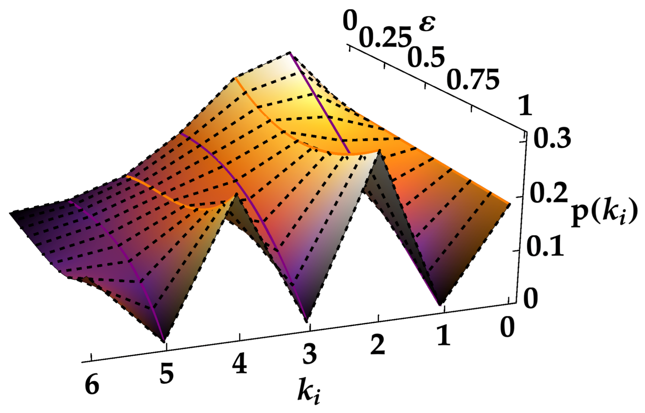
3.1. The Effects of the OCT on the Photon-Number Statistics of the TWB

Here we exploit the model developed in Section 2.1 to investigate the effects of the OCT on the detection of light and, in particular, on the statistics of a multi-mode mesoscopic TWB. The topic has been already widely investigated [13,14,16,17,19]. Still, we are anyway going through this point in order to test our model and use it to provide new insights on the OCT effects implied by this description.
From the inspection of Equation (8), we find that the joint probability of detecting k i events on the idler and k s on the signal is given by
P ( k s , k i ) = ( 1 λ 2 ) μ ε 1 ε k s + k i m s = k s 2 k s m i = k i 2 k i m s k s m s m i k i m i ( 1 ε ) 2 ε η 1 η m s + m i n = max ( m s , m i ) n + μ 1 n n m s n m i λ ( 1 η ) 2 n
which is the extension of the joint probability retrieved in [4], where just the effect of a limited quantum efficiency is considered.
If we consider the marginal distribution from Equation (16) for the idler beam, we find
p ( k i ) = ( 1 λ 2 ) μ ( ( 1 ε ) η λ 2 ) k i ( 1 λ 2 ( 1 η ) ) k i + μ l = 0 k i 2 k i + μ 1 l μ 1 k i l l 1 λ 2 ( 1 η ) ( 1 ε ) 2 η λ 2 ε l = ( 1 λ 2 ) μ ( ( 1 ε ) η λ 2 ) k i ( 1 λ 2 ( 1 η ) ) k i + μ k i + μ 1 μ 1 · 2 F 1 k i 1 2 , k i 2 ; ( k i + μ 1 ) ; 4 ε 1 λ 2 ( 1 η ) ( 1 ε ) 2 η λ 2
where · is the floor function and 2 F 1 ( a , b ; c ; x ) is the ordinary hypergeometric function. It can be shown that Equation (17) can be obtained from Equation (9) as well by replacing P n with the photon-number distribution of a multi-mode TWB state [6,24]. We also remark that, as we showed in [21], in the single-mode case (i.e., μ = 1 ) Equation (17) reduces to a linear combination of Fibonacci polynomials, which should be kept in mind for the considerations that follow.
As a first remark, we stress that our model for the OCT, as outlined in Section 2.1, accounts for first-order events only. In the following paragraph, we briefly explore the implications of our simplified model for arbitrary values of ε . Then we move back to the realistic case related to our experiment.
We show the transformation of the detected-photon number statistics of TWBs due to the OCT in Figure 2 for the single-mode case and in Figure 3 for the multi-mode one. In both figures, we set the quantum efficiency η = 0.17 and the mean photon number N = 10 (see Equation (2)), which are experimentally reasonable values as long as SiPMs are employed for detection (see Section 4) and the photon-number regime is mesoscopic (see Section 2). For what concerns the multi-mode case, we have considered the limit μ , since, again, this case is comparable with the number of modes estimated in our experiments, where μ 2000 [17]. As μ , the multi-thermal distribution of TWB converges to a Poissonian one, whereas the detected-event distribution in Equation (17) tends to
p μ ( k i ) = exp k ^ i 1 + ε l = 0 k i 2 k i l l 1 ( k i l ) ! ε 1 ε l 1 ε 1 + ε k ^ i k i l .
Note that here we replaced the parameter λ with k ^ i through Equation (10).
At a first glance to Figure 2, we note that the OCT gives rise to an asymmetry in the detected-event distribution: the detection probability of even events enhances proportionally to ε as the detection probability of odd events declines. Moreover, this effect is smoothed as the detected-event k i increases. A further inspection of our OCT model may help to understand why. Let m be the number of photons detected with probability η . As mentioned above, according to our OCT model, the outcome is a number k such that m k 2 m . If m is odd, then m / 2 of the possible values for k are odd and m / 2 are even, but, if m is even, ( m + 1 ) / 2 of the possible values for k are even while still just m / 2 are odd. This is basically due to the fact that 2 m , the superior bound to k, is always even. However, as m increases, such a difference between even and odd detected-photon numbers becomes negligible compared to k. This effect is especially apparent if we look at Equation (17) in the single-mode case. As mentioned above, in such a situation the detected-event distribution reduces to a linear combination of Fibonacci polynomials. This family of polynomials can be defined as [31]
F n ( x ) 1 2 n x 2 + 4 + x n + ( 1 ) n + 1 x 2 + 4 x n x 2 + 4
for given n N . The index of the polynomials in the single-mode detected-event distribution is n = k i + 1 , so that we get larger contributions as k i is even and smaller otherwise.
In Figure 4 and Figure 5 we emphasize the most obvious effect of the OCT on the statistics of detected photons, i.e., compared to the case where no OCT affects the measurement, the probability of detecting smaller numbers of events is depleted, while, on the contrary, the larger values of k are more likely to be revealed. An expected effect of the OCT which, rather than a consequence, is the very definition of it. Note that here we focus on experimental values of ε , which are typically small ( ε < 0.1 ) due to the recent technological improvements mentioned above. The plots show the ratio between the difference Δ p p ( k i ) p 0 and p 0 , where p 0 p ( k i ) | ε = 0 . Again, we explore the single-mode case in Figure 4, and the multi-mode limit case in Figure 5, having fixed every parameter as before. Note that the effect of the OCT in the two cases is the same, as the differences between the two plots have to be ascribed uniquely to the different distributions of pure photons, single-thermal in Figure 4 and Poissonian in Figure 5.

3.2. The Effects of the OCT on the Photon-Number Statistics of the Conditional State

Here we investigate the effects of the OCT on the statistics of the signal after conditioning over the idler, as described in Section 2.1. We also consider the effect of the imbalance between the quantum efficiencies of the signal and idler detectors.
Note that, while we remove the assumption that the detectors of the two parties share the same quantum efficiency η = η s = η i , we keep assuming the same OCT probability ε = ε s = ε i . The imbalance is introduced through the parameter α η s / η i , with η η i .
The expression of the reduced state of the signal after measuring k i events over the idler is straightforward from Equation (11) and reads
ρ ^ s ( k i ) = ( 1 λ 2 ) μ p ( k i ) ε 1 ε k i m i = k i 2 k i m i k i m i ( 1 ε ) 2 ε η 1 η m i j = 1 μ l j δ m i , γ n j = l j n j m j λ 2 n j ( 1 η ) n j | n j n j |
where again γ j = 1 μ l j and · is the ceiling function. Note that the conditional state correctly does not depend on α since no detection over the signal party has occurred yet.
On the contrary, the related detected-event distribution is a function of α , other than of the number of events detected over the idler k i :
p ( k i ) ( k s ) = ( 1 λ 2 ) μ p ( k i ) ε 1 ε k i + k s m i = k i 2 k i m s = k s 2 k s m i k i m i m s k s m s ( 1 ε ) 2 ε η 1 η m i ( 1 ε ) 2 ε α η 1 α η m s l = m s l + μ 1 l l m s l m i λ 2 l ( 1 η ) l ( 1 α η ) l .
In the limit of large number of modes, we find
p μ ( k i ) ( k s ) = exp k i η ( 1 + ε ) p μ ( k i ) ε 1 ε k i + k s m i = k i 2 k i m s = k s 2 k s m i k i m i m s k s m s ( 1 ε ) 2 ε η 1 η m i ( 1 ε ) 2 ε α η 1 α η m s l = m s 1 l ! l m s l m i k i ( 1 η ) ( 1 α η ) η ( 1 + ε ) l .
Given Equation (21), we can have access to every moment of the conditional-state distribution. For instance, the first moment reads
k ^ s ( k i ) = α η ( 1 + ε ) 1 λ 2 ( 1 η ) k i + μ λ 2 ( 1 η ) x log χ ( x ) | x = 0
where
χ ( x ) l = 0 k i 2 k i + μ 1 l μ 1 k i l l 1 λ 2 ( 1 η ) ( 1 ε ) 2 η λ 2 ε l e l x
is a sort of characteristic function related to the discrete probability distribution in Equation (17). Indeed, one can easily prove that Equation (17) can be rewritten as
p ( k i ) = ( 1 λ 2 ) μ [ ( 1 ε ) η λ 2 ] k i [ 1 λ 2 ( 1 η ) ] k i + μ χ ( 0 ) .
The logarithmic derivatives of χ ( x ) evaluated in x = 0 contribute to the moments of the conditional state, as shown in Equation (23) for the mean value. If ε is set to 0 and α to 1 in Equation (23), we retrieve the result reported in [4] for the limited-quantum-efficiency condition, i.e.,
k ^ s ( k i ) ( ε = 0 , α = 1 ) = k i ( k ^ i + η μ ) + μ k ^ i ( 1 η ) k ^ i + μ .

3.3. The Effects of the OCT on the Nonclassicality of the Conditional State

Finally, we focus on the nonclassicality of the state generated after post-selection and evaluate to what extent the OCT is detrimental for this quantum resource.
The first and the second moments of the conditional-state distribution allow us to retrieve the Fano factor for the detected events by means of Equation (14) expressed for the operator k ^ s . As mentioned in Section 2.1, the Fano factor provides a sufficient condition for nonclassicality. For the distribution of the conditional state in Equation (21) we find that it reads
F s ( k i ) = 1 + 3 ε 1 + ε α η ( 1 + ε ) + 1 k ^ s ( k i ) α η ( 1 + ε ) 1 λ 2 ( 1 η ) 2 λ 2 ( 1 η ) ( k i + μ ) 1 k ^ s ( k i ) α η ( 1 + ε ) 1 λ 2 ( 1 η ) 2 · x log χ ( x ) λ 2 ( 1 η ) x log x log χ ( x ) | x = 0
where χ ( x ) is defined in Equation (24). Again, we highlight that Equation (27) can be written as a function of experimental quantities by just replacing λ with k i through Equation (10). Since the expression is quite complex, in Figure 6 we show the behavior of F s ( k i ) as a function of the conditioning value k i for different choices of the other parameters: in panel (a), different mean values of the unconditioned state k i , in panel (b), different values of the balance parameter α , in panel (c), different choices of the cross-talk probability ε , and finally in panel (d), different number of modes of the unconditioned state μ . It is worth noting that the subPoissonianity of the Fano factor can be increased by decreasing the mean value of the unconditioned state and increasing the number of modes, and by operating on the features of the detectors, namely reducing the OCT probability and increasing the balance factor.
Again, if ε = 0 and α = 1 , we retrieve the known expression of the Fano factor for the conditional state in the context of multi-mode TWB states and limited quantum efficiency, as outlined in [6], i.e.,
F s ( k i ) ( ε = 0 , α = 1 ) = ( 1 η ) 1 + k ^ i ( k i + μ ) ( k ^ i + η μ ) ( k ^ i + μ ) [ ( k i + μ ) ( k ^ i + η μ ) η μ ( k ^ i + μ ) ] .
Note that Equation (27) can be significantly simplified by taking the limit to realistic values for the parameters μ and ε . As mentioned above, our experimental conditions allow us to take the limit μ , which reduces the sum in Equation (24) to
χ ( 0 ) k i 1 ε 1 + ε k i l = 0 k i 2 1 l ! ( k i 2 l ) ! ε ( 1 + ε ) k ^ i ( 1 ε ) 2 l ,
but then, being the typical OCT probabilities of modern SiPMs of the order 10 2 , the largest order in the argument of the sum for a given term l is
( ε / k ^ i ) l l ! ( k i 2 l ) ! .
Thus, provided that the order of the mean number of detected events is larger than the order of ε , the argument of the sum gets smaller as l increases. If we keep the l = 0 term only, all the logarithmic derivatives of χ ( x ) are null, so that the mean value and the Fano factor of the conditional state are much simplified. By taking this limit, we neglect the OCT contribution provided by the asymmetry between odd and even detected events, which is reasonable if ε is small (i.e., ε < 0.1 ), as highlighted in Figure 4 and Figure 5. Given this approximation and the limit for μ , one gets
k ^ s μ ( k i ) = α [ η ( 1 + ε ) k i + ( 1 η ) k ^ i ] F s μ ( k i ) = 1 + 3 ε 1 + ε α η ( 1 + ε ) 1 ( 1 η ) k ^ i η ( 1 + ε ) k i + ( 1 η ) k ^ i .
Equations (31) allow us to find the threshold conditioning value k ¯ such that the detected state is nonclassical, i.e., F s μ ( k i < k ¯ ) < 1 . Before retrieving k ¯ , we remark that in the limit μ , the Fano factor in Equation (28), where ε = 0 and α = 1 , is a function of the quantum efficiency only, i.e.,
F s μ ( k i ) ( ε = 0 , α = 1 ) = 1 η 1 η / 2 .
However, 0 F s μ ( k i ) ( ε = 0 , α = 1 ) 1 η [ 0 , 1 ] , which means that the imperfections in detection due to limited quantum efficiency never provide a detected superPoissonian statistics in this context. Only in the limit case η = 0 the nonclassicality of a conditional state from multi-mode TWB is not revealed by the Fano factor, otherwise the detected nonclassicality is just reduced with respect to the ideal case ( η = 1 ). On the contrary, the OCT can completely conceal the quantum nature of a conditional state since we may have F s μ ( k i ) > 1 for some k i < k ¯ where
k ¯ = 2 ε ( 1 η ) k ^ i η ( 1 + ε ) [ α η ( 1 + ε ) 2 2 ε ] .
Note that k ¯ > 0 α η ( 1 + ε ) 2 > 2 ε , i.e., if
η s > η t h ( ε ) 2 ε ( 1 + ε ) 2
where we replaced α η with the quantum efficiency of the detector of the signal party η s through the definition of α . Therefore, Equation (33) shows that for ε > 0 and η < 1 there is a conditioning number k ¯ > 0 such that if k i < k ¯ the detected statistics is superPoissonian (see Figure 6). Moreover, Equation (34) gives an experimental condition for the observation of the nonclassicality of the conditional state: provided that η s is larger than the threshold η t h , then a finite k ¯ exists such that one can measure F s μ ( k i ) < 1 k i > k ¯ . Note that k ¯ ( ε = 0 , η 0 ) = 0 , which implies that the detected statistics is subPoissonian, if the only detection imperfection is a non-unit η > 0 . However, it is remarkable that in the ideal case η = 1 we have a subPoissonian statistics independently of ε , while if η 0 and ε 0 , then the detected statistics is always superPoissonian, independently of k i .
One may ask if a combination of η and ε exists such that F s μ ( k i ) = 0 for some k i . Unfortunately, this is not the case since in the second line of Equations (31) the Fano factor is a monotone decreasing function of k i and it converges to an asymptotic value which is strictly positive ε > 0 . Finally, we remark that the threshold in Equation (34) is directly connected to the sub-Poissonianity of the original state, which in turn depends on its intrinsic nonclassical correlations. In fact the same threshold can be shown to hold for the observation of sub-shot-noise correlations of TWB. The sub-Poissonianity condition on correlations can be expressed by the noise reduction factor as R < 1 , where R is defined as the ratio of the variance of the difference of detected events and the mean value of their sum, i.e.,
R Δ ( k ^ s k ^ i ) 2 k ^ s + k ^ i .
We showed in Ref. [20] that, in the case of TWB states with a large number of modes, this figure of merit can be reduced to
R = 1 α η ( 1 + ε ) + 2 ε 1 + ε ,
which gives R < 1 for the same condition as in Equation (34). Hence, the connection between the sub-Poissonianity condition and the requirement on the quantum efficiency in Equation (34) is straightforward. Incidentally, note that the Fano factor in the second of Equations (31) can be expressed in terms of the noise reduction factor.

4. Discussion

In order to validate the model for conditioning addressed in the previous Section, hereafter we present and discuss the experimental generation of nonclassical conditional states. As already explained in [6,17,18], such states can be obtained in post-processing by selecting a certain number of photons in one TWB arm and reconstructing the modified distribution of photons in the other arm. In Section 3 we showed that the unconditioned state is formally described by a multi-thermal distribution, which reduces to Equation (18) when the light in one arm is characterized by a very large number of modes [32,33,34] and is detected by a SiPM characterized by an OCT probability ε 0 . In Figure 7 we show the detected-event distributions having mean values k = 2.63 (panel (a)), 2.66 (panel (b)), 1.43 (panel (c)), and 0.57 (panel (d)). The experimental data are shown as gray dots, while the theoretical fitting functions according to Equation (18) are presented as gray lines. To quantify the agreement between the experimental data and the theoretical expectations we evaluate the fidelity f = m = 0 m ¯ P th ( k ) P ( k ) , in which P th ( k ) and P ( k ) are the theoretical and experimental distributions, respectively, and the sum extends up to the maximum number of detected events k above which both P th ( k ) and P ( k ) become negligible.
From the fitting procedure, it is possible to obtain the value of the only fitting parameter, namely the OCT. In particular, we notice that for the four considered measurements, the OCT value is of the same order of magnitude and always less than 1%, thus proving that the cross-talk probability affecting this model of SiPM is really small, even if not completely negligible. We remark that the estimated values for the OCT probability in Figure 8 are smaller than those reported in the datasheet of our sensors [30], but consistent with the characterization that we have already provided for these SiPMs in [16].
In order to prove that the conditioning procedure changes the statistical properties of such states making them sub-Poissonian, we calculate the Fano factor of the conditional states obtained from each of the four considered unconditioned states. Indeed, as mentioned in Section 2.1, F < 1 is a sufficient condition for nonclassicality.
In Figure 8 we show the experimental Fano factors shown as dots plus error bars, while the theoretical fitting functions according to the second line of Equations (31) are shown as dashed lines with the same color choice. For all the fitting functions we left η and α as free fitting parameters, while we used the same values of ε obtained from the fitting of the marginal distributions. In particular, in all cases we obtained a balance factor α 0.99 and a quantum efficiency η 0.14 . As a general statement, we note that the data corresponding to the conditioning value k i = 1 are larger than 1 for the largest mean values. Such a behavior is in agreement with the theoretical expectation expressed by the second line of Equations (31) and the plots in panel (a) of Figure 6. Moreover, we emphasize that for the smallest mean value the conditioning operation is applied up to k i = 3 because the number of experimental data is not sufficient to reliably build the states corresponding to k i > 3 .
In order to explore in which way the conditional measurements modify the statistical properties of the unconditioned states in the presence of the OCT, in the two panels of Figure 9 we show some conditional distributions at different conditioning values together with the corresponding unconditioned statistics having mean values k = 2.66 (panel (a)), and 1.43 (panel (b)). The data are presented as colored dots plus error bars ( k i = 1 in black, k i = 2 in red, and k i = 3 in blue), while the theoretical expectations are shown as solid lines with the same color choice. The theoretical curves have been calculated according to Equation (22) using the parameter values of ε obtained from the fit of the unconditioned states (see caption of Figure 7) and those of η and α obtained from the fit of the Fano (see caption of Figure 8). For the sake of clarity, in each panel of Figure 9 we show again the statistics of the unconditioned state as gray dots and the theoretical expectation as gray surface defined by dashed line. As expected from the two panels of the figure, it clearly appears that the conditional measurements change the statistics of the input state. Even in this case, to quantify the agreement between the experimental data and the theoretical expectations we evaluate the fidelity. We note that the higher the conditioning value the lower the fidelity value. This fact can be ascribed to the limited number of data at our disposal to build the statistics, which is lower and lower at increasing values of k i . Larger acquisitions of data could overcome such a limit. At the same time, the good dynamic range of SiPMs would suggest that both the unconditioned states and the corresponding conditional ones could be more populated, thus allowing us to really explore the mesoscopic intensity domain.
In general, the good agreement between the experimental data and the theoretical expectations validate the model used to describe the role played by the non-idealities of the employed detectors, namely the cross-talk effect, the non-unitary quantum efficiency and the possible imbalance between the two quantum efficiencies. We emphasize that the detection of subPoissonian states was achieved because, even in the presence of a limited quantum efficiency, the OCT probability is small enough to ensure that η > η t h . This is not the case of either previous sensors generations, in which the OCT probability was more than 10 % , or new kinds of SiPMs with a higher sensitivity in the near infrared region. Indeed, the best generation of such detectors exhibits a cross talk probability of 6% and a low quantum efficiency (less than 20%), which could prevent the generation of nonclassical states by conditional measurements.

5. Conclusions

In this paper we addressed a thorough theoretical model for the conditional measurements with SiPMs. In particular, we included the contribution of the OCT and we took into account the possibility of an imbalance between the two detection chains. We provided a complete description of the detection of a multi-mode TWB state in the presence of the OCT, showing explicitly the effects of such correlated noise on the reconstructed distribution. We obtained a closed formula for the detected-event distribution of the conditional states and an analytic expression for the first moments. Hence, we retrieved the Fano factor, which represents a sufficient criterion for nonclassicality. In particular, we found that, in the presence of cross-talk effect, nonclassicality is more easily attained by:
-
reducing the imbalance between the two detection arms;
-
decreasing the mean value of the unconditioned states;
-
increasing the number of modes.
Moreover, we found a useful bound between the quantum efficiency of the detectors and the OCT probability, which sets a link between their mutual values for still revealing the nonclassicality of conditional states. Actually, we demonstrated that this bound is valid in general for the twin-beam states, on which the conditioning operation is performed.
The theoretical expectations have been validated by the experimental generation of conditional states by conditional measurements performed on multi-mode TWB states with SiPMs. The good agreement between the experimental data and the theoretical predictions suggests that the conditional measurements can be performed even on more populated states to produce well-populated conditional states as well by exploiting the good dynamic range of SiPMs.
Finally, we hint that the model may be further improved by including the dark counts, which is another common drawback of SiPMs at room temperature. However, it is worth noting that in the case of a light signal integrated over short gate widths [17], which correspond to our experimental condition, the mean number of dark counts is remarkably low, which is the reason why we did not address this topic here. Moreover, it could be interesting to include cascade effects and generation of multiple secondary avalanches in the model for the OCT, so that a realistic case for large ε could be compared with the one explored here.

Author Contributions

G.C., A.A. and M.B. conceptualized the work, G.C. performed the theoretical calculations, G.C. and A.A. performed the measurements, A.A. and M.B. analysed and interpreted the data, G.C. and A.A. drafted the work, M.B. substantively revised it. All authors have read and agreed to the published version of the manuscript.

Funding

This research received no external funding.

Institutional Review Board Statement

Not applicable.

Informed Consent Statement

Not applicable.

Data Availability Statement

The datasets used and analysed during the current study are available from the corresponding author on reasonable request.

Conflicts of Interest

The authors declare no conflict of interest.

Abbreviations

The following abbreviations are used in this manuscript:
PNRPhoton Number Resolving
SiPMSilicon Photomultiplier
OCTOptical Cross-Talk
TWBTwin Beam
POVMPositive Operator-Valued Measure

References

  1. Paris, M.G.A. The modern tools of quantum mechanics. Eur. Phys. J. Spec. Top. 2012, 203, 61–86. [Google Scholar] [CrossRef]
  2. Ben-Zion, D.; McGreevy, J.; Grover, T. Disentangling quantum matter with measurements. Phys. Rev. B 2020, 101, 115131. [Google Scholar] [CrossRef] [Green Version]
  3. Paris, M.G.A.; Cola, M.; Bonifacio, R. Quantum-state engineering assisted by entanglement. Phys. Rev. A 2003, 67, 042104. [Google Scholar] [CrossRef] [Green Version]
  4. Allevi, A.; Andreoni, A.; Beduini, F.A.; Bondani, M.; Genoni, M.G.; Olivares, S.; Paris, M.G.A. Conditional measurements on multimode pairwise entangled states from spontaneous parametric downconversion. EPL 2010, 92, 20007. [Google Scholar] [CrossRef]
  5. Allevi, A.; Andreoni, A.; Bondani, M.; Genoni, M.G.; Olivares, S. Reliable source of conditional states from single-mode pulsed thermal fields by multiple-photon subtraction. Phys. Rev. A 2010, 82, 013816. [Google Scholar] [CrossRef] [Green Version]
  6. Lamperti, M.; Allevi, A.; Bondani, M.; Machulka, R.; Michálek, V.; Haderka, O.; Peřina, J., Jr. Optimal sub-Poissonian light generation from twin beams by photon-number resolving detectors. J. Opt. Soc. Am. B 2014, 31, 20–25. [Google Scholar] [CrossRef] [Green Version]
  7. Peřina, J., Jr.; Haderka, O.; Michálek, V. Simultaneous observation of higher-order non-classicalities based on experimental photocount moments and probabilities. Sci. Rep. 2019, 9, 1–8. [Google Scholar] [CrossRef]
  8. Dakna, M.; Anhut, T.; Opatrný, T.; Knöll, L.; Welsch, D.G. Generating Schrödinger-cat-like states by means of conditional measurements on a beam splitter. Phys. Rev. A 1997, 55, 3184. [Google Scholar] [CrossRef] [Green Version]
  9. Olivares, S.; Paris, M.G.A.; Bonifacio, R. Teleportation improvement by inconclusive photon subtraction. Phys. Rev. A 2003, 67, 032314. [Google Scholar] [CrossRef] [Green Version]
  10. Cerf, N.J.; Krüger, O.; Navez, P.; Werner, R.F.; Wolf, M.M. Non-Gaussian Cloning of Quantum Coherent States is Optimal. Phys. Rev. Let. 2005, 95, 070501. [Google Scholar] [CrossRef] [Green Version]
  11. Eisert, J.; Scheel, S.; Plenio, M.B. Distilling Gaussian States with Gaussian Operations is Impossible. Phys. Rev. Lett. 2002, 89, 137903. [Google Scholar] [CrossRef]
  12. Caccia, M.; Chmill, V.; Ebolese, A.; Locatelli, M.; Martemiyanov, A.; Pieracci, M.; Risigo, F.; Santoro, R.; Tintori, C. An Educational Kit Based on a Modular Silicon Photomultiplier System. In Proceedings of the 2013 3rd International Conference on Advancements in Nuclear Instrumentation, Measurement Methods and Their Applications (ANIMMA), Marseille, France, 23–27 June 2013; Volume 978, pp. 1–7. [Google Scholar]
  13. Afek, I.; Natan, A.; Ambar, O.; Silberberg, Y. Quantum state measurements using multipixel photon detectors. Phys. Rev. A 2009, 79, 043830. [Google Scholar] [CrossRef] [Green Version]
  14. Ramilli, M.; Allevi, A.; Chmill, V.; Bondani, M.; Caccia, M.; Andreoni, A. Photon-number statistics with silicon photomultipliers. J. Opt. Soc. Am. B 2010, 27, 852–862. [Google Scholar] [CrossRef] [Green Version]
  15. Kalashnikov, D.A.; Tan, S.H.; Iskhakov, T.S.; Chekhova, M.V.; Krivitsky, L.A. Measurement of two-mode squeezing with photon number resolving multipixel detectors. Opt. Lett. 2012, 37, 2829–2831. [Google Scholar] [CrossRef] [PubMed] [Green Version]
  16. Chesi, G.; Malinverno, L.; Allevi, A.; Santoro, R.; Caccia, M.; Martemiyanov, A.; Bondani, M. Optimizing Silicon Photomultipliers for Quantum Optics. Sci. Rep. 2019, 9, 1–12. [Google Scholar] [CrossRef] [PubMed]
  17. Chesi, G.; Malinverno, L.; Allevi, A.; Santoro, R.; Caccia, M.; Bondani, M. Measuring nonclassicality with silicon photomultipliers. Opt. Lett. 2019, 44, 1371–1374. [Google Scholar] [CrossRef] [PubMed] [Green Version]
  18. Chesi, G.; Allevi, A.; Bondani, M. Autocorrelation functions: A useful tool for both state and detector characterisation. Quantum Meas. Quantum Metrol. 2019, 6, 1–6. [Google Scholar] [CrossRef]
  19. Nagy, F.; Mazzillo, M.; Renna, L.; Valvo, G.; Sanfilippo, D.; Carbone, B.; Piana, A.; Fallica, G.; Molnar, J. Afterpulse and delayed crosstalk analysis on a STMicroelectronics silicon photomultiplier. Nucl. Instrum. Methods Phys. Res. A 2014, 759, 44–49. [Google Scholar] [CrossRef]
  20. Chesi, G.; Allevi, A.; Bondani, M. Effects of nonideal features of silicon photomultiplier on the measurements of quantum correlations. Int. J. Quantum Inf. 2019, 17, 1941012. [Google Scholar] [CrossRef]
  21. Chesi, G.; Allevi, A.; Bondani, M. Effect of cross-talk on conditional measurements performed with multi-pixel photon counters. In Proceedings of the 2020 IMEKO TC-4 International Symposium, Palermo, Italy, 14–16 September 2020. [Google Scholar]
  22. Couteau, C. Spontaneous parametric down-conversion. Contemp. Phys. 2018, 59, 291–304. [Google Scholar] [CrossRef] [Green Version]
  23. Paleari, F.; Andreoni, A.; Zambra, G.; Bondani, M. Thermal photon statistics in spontaneous parametric downconversion. Opt. Lett. 2004, 12, 2816–2824. [Google Scholar] [CrossRef] [Green Version]
  24. Allevi, A.; Olivares, S.; Bondani, M. Measuring high-order photon-number correlations in experiments with multimode pulsed quantum states. Phys. Rev. A 2012, 85, 063835. [Google Scholar] [CrossRef] [Green Version]
  25. Van Dam, H.T.; Seifert, S.; Vinke, R.; Dendooven, P.; Löhner, H.; Beekman, F.J.; Schaart, D.R. A Comprehensive Model of the Response of Silicon Photomultipliers. IEEE Trans. Nucl. Sci. 2010, 57, 2254–2266. [Google Scholar] [CrossRef] [Green Version]
  26. Vinogradov, S. Analytical models of probability distribution and excess noise factor of solid sate photomultiplier signals with crosstalk. Nucl. Instruments Methods Phys. Res. Sect. A Accel. Spectrometers Detect. Assoc. Equipment 2012, 695, 247–251. [Google Scholar] [CrossRef] [Green Version]
  27. Gallego, L.; Rosado, J.; Blanco, F.; Arqueros, F. Modeling crosstalk in silicon photomultipliers. J. Instrum. 2013, 8, P05010. [Google Scholar] [CrossRef] [Green Version]
  28. Glauber, R.J. The Quantum Theory of Optical Coherence. Phys. Rev. 1963, 130, 2529–2539. [Google Scholar] [CrossRef] [Green Version]
  29. Klyshko, D.N. The nonclassical light. Phys.-Usp. 1996, 39, 573–596. [Google Scholar] [CrossRef]
  30. MPPC S13360-1350CS. Available online: http://www.hamamatsu.com/us/en/S13360-1350CS.html (accessed on 17 May 2021).
  31. Bicknell, M. A primer for the Fibonacci numbers VII. Fibonacci Quart. 1970, 8, 407–420. [Google Scholar]
  32. Allevi, A.; Lamperti, M.; Bondani, M.; Peřina, J., Jr.; Michálek, V.; Haderka, O.; Machulka, R. Characterizing the nonclassicality of mesoscopic optical twin-beam states. Phys. Rev. A 2013, 88, 063807. [Google Scholar] [CrossRef] [Green Version]
  33. Machulka, R.; Haderka, O.; Peřina, J., Jr.; Lamperti, M.; Allevi, A.; Bondani, M. Spatial properties of twin-beam correlations at low- to high-intensity transition. Opt. Express 2014, 22, 13374–13379. [Google Scholar] [CrossRef] [PubMed] [Green Version]
  34. Allevi, A.; Bondani, M. Statistics of twin-beam states by photon-number resolving detectors up to pump depletion. J. Opt. Soc. Am. B 2014, 31, B14–B19. [Google Scholar] [CrossRef]
Figure 1. Setup of the experiment described in [17] and addressed in Section 4 to provide experimental evidence to the model presented here. See the text for details.
Applsci 11 04579 g001
Figure 2. Detected-event distribution of the idler beam from Equation (17) in the single-mode case ( μ = 1 ) as a function of the number of detected events k i and of the OCT probability ε . We set the quantum efficiency η to 0.17 , while the mean photon number N to 10. These choices, together with a selected value of ε , yield the corresponding mean value k i = ( 1 + ε ) η N . The plot shows the evolution of a single-thermal distribution due to the OCT.
Applsci 11 04579 g002
Figure 3. Detected-event distribution of the idler beam from Equation (18) in the multi-mode limit case ( μ ) as a function of the number of detected events k i and of the OCT probability ε . We set the quantum efficiency η to 0.17 , while the mean photon number N to 10. These choices, together with a selected value of ε , yield the corresponding mean value k i = ( 1 + ε ) η N . The plot shows the evolution of a Poissonian distribution due to the OCT.
Applsci 11 04579 g003
Figure 4. Plots of the relative differences Δ p / p 0 , with Δ p = p ( k i ) p 0 and p 0 p ( k i ) | ε = 0 , in the single-mode case ( μ = 1 ) as a function of the number of detected events k i , for different values of the OCT probability ε , which are ε = 1 % (green), ε = 3 % (red), ε = 5 % (blue), ε = 7 % (grey) and ε = 9 % (violet). The quantum efficiency η and the mean photon number N are again set to 0.17 and 10, respectively.
Applsci 11 04579 g004
Figure 5. Plots of the relative differences Δ p / p 0 , with Δ p = p ( k i ) p 0 and p 0 p ( k i ) | ε = 0 , in the multi-mode limit case ( μ ) as a function of the number of detected events k i , for different values of the OCT probability ε , which are ε = 1 % (green), ε = 3 % (red), ε = 5 % (blue), ε = 7 % (grey) and ε = 9 % (violet). The quantum efficiency η and the mean photon number N are again set to 0.17 and 10, respectively.
Applsci 11 04579 g005
Figure 6. Fano factor of the conditional states as a function of the conditioning values for different choices of the other parameters involved in Equation (27). Panel (a): F for different choices of the mean value of the unconditioned state. From bottom to top: k = 0.5 (black), k = 1 (red), k = 1.5 (blue), k = 2 (green), k = 2.5 (magenta), k = 3 (cyan). The other parameters are: η = 0.17 , μ = 100 , α = 1 , and ε = 0.01 . Panel (b): F for different choices of the balance factor. From top to bottom: α = 0.5 (black), α = 0.6 (red), α = 0.7 (blue), α = 0.8 (green), α = 0.9 (magenta), α = 1 (cyan). The other parameters are: η = 0.17 , μ = 100 , k = 2 , and ε = 0.01 . Panel (c): F for different choices of the cross-talk probability. From bottom to top: ε = 0.01 (black), ε = 0.02 (red), ε = 0.05 (blue), ε = 0.10 (green), ε = 0.15 (magenta), ε = 0.20 (cyan). The other parameters are: η = 0.17 , μ = 100 , k = 2 , and α = 1 . Panel (d): F for different choices of the number of modes of the unconditioned state. From top to bottom: μ = 1 (black), μ = 2 (red), μ = 5 (blue), μ = 10 (green), μ = 100 (magenta), μ = 1000 (cyan). The other parameters are: η = 0.17 , k = 2 , α = 1 , and ε = 0.01 .
Applsci 11 04579 g006
Figure 7. Detected-event distributions P ( k ) of the unconditioned state having mean value k = 2.63 (panel (a)), 2.66 (panel (b)), 1.43 (panel (c)), and 0.57 (panel (d)). The experimental data are shown as gray dots, while the theoretical expectations are presented as gray lines. The fidelity values are: f = 0.9999 in all panels.
Applsci 11 04579 g007
Figure 8. Fano factor as a function of the conditioning value for four different unconditioned states having mean values k = 2.63 (black), 2.66 (red), 1.43 (blue), and 0.57 (magenta). The experimental data are shown as dots plus error bars, while the theoretical fitting functions according to the second line of Equations (31) are presented as dashed curves with the same color choice. The fitting parameters are the following: η = 0.134 , α = 0.990 (black curve), η = 0.157 , α = 0.989 (red curve), η = 0.158 , α = 0.997 (blue curve), and η = 0.125 , α = 0.986 (magenta curve). The reduced χ ( 2 ) are: 0.34 (black curve), 0.14 (red curve), 0.94 (blue curve), and 0.05 (magenta curve).
Applsci 11 04579 g008
Figure 9. Detected-event distributions P ( k ) of the conditional states for k i = 1 (black curve), k i = 2 (red curve), and k i = 3 (blue curve) obtained from an unconditioned state having mean value k = 2.66 (panel (a)) and 1.43 (panel (b)). The experimental data are shown as colored symbols, while the theoretical expectations are presented as solid lines with the same color choice. The fidelity values are: f = 0.9999 , 0.9961, and 0.9888 in panel (a) and f = 0.9999 , 0.9954, and 0.9863 in panel (b). The unconditioned state is shown as gray dots and its theoretical expectation as gray surface defined by dashed line. The fidelity value is f = 0.9996 in panel (a) and f = 0.9999 in panel (b).
Applsci 11 04579 g009
Publisher’s Note: MDPI stays neutral with regard to jurisdictional claims in published maps and institutional affiliations.

