Multi-Step Traffic Speed Prediction Based on Ensemble Learning on an Urban Road Network

Abstract

Short-term traffic speed prediction plays an important role in the field of Intelligent Transportation Systems (ITS). Usually, traffic speed forecasting can be divided into single-step-ahead and multi-step-ahead. Compared with the single-step method, multi-step prediction can provide more future traffic condition to road traffic participants for guidance decision-making. This paper proposes a multi-step traffic speed forecasting by using ensemble learning model with traffic speed detrending algorithm. Firstly, the correlation analysis is conducted to determine the representative features by considering the spatial and temporal characteristics of traffic speed. Then, the traffic speed time series is split into a trend set and a residual set via a detrending algorithm. Thirdly, a multi-step residual prediction with direct strategy is formulated by the ensemble learning model of stacking integrating support vector machine (SVM), CATBOOST, and K-nearest neighbor (KNN). Finally, the forecasting traffic speed can be reached by adding predicted residual part to the trend one. In tests that used field data from Zhongshan, China, the experimental results indicate that the proposed model outperforms the benchmark ones like SVM, CATBOOST, KNN, and BAGGING.

1. Introduction

Various types of vehicles have pushed human society forward by making the mobility of people and goods possible, providing faster and more comfortable travel experience, facilitating social interactions, and so on. Nevertheless, the rapidly increasing number of vehicles has also brought some severe problems into worldwide cities. Apart from consequences like global warming and fossil fuel depletion, traffic congestion is one of the most negative effects that can be perceived by each traffic participant and it can inevitably result in a series of problems, such as traffic accidents, energy overconsumption, and significant travel delay [1]. In 2017, INRIX released the Urban Mobility Scorecard Annual Report, which showed that traffic congestion was a significant challenge in a large number of major cities around the world. According to this report, urban Americans spent a total of an extra 8.8 billion hours and purchased an extra 3.3 billion gallons of fuel because of congestion in 2017, giving a direct congestion cost of $166 billion [2]. Transportation and traffic researchers believe that the Intelligent Transportation Systems (ITS) is a promising solution to improve transportation management and can provide much better services that can eventually lead to less congestion than traditional methods [3,4]. Among such services, traffic prediction plays an important role in ITS because forecasting information can be utilized to support traffic guidance, signal optimization, and so on. For example, travelers can re-plan their traveling paths to avoid congestion and incidents, which could save their time and cost by using the forecasting information, such as traffic speed, travel time, and traffic condition [5]. Morever, accurate and timely speed prediction have also been key issues in traffic prediction horizon, even in the ITS horizon. Correspondingly, it has led to an intensive body of works about traffic speed prediction in the recent years. However, some major challenges about short-term traffic forecasting have been pointed out as follows [6,7]:

(1)

Traffic prediction based on spatial-temporal characteristics.

(2)

Further exploration of Artificial Intelligence (AI) in traffic flow prediction.

(3)

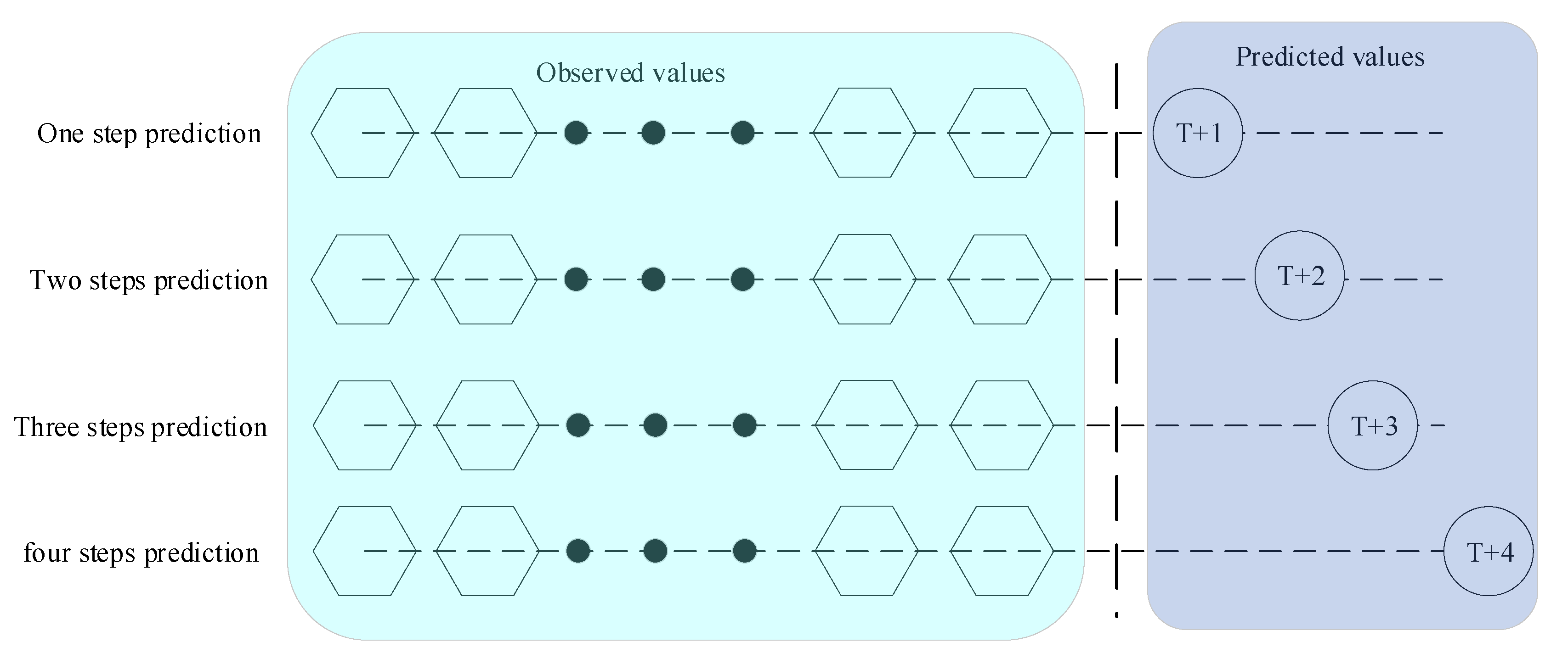
Multi-step prediction for real-life ITS applications to provide relatively long-term future traffic situation for road users and government.

Based on the aforementioned issues, a novel multi-step speed prediction model is proposed by considering spatial-temporal dependencies and using ensemble learning. The developed method separates original data into mean and residual time series, and then employs direct strategy and the ensemble learning framework of stacking algorithm to multi-step-ahead forecast the residual time series. Main contributions of this paper are listed as follows:

(1)

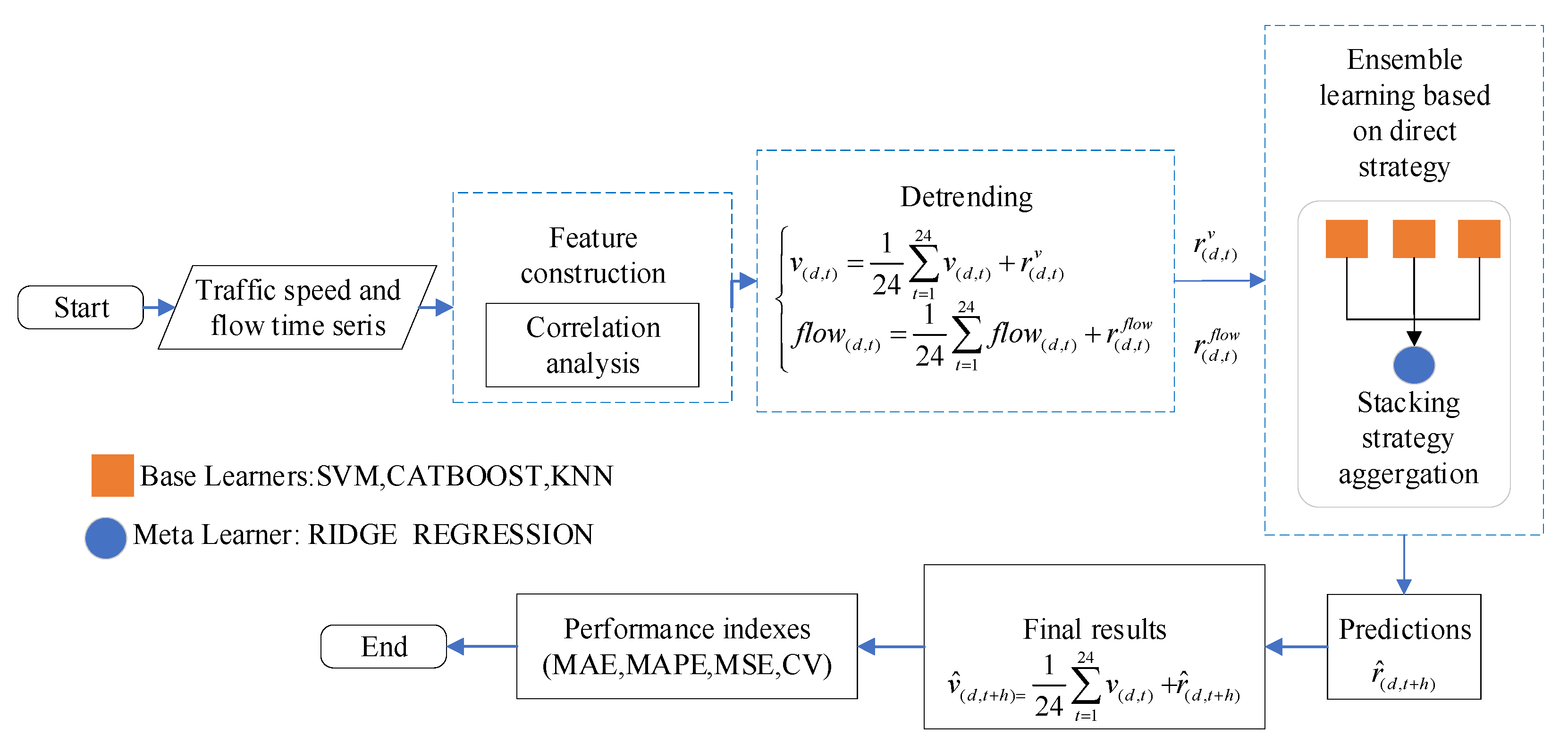
A novel multi-step prediction with detrending and direct strategy is achieved by the ensemble learning model of stacking (DDSELM) to forecast travel speed using spatial-temporal characteristics.

(2)

The proposed multi-step model is validated by using a very large field dataset of hourly average link traffic speed, which reveals it has good performance.

The remaining part of this paper is organized as follows: In Section 2, a summary of the state-of-the-art research in exploring traffic speed prediction is presented. Then, Section 3 formulates a new multi-step prediction model with ensemble learning. Subsequently, a field dataset of Zhongshan, China, is employed to validate the effectiveness of our model in Section 4 and Section 5, respectively. Finally, the conclusion and future work are presented in Section 6.

2. Related Work

In this section, a relevant background review about works on traffic speed prediction including parametric methods and non-parametric methods [8,9], machine learning, and multi-step prediction is provided.

Parametric methods, a well-structured family of models, estimate the model parameters based on the training data and have been widely used to conduct traffic forecast. For example, the auto-regressive integrated moving average (ARIMA) model was proposed in 1970s to predict short-term freeway traffic data [10]. Additionally, Voort et al. [11] proposed a KARIMA prediction model to forecast traffic flow, which combined Kohonen maps with ARIMA time series. Then, Williams et al. [12] provided a theoretical and empirical analysis of a seasonal ARIMA method, and Kumar et al. [13] extended it into the scenarios of the limited input data. In Kumar’s scheme, the prediction of the next day situation (24 h, start from the prediction moment) was only based on the historical data in the last three days. In 1984, Okutani et al. [14] applied Kalman filtering (KF) theory to traffic prediction and proved that KF could perform well in traffic prediction, and Guo et al. [15] introduced the adaptive KF approach to forecast stochastic short-term traffic flow. Along this line, Mir et al. [16] presented a KF model for travel speed prediction by minimizing the variance between the real-time speed measurement and its prediction. Zambrano-Martinez et al. [17] presented an intuitive formula to predict link travel time based on the degree of traffic congestion for route choice optimization.

Unlike the parametric methods, non-parametric ones have ability to flexibly capture the stochastic and nonlinear features of traffic state (i.e., speed, flow, occupancy, travel time). Vlahogianni et al. [8] pointed that traffic forecasting methods with computational intelligence (CI) have gradually replaced the traditional statistical ones, because they need no or little prior assumptions for input variables. As typical representatives, artificial neural networks (ANNs) have been successfully applied in many transportation domains [18,19]. ANNs are mathematical models that formulate information processing systems by imitating the structure and function of the neural network of the brain. For example, Vlahogianni et al. [20] proposed an advanced, genetic algorithm based multi-layered structural optimization strategy to predict traffic flow. Different from ANNs, Zhang et al. [21] proposed wavelet-based higher-order spatial-temporal (Wavelet-HST) method to accurately predict network-scale traffic speed with an improvement of 7.8%∼10.5% in the root mean square error than other six benchmark methods. Moreover, Cai et al. [22] improved the original KNN model based on spatiotemporal correlation for traffic prediction.

In recent years, with the rapid development of machine learning and deep learning techniques, more and more ITS researchers have begun to adopt these kinds of techniques for high-accuracy traffic prediction. As pointed out by Ma et al., the LSTM-NN can overcome the problem of back-propagated error decay by using memory blocks and has a better capability for time series prediction with long temporal dependency [23]. Additionally, a single-step support vector machine (SVM) with spatiotemporal parameters was proposed in 2017, which provided short-term traffic speed prediction results (5-min) with error ranging from 3.31% to 15.35% [24]. Moreover, Dong et al. [25] developed an extreme gradient boosting (XGBOOST) model with wavelets decomposition and reconstruction to predict the short-term traffic flow, which outperformed SVM.

Although single models are studied by many researchers and proved to be suitable for many cases, they still have some shortcomings [25]. Alternatively, it is a much better way to fuse the results from different prediction methods combined one to achieve better prediction accuracy than single predictor. For example, the ensemble learning models have been proved to achieve much better performance in prediction accuracy than individual ones [26]. Nowadays, ensemble learning has been used in many fields of traffic prediction, such as traffic sign detection and recognition [27], traffic speed [28], short-term traffic volume [29], and traffic incident detection [30].

However, current ensemble methods are not explicitly designed to deal with spatiotemporal data, and how to effectively ensemble multiple models while utilizing the spatiotemporal information remains a challenging, but practical, problem.

There is a tendency that more and more scholars draw their attentions on multi-step prediction. Usually, multi-step traffic prediction can provide drivers and traffic agencies more chances and time to pre-make better decisions than one-step prediction. Zhang et al. [31] reported a hybrid deep ensemble approach by integrating 3D convolutional neural network (CNN) with ensemble empirical mode decomposition (EEMD), and yielded the high performance regardless of prediction time step increases from 1 to 6. Notably, although the prediction time step increases, the evolving fuzzy neural network (EFNN) model with the consideration of the periodic pattern can also outperform other models (ANN, SVM, ARIMA, vector autoregressive model) with smaller prediction errors and slower raising rate of errors [5]. Zhang et al. [7] proposed a novel deep learning framework named attention graph convolutional sequence-to-sequence model (AGC-Seq2Seq) to accurately capture the temporal heterogeneity in multi-step traffic speed prediction. Papathanasopoulou et al. [32] embedded a microscopic traffic simulation of car-following model into dynamic multi-step traffic prediction and leaded to less than 10% error in speed prediction even for ten steps into the future.

3. Prediction Methodology

Previous studies show that ensemble learning can be used for traffic prediction with good performance. Thus, this paper will develop an ensemble learning model for multi-step traffic speed forecasting with direct strategy, namely DDSELM, to process the given time series data. Firstly, the correlation analysis is conducted to identify the key factors affecting speed forecasting. Then, a detrending algorithm is developed to divide the speed dataset into trend part (i.e., mean set) and residual one, and then this study employs direct strategy and ensemble learning of stacking to predict multi-step residuals. Finally, the multi-step residuals combined with the trend sets can form the final predict results.

3.1. Direct Strategy

The direct strategy was firstly proposed by Cox in 1961 in the fields of multi-step prediction. This strategy needs to establish a set of models for each step. Input variables of direct strategy depend on observed values instead of predicted ones [33,34]. For example, the framework of direction strategy is shown in Figure 1.

3.2. Feature Construction

Notably, representative features determine the performance of forecasting modeling. In order to determine the appropriate model inputs, this study chooses initially the ten spatiotemporal candidate variables of travel speed and flow for correlation analysis, as shown in

Table 1. Constructed feature candidates for the prediction model.

Representative Feature	Descriptions
v(d,t)	Speed at time t, day d
v(d−1,t)	Speed at time t, day d − 1
v(d−2,t)	Speed at time t, day d − 2
v(d−3,t)	Speed at time t, day d − 3
v(d−1,t+1)	Speed at time t + 1, day d − 1
v(d−2,t+1)	Speed at time t + 1, day d − 2
v(d−3,t+1)	Speed at time t + 1, day d − 3
v(u,t)	Upstream speed at time t, day d
v(d,t)	Downstream speed at time t, day d
flow(d,t)	Flow at time t, day d

, which involve the time of day, day of week, and upstream and downstream connected links. Correlation analysis is a statistical analysis method that studies the correlation between two or more random variables. Among them, the Pearson correlation coefficient proposed by Pearson in 1895 is one of the most influential coefficients in correlation analysis to select the final representative features for the prediction model [35].

3.3. Detrending

Since traffic speed time series used in this paper are different spatio-temporal characteristics (i.e., workdays or weekends, peak or off-peak hours), it is reasonable to split speed time series into its mean trends and residuals via detrending algorithm, and develop the model to predict the residual time series. Following the previous literature [36], a simple average method was used to find out the trend, which takes the average of daily traffic speed series into account in Equation (1). Among, the speed observation at the tth hour belonging to the dth day can be formulated as follows:

$$\{\begin{array}{c}{v}_{\left(d,t\right)}=\frac{1}{24}{\displaystyle {\displaystyle \sum }_{t=1}^{24}}{v}_{\left(d,t\right)}+r_{\left(d,t\right)}^v\\ flo{w}_{\left(d,t\right)}=\frac{1}{24}{\displaystyle {\displaystyle \sum }_{t=1}^{24}}flo{w}_{\left(d,t\right)}+r_{\left(d,t\right)}^{flow}\end{array}$$

(1)

where the first item on the right of the equation represents the average speed(flow) of the dth day; $r_{\left(d,t\right)}^v$ ($r_{\left(d,t\right)}^{flow}$) represents the speed(flow) residual at the tth hour on the dth day, which constitutes the speed(flow) residual time series. Next, a predicted model will be introduced to forecast the residuals.

3.4. Ensemble Learning

As aforementioned, the ensemble learning can perform well in dealing with regression and classification tasks. Bagging, boosting, and stacking are the three conventional ensemble learning algorithms to integrate weak models into a strong one for applications in different fields [37]. The final prediction of bagging algorithm is equal to the average of all base learners or underlying models. The common boost model is Adaboost. Boosting is an ensemble meta-algorithm that builds a model by iteratively training a new model to emphasize the misclassified training samples from the previous model.

Depending on the combination structure, the stacking regression is an ensemble learning technique to combine multiple regression models via a meta-regressor, which was first introduced by Wolpert in 1992 [38]. Firstly, each individual prediction model is trained based on the complete training set. Then, the meta-regressor is fitted based on the outputs–meta-features–of the individual predictor. Thus, it can be found that stacking algorithm depends on meta-regressor learning mechanism to combine all underlying predictors, and goes beyond simple weighting mechanisms with the comparison of boosting and bagging.

3.5. Performance Indices

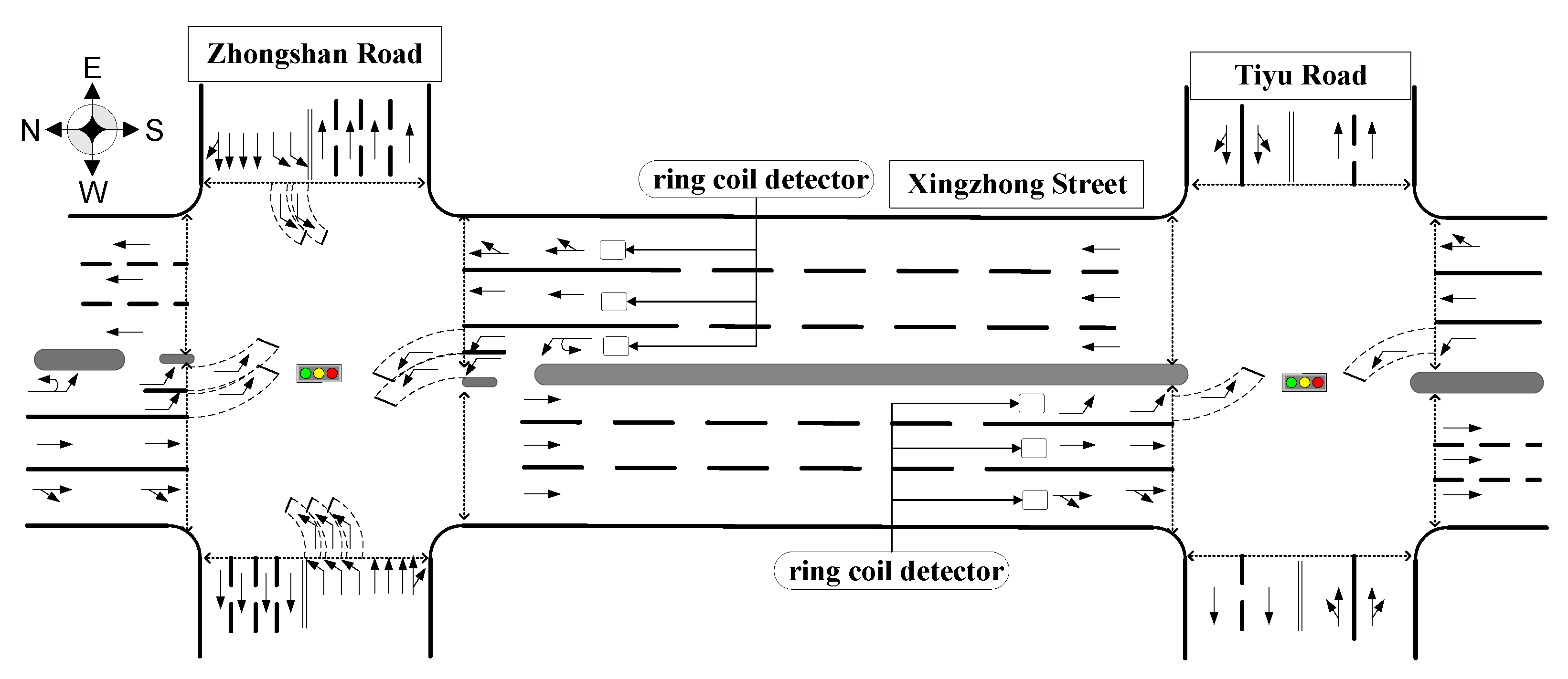
In this study, there are four traditional measurement of effectiveness (MOE) indices to evaluate the developed prediction method, such as mean absolute error (MAE), Mean absolute percentage error (MAPE), mean square error (MSE) and coefficient of variation (CV). CV is widely used in fields of engineering or applied statistics when doing quality assurance studies. The detailed calculation formulas of these indices are expressed as follows:

$$MAE=\frac{1}{N}{\displaystyle \sum }_{n=1}^N\left|v_{\left(d,t\right)}-{\widehat{v}}_{\left(d,t\right)}\right|$$

(2)

$$MAPE=\frac{1}{N}{\displaystyle \sum }_{n=1}^N\frac{\left|v_{\left(d,t\right)}-{\widehat{v}}_{\left(d,t\right)}\right|}{v_{\left(d,t\right)}}$$

(3)

$$MSE=\frac{1}{N}{\displaystyle \sum }_{n=1}^N{\left(v_{\left(d,t\right)}-{\widehat{v}}_{\left(d,t\right)}\right)}^2$$

(4)

$$CV=\frac{\widehat{\sigma }}{\widehat{\mu }}$$

(5)

where $v_{\left(d,t\right)}$ and ${\widehat{v}}_{\left(d,t\right)}$ represent the actual and the predicted traffic speeds, respectively. $N$ is the number of test samples, $\widehat{\mu }$ denotes the average value of predicted speed, and $\widehat{\sigma }$ is the standard deviation of the predicted speed.

In this study, the stacking regression models contain three basic underlying learners of SVM, CATBOOST, and KNN, and the meta-regressor is the ridge regression method. The framework of the proposed method is showed in Figure 2.

4. Case Study

The proposed model will be evaluated with traffic data collected by ITS with Internet Plus from the department of the Zhongshan Traffic Police Detachment. Zhongshan is one of the pilot cities to implement ITS applications in China, which has the ability to automatically collect city-level traffic flow data at signalized intersections. The testbed is selected on Xingzhong Rd with two-way six motorized lanes, which is the busiest and most congested south–north corridors in the Zhongshan downtown area [39]. Northbound and southbound traffic flow were collected by loop detectors located several meters before the stopline at the signalized intersection between Zhongshan Rd. and Tiyu Rd., and the two-way link travel speed was collected by floating car detection in Figure 3. In this study, the pilot dataset with the time interval of 1 h on Xingzhong Rd, was recorded over five weeks from 21 October to 24 November 2018. Referring to the correlation analysis mentioned above, this paper selected 10 representative features to calculate the Pearson correlation analysis as shown in

Table 2. Pearson correlation coefficients for northbound traffic on Xingzhong Rd.

	v(d,t)	v(d−1,t)	v(d−2,t)	v(d−3,t)	v(d−1,t+1)	v(d−2,t+1)	v(d−3,t+1)	flow(d,t)	v1(d,t)	v2(d,t)
v(d,t)	1	0.835	0.813	0.808	0.687	0.684	0.675	−0.801	0.782	0.874
v(d−1,t)	0.835	1	0.835	0.811	0.732	0.685	0.687	−0.796	0.775	0.823
v(d−2,t)	0.813	0.835	1	0.835	0.695	0.736	0.685	−0.793	0.751	0.796
v(d−3,t)	0.808	0.811	0.835	1	0.690	0.695	0.734	−0.797	0.734	0.803
v(d−1,t+1)	0.687	0.732	0.695	0.690	1	0.835	0.811	−0.750	0.689	0.692
v(d−2,t+1)	0.684	0.685	0.736	0.695	0.835	1	0.835	−0.739	0.668	0.671
v(d−3,t+1)	0.675	0.687	0.685	0.734	0.811	0.835	1	−0.737	0.644	0.680
flow(d,t)	−0.801	−0.796	−0.793	−0.797	−0.750	−0.739	−0.737	1	−0.772	−0.829
v1(d,t)	0.782	0.775	0.751	0.734	0.689	0.668	0.644	−0.772	1	0.815
v2(d,t)	0.874	0.823	0.796	0.803	0.692	0.671	0.680	−0.829	0.815	1

and

Table 3. Pearson correlation coefficients for southbound traffic on Xingzhong Rd.

	v(d,t)	v(d−1,t)	v(d−2,t)	v(d−3,t)	v(d−1,t+1)	v(d−2,t+1)	v(d−3,t+1)	flow(d,t)	v1(d,t)	v2(d,t)
v(d,t)	1	0.752	0.716	0.706	0.540	0.518	0.536	−0.694	0.834	0.870
v(d−1,t)	0.752	1	0.778	0.735	0.614	0.562	0.543	−0.716	0.757	0.789
v(d−2,t)	0.716	0.778	1	0.773	0.557	0.614	0.563	−0.712	0.700	0.766
v(d−3,t)	0.706	0.735	0.773	1	0.543	0.554	0.616	−0.697	0.687	0.784
v(d−1,t+1)	0.540	0.614	0.557	0.543	1	0.778	0.735	−0.639	0.528	0.603
v(d−2,t+1)	0.518	0.562	0.614	0.554	0.778	1	0.773	−0.627	0.515	0.592
v(d−3,t+1)	0.536	0.543	0.563	0.616	0.735	0.773	1	−0.623	0.508	0.604
flow(d,t)	−0.694	−0.716	−0.712	−0.697	−0.639	−0.627	−0.623	1	−0.699	−0.773
v1(d,t)	0.834	0.757	0.700	0.687	0.528	0.515	0.508	−0.699	1	0.809
v2(d,t)	0.870	0.789	0.766	0.784	0.603	0.592	0.604	−0.773	0.809	1

.

Where, v_1(d,t)(v_2(d,t)) represents the tth-hour upstream(downstream) speed on the dth day.

Table 2 and Table 3 show the correlation between different spatial-temporal speed and flow, respectively. One can find that the correlation between current interval and the same historical interval in the past days is relatively high, regardless of the day of week. The link travel speed at time t also has a strong correlation with the upstream and downstream ones at the lowest of over 0.782. However, the correlation between the speed at interval t and t + 1 in the historical days decreases with the passage of time. This is because the traffic flow has a certain randomness and the current traffic state at interval t has a significant difference from the interval t + 1 in the historical days. In addition, the current speed has a negative correlation with the current flow, which indicates that the higher the speed is, the lower the flow is. Notably, the correlation between the variables on the northbound links is higher than the southbound, which is mainly because the northbound traffic is relatively more stable and has less fluctuation than the southbound. According to statistical analysis, those variables that have a high correlation degree of ≥0.6 [40] could be allowed for detrending. After detrending, the residual set would be inputs in this study. Input variables of the proposed DDESLM model are shown in

Table 4. Input candidates of the proposed prediction model in this study.

Representative Feature	Descriptions
${\widehat{v}}_{\left(d,t+h\right)}^{dif}$	Predicted speed difference between predicted speed and daily average value at time t + h belonging to the dth day
h	Prediction time step into the future, h ≥ 1
$v_{\left(d,t\right)}^{dif}$	Speed difference between measured speed and daily average value at time t belonging to the dth day
$v_{\left(d-1,t\right)}^{dif}$	Speed difference between measured speed and daily average value at time t belonging to the d-1th day
$v_{\left(d-2,t\right)}^{dif}$	Speed difference between measured speed and daily average value at time t belonging to the d-2th day
$v_{\left(d-3\right)}^{dif}$	Speed difference between measured speed and daily average value at time t belonging to the d-3th day
$flo{w}_{\left(d,t\right)}^{dif}$	Flow difference between measured traffic flow and daily average value at time t belonging to the dth day
$v_{\left(d,t\right)}^{updif}$	Upstream speed difference between measured speed and daily average value at time t belonging to the dth day
$v_{\left(d,t\right)}^{downdif}$	Downstream speed difference between measured speed and daily average value at time t belonging to the dth day

.

5. Discussion

The experimental in this study is operated on a Windows 10 64-bit PC with 4.00 GHz Intel(R) Core(TM) i7-4790K CPU and a 16 GB memory. The software used in our experiment is Jupyter 6.1.1 and Python 3.6. The key parameters of four benchmark models are shown in

Table 5. The key parameters of four benchmark models in Python.

Model	Base Learner	Mega Learner	Descriptions
KNN	√		n_neighbors = 3
CATBOOST	√		Depth = 8, learning_rate = 0.8, loss_function = ‘RMSE’, random_seed = 18
SVM	√		C = 100, gamma = 0.01, kernel = ‘rbf’
RIDGE REGRESSION		√	Alpha = 17, random_state = 1

.

Where n_neighbors mean the number of nearest neighbors; depth denotes the depth of trees; learning_rate is used for reducing the gradient step, which affects the overall time of training: The smaller the value, the more iterations are required for training; loss_function represents the a certain metric during model training; C limits the importance of each point; gamma controls the width of the Gaussian kernel; kernel means kernel function; alpha means regularization strength; and random_state means the seed of the pseudo random number generator to use when shuffling the data while random_seed is the same with random_state.

The proposed forecasting models in this study are evaluated by comparing with four other predictors: SVM, CATBOOST, KNN, and BAGGING (the average result of SVM, CATBOOST, and KNN into an ensemble learning). SVM could deal with overfitting problem and have good generalization performance because SVM can construct a mapping from one dimensional input vector into high-dimensional space by the use of reproducing kernels. Furthermore, the SVM is also slow in the test phase due to the high algorithm complexity and needs a large memory capacity to calculate. CATBOOST uses an efficient gradient modification of ordered boosting to overcome the problem of target leakage, and it performs well in small datasets, but training a CATBOOST model requires a great deal of time and compute memory. KNN is suitable for small datasets but it is usually hysteretic in time series. BAGGING is a combination of KNN, SVM, and CATBOOST, and outperforms each individual method.

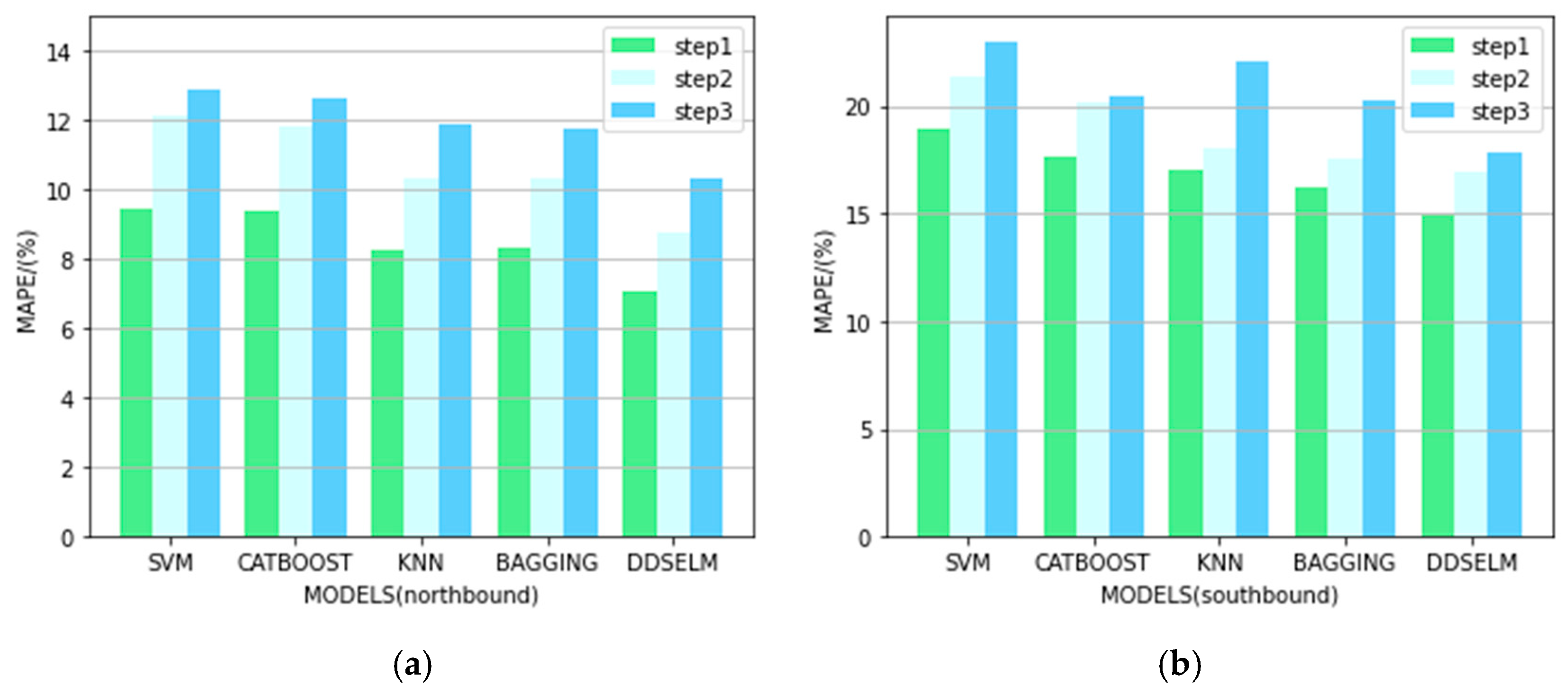
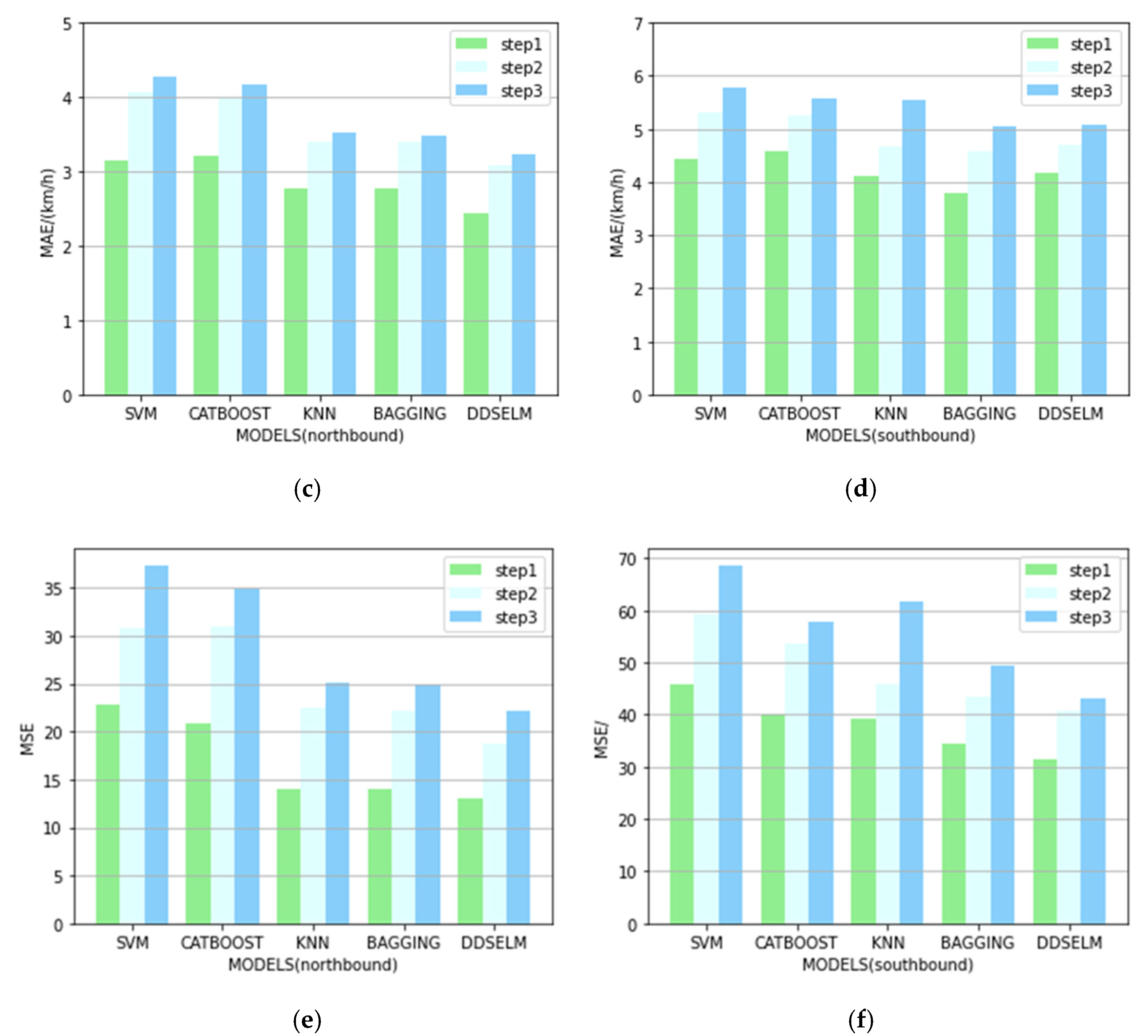
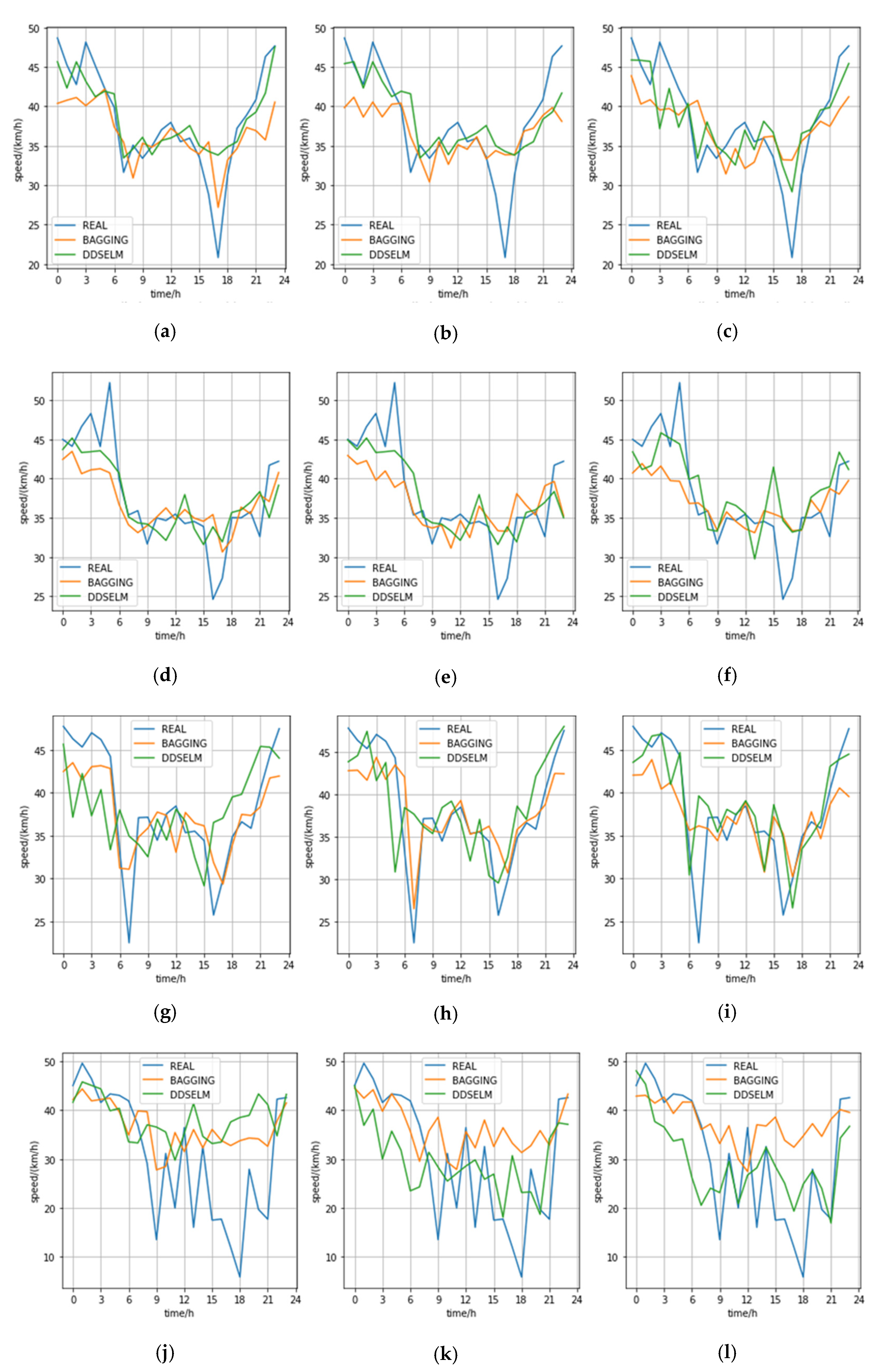
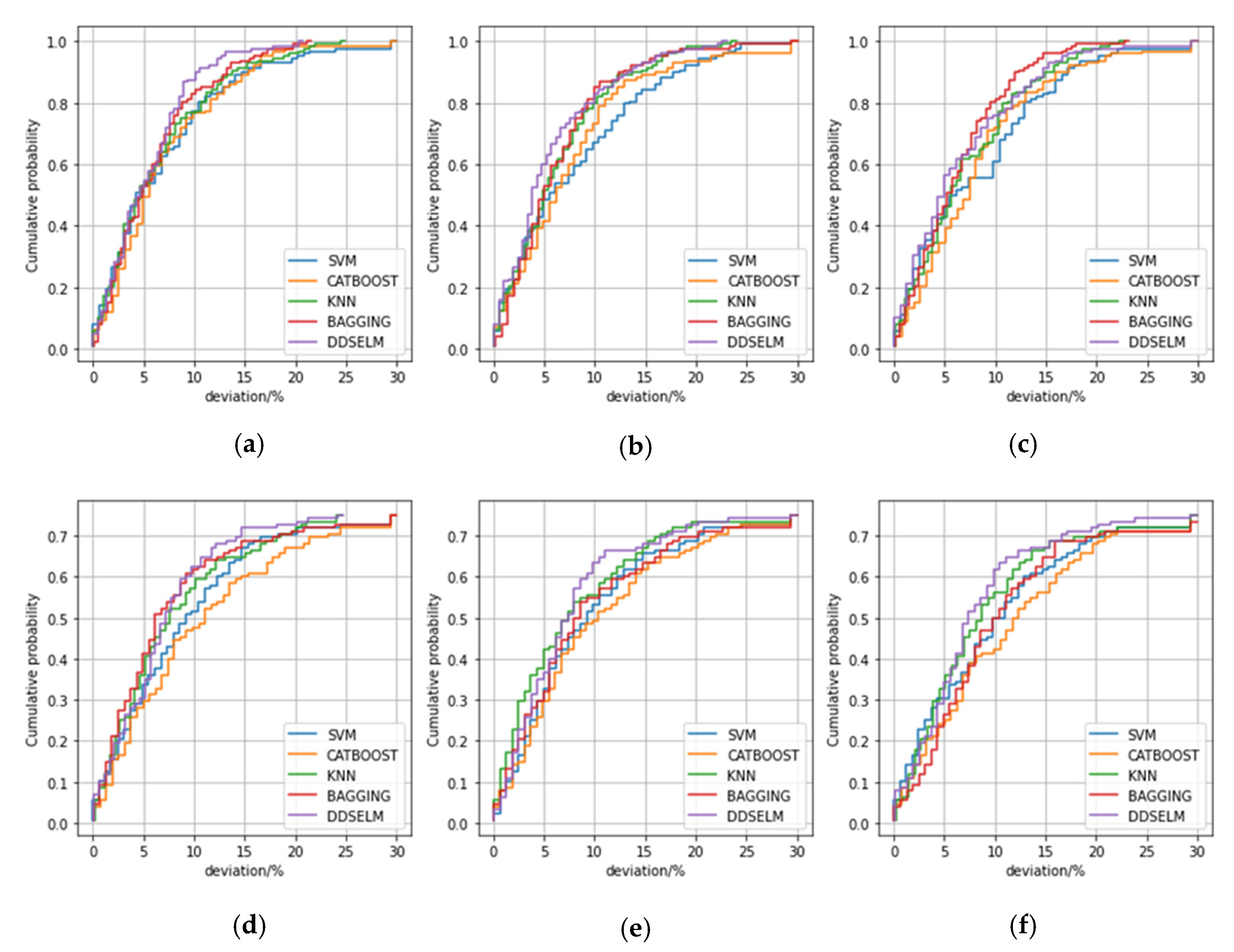
5.1. Prediction Accuracy

The MOE results of the proposed DDSELM and other four benchmark models are drawn in Figure 4 on southbound and northbound road links. Each subfigure shows one performance index of five prediction models under three scenarios with three kinds of prediction steps [1 h (60 min), 2 h (120 min), 3 h (180 min)] into the future. For the different steps in Figure 4, one can find that the prediction accuracy of each models is decreasing with the increase of the prediction step regardless of the southbound or northbound links. This result is consistent with the results of existing studies [30,33], which found that it is particularly difficult to conduct multi-step-ahead prediction due to the randomness and uncertainty of the travel speed.

As shown in Figure 4, the ensemble learning models of the proposed DDSELM can yield many more benefits than individual models (SVM, CATBOOST, and KNN) and ensemble one (BAGGING) regardless of the ahead-prediction step. In particular, the developed DDSELM in this study can outperform four kinds of benchmark models. In particular, the KNN, an individual method, performs better than SVM and CATBOOST for one-step-ahead prediction, but it also suffers many more errors than the two other individual ones for three-step-ahead prediction in Figure 4a. Compared with KNN, DDSELM always has good performance regardless of the road direction and prediction steps, among which the MAPE of northbound DDSELM is 1.16% lower (7.08% versus 8.24%) than KNN in one-step-ahead prediction, 1.58% (8.77% versus 10.35%) in two-step-ahead prediction, and 1.56% (10.34% versus 11.90%) in three-step-ahead prediction, respectively. In Figure 4b, the MAPE of southbound DDSELM is 2.10% lower (14.90% versus 17.00%) than KNN in one-step-ahead prediction, 1.05% (16.99% versus 18.04%) in two-step-ahead prediction, and 4.30% (17.82% versus 22.12%) in three-step-ahead prediction, respectively. Notably, the prediction accuracy of the northbound DDSELM is better than southbound, which might be that the correlation between travel speed of the northbound links is higher than the southbound.

Furthermore, a more detailed analysis about the two ensemble models of DDSELM and BAGGING was conducted for the multi-step-ahead prediction over a weekday of Wednesday and a weekend of Saturday in Figure 5. Regardless of the ahead-prediction step size, the performance of these two ensemble models performs much better during the off-peak hours (9:00~16:00) than peak ones (7:00~8:00 and 17:00~18:00), and DDSELM is especially better than BAGGING. The reason might be because BAGGING only uses the average of all underlying prediction outputs to make up for the shortcomings of each individual prediction model, but DDSELM uses the ridge regression algorithm in the mega learner. The ridge regression uses L2 regularization for reducing the prediction error. During the peak hours, both southbound and northbound predictions have much higher accuracy in the morning peak period (7:00~9:00) than evening (17:00~19:00). As far as the evening peak period, single-step prediction is better than multi-step-ahead for the northbound segments. This is because the traffic flow during the evening peak hours was much larger than the morning and there was a sharp drop in travel speed around 17:00. Therefore, there is a certain difference in the accuracy of two-way prediction. Compared with the accuracy of weekdays, accuracy of one-step-ahead northbound prediction on weekends slightly increases (8.36% to 7.54%), while the accuracy of one-step-ahead southbound prediction decreases (9.60% to 13.79%). The multi-step prediction (two-step-ahead prediction and three-step prediction) also has a similar trend, namely, prediction accuracy increases in northbound while decreasing in the southbound direction. This may be because the southbound data itself is less relevant than the northbound data in Table 2 and Table 3.

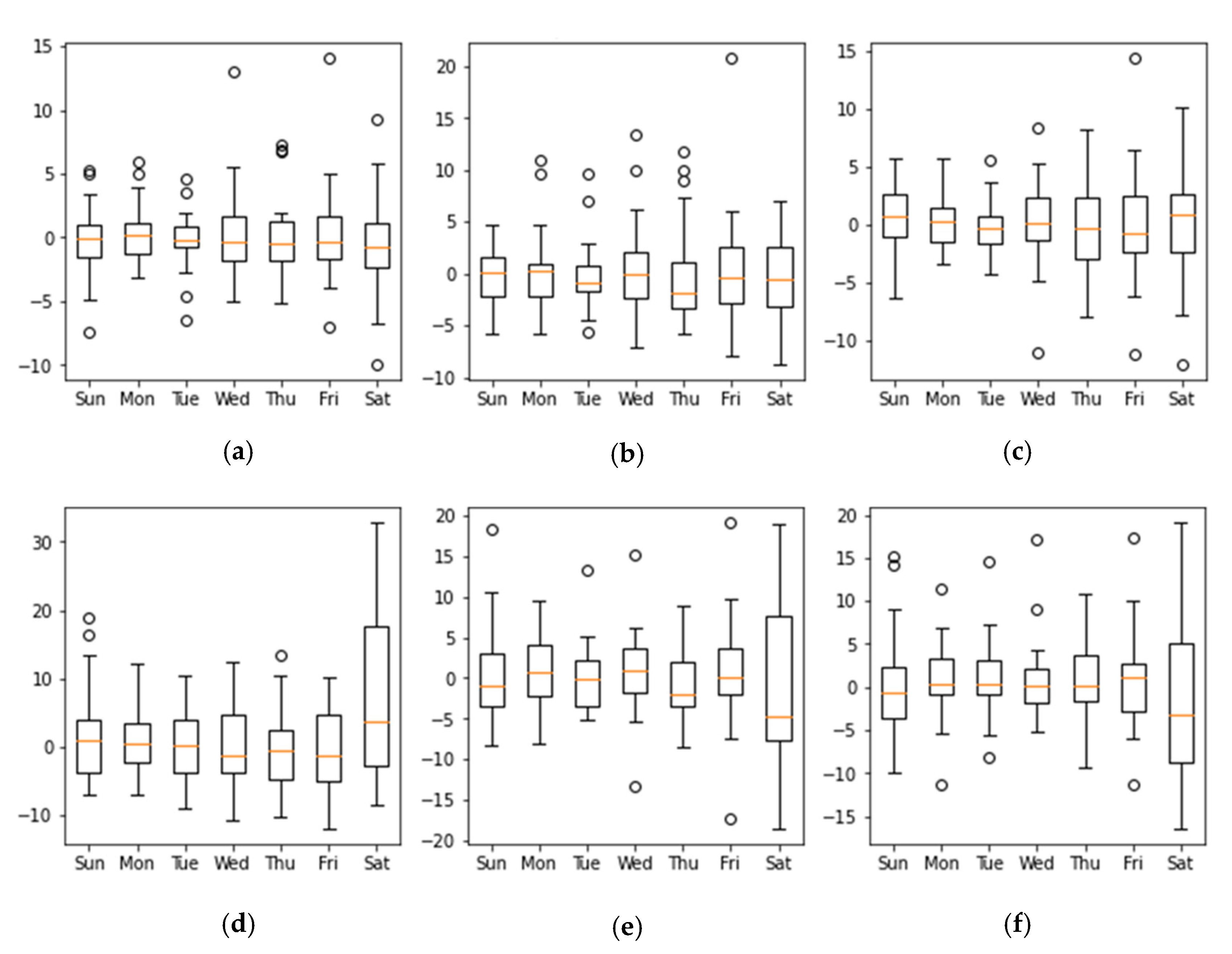
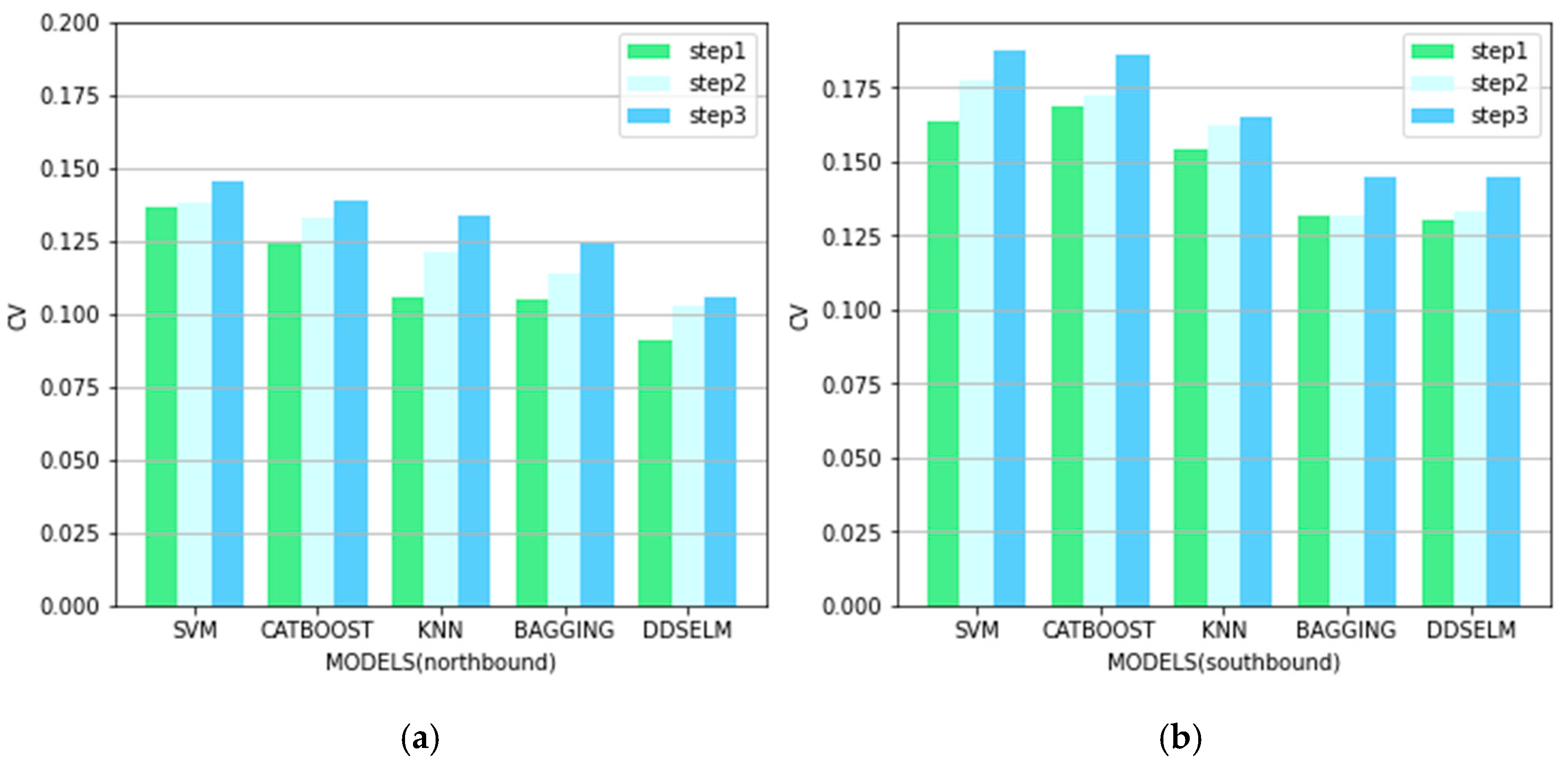
5.2. Prediction Stability

Figure 6 shows the boxplots for the one-week prediction error and one will find that, for the northbound prediction, the number of positive errors is larger than the number of negative errors for different prediction steps; that is, most northbound prediction outputs are larger than the observed values, whereas the number of positive errors is roughly equal to the number of negative errors for the southbound traffic. For the same prediction step, the fluctuation of the northbound prediction errors is smaller than southbound. For example, the northbound one-step prediction error range is [−7.57,17.12], while southbound is [−16.06,17.50].

The cumulative distribution function (CDF) is an integral of the probability density function, which provides a complete description of the probability distribution of a real random variable. The CDFs of five prediction models are plotted in Figure 7, where the x axis is the deviation of prediction error, and the y axis is the cumulative probability. One can found out that the sequence of model prediction performance from good to bad is DDSELM, BAGGING, KNN, CATBOOST, and SVM. The DDSELM also can provide much more stability than others. For northbound prediction, the 83.33% of its one-step-ahead prediction has error less than 10%, 71.42% for two-step-ahead, and 70.83% for three-step-ahead, respectively. Correspondingly, the prediction error of less than 10% accounts for 71.42% for one-step-ahead, 60.11% for two-step-ahead, and 58.76% for three-step-ahead for southbound prediction, respectively.

The CV is an important indicator to measure the diversity of data. Compared with other prediction models, the CV of DDSELM has the minimum score regardless of prediction step as shown in Figure 8. Compared with other four models, DDSELM has lower CV, reaching 0.09, 0.10, and 0.11 for one-step-ahead, two-step-ahead, and three-step-ahead prediction, respectively, in Figure 8a. In the south direction, the CVs are similar to those of north direction except the south direction has higher CVs because of the lower correlation mentioned in Section 4.

6. Conclusions

In order to tackle the challenge of multi-step traffic speed prediction, we proposed an ensemble model, i.e., the Detrending and Direct Strategy Ensemble Learning Model (DDSELM). The detrending technique could separate original dataset into mean trends and residuals, and the direct strategy could decrease the cumulative error in the prediction process. To validate the effectiveness of our model, we used several benchmark models as a comparison model, including SVM, CATBOOST, KNN, and BAGGING, based on a field dataset collected in the city of Zhongshan, China. Predictive results showed that our model outperformed four benchmark ones in terms of the MAPE, MAE, MSE, and CV under three prediction intervals. For one-step-ahead prediction, the MAPE of DDSELM for northbound segments is 7.08% (14.90% for southbound segments). For two-step-ahead and three-step-ahead prediction, the MAPE of DDSELM for northbound segments is 8.77% and 10.34% (16.99% and 17.82% for southbound segments), respectively. In future works, it is necessary to consider the impact of road network characteristics and specific incidents on prediction accuracy. Moreover, the proposed model can also be integrated into some advanced ITS to alleviate traffic congestion, for example, real-time route planning systems, traffic management systems, and traffic signal control systems.

References

1. Sun, S.; Huang, R.; Gao, Y. Network-scale traffic modeling and forecasting with graphical lasso and neural networks. J. Transp. Eng. 2012, 11, 1358–1367. [Google Scholar] [CrossRef] [Green Version]
2. Schrank, D.; Eisele, B.; Lomax, T. 2019 Urban Mobility Scorecard; Texas A&M Transportation Institute: College Station, TX, USA, 2019. [Google Scholar]
3. Qureshi, K.N.; Abdul, H.A. A survey on intelligent transportation systems. Middle-East J. Sci. Res. 2013, 15, 629–642. [Google Scholar]
4. Lin, Y.; Wang, P.; Ma, M. Intelligent transportation system (ITS): Concept, challenge and opportunity. In Proceedings of the IEEE 3rd International Conference on Big Data Security on Cloud (Big Data Security), IEEE International Conference on High Performance and Smart Computing (hpsc), and IEEE International Conference on Intelligent Data and Security (ids), Beijing, China, 26–28 May 2017. [Google Scholar]
5. Tang, J.; Liu, F.; Zou, Y.; Zhang, W.; Wang, Y. An improved fuzzy neural network for traffic speed prediction considering periodic characteristic. IEEE Trans. Intell. Transp. Syst. 2017, 18, 2340–2350. [Google Scholar] [CrossRef]
6. Vlahogianni, E.; Matthew, G.; Golias, J. Short-term traffic forecasting: Where we are and where we’re going. Transp. Res. Part C Emerg. Technol. 2014, 43, 3–19. [Google Scholar] [CrossRef]
7. Zhang, Z.; Li, M.; Lin, X.; Wang, Y.; He, F. Multistep speed prediction on traffic networks: A deep learning approach considering spatio-temporal dependencies. Transp. Res. Part C Emerg. Technol. 2019, 105, 297–322. [Google Scholar] [CrossRef]
8. Alajali, W.; Zhou, W.; Wen, S.; Wang, Y. Intersection Traffic Prediction Using Decision Tree Models. Symmetry 2018, 10, 386. [Google Scholar] [CrossRef] [Green Version]
9. Chang, H.; Lee, Y.; Yoon, B.; Baek, S. Dynamic near-term traffic flow prediction: System-oriented approach based on past experiences. IET Intell. Transp. Syst. 2012, 6, 292–305. [Google Scholar] [CrossRef]
10. Ahmed, M.; Cook, A. Analysis of freeway traffic time-series data by using Box-Jenkins techniques. Transp. Res. Rec. 1979, 722, 1–9. [Google Scholar]
11. Voort, M.; Dougherty, M.; Watson, S. Combining Kohonen maps with ARIMA time series models to forecast traffic flow. Transp. Res. Part C Emerg. Technol. 1996, 4, 307–318. [Google Scholar] [CrossRef] [Green Version]
12. Williams, B.; Hoel, L. Modeling and forecasting vehicular traffic flow as a seasonal ARIMA process: Theoretical basis and empirical results. J. Transp. Eng. 2003, 129, 664–672. [Google Scholar] [CrossRef] [Green Version]
13. Kumar, S.; Lelitha, V. Short-term traffic flow prediction using seasonal ARIMA model with limited input data. Eur. Transp. Res. Rev. 2015, 7, 21. [Google Scholar] [CrossRef] [Green Version]
14. Okutani, I.; Stephanedes, Y. Dynamic prediction of traffic volume through Kalman filtering theory. Transp. Res. Part Meth. 1984, 18, 1–11. [Google Scholar] [CrossRef]
15. Guo, J.; Huang, W.; Williams, B. Adaptive Kalman filter approach for stochastic short-term traffic flow rate prediction and uncertainty quantification. Transp. Res. Part C Emerg. Technol. 2014, 43, 50–64. [Google Scholar] [CrossRef]
16. Mir, Z.; Filali, F. An adaptive Kalman filter based traffic prediction algorithm for urban road network. In Proceedings of the IEEE 12th International Conference on Innovations in Information Technology (IIT), Al-Ain, United Arab Emirates, 28–30 November 2016. [Google Scholar]
17. Zambrano-Martinez, J.; Calafate, C.; Soler, D.; Lemus-Zúñiga, L.; Cano, J.; Manzoni, P.; Gayraud, T. A centralized route-management solution for autonomous vehicles in urban areas. Electronics 2019, 8, 722. [Google Scholar] [CrossRef] [Green Version]
18. Vlahogianni, E.; Golias, J.; Matthew, G. Short-term traffic forecasting: Overview of objectives and methods. Transp. Rev. 2004, 24, 533–557. [Google Scholar] [CrossRef]
19. Dougherty, M. A review of neural networks applied to transport. Transp. Res. Part C Emerg. Technol. 1995, 3, 247–260. [Google Scholar] [CrossRef]
20. Vlahogianni, E.; Matthew, G.; Golias, J. Optimized and meta-optimized neural networks for short-term traffic flow prediction: A genetic approach. Transp. Res. Part C Emerg. Technol. 2005, 13, 211–234. [Google Scholar]
21. Zhang, N.; Guan, X.; Cao, J.; Wang, X.; Wu, H. Wavelet-HST: A Wavelet-Based Higher-Order Spatio-Temporal Framework for Urban Traffic Speed Prediction. IEEE Access 2019, 7, 118446–118458. [Google Scholar] [CrossRef]
22. Cai, P.; Wang, Y.; Lu, G.; Chen, P.; Ding, C.; Sun, J. A spatiotemporal correlative k-nearest neighbor model for short-term traffic multistep forecasting. Transp. Res. Part C Emerg. Technol. 2016, 62, 21–34. [Google Scholar] [CrossRef]
23. Ma, X.; Tao, Z.; Wang, Y.; Yu, H.; Wang, Y. Long short-term memory neural network for traffic speed prediction using remote microwave sensor data. Transp. Res. Part C Emerg. Technol. 2015, 54, 187–197. [Google Scholar] [CrossRef]
24. Yao, B.; Chen, C.; Cao, Q.; Jin, L.; Zhang, M. Short-term traffic speed prediction for an urban corridor. Comput. Aided Civ. Inf. 2017, 32, 154–169. [Google Scholar] [CrossRef]
25. Dong, X.; Lei, T.; Jin, S.; Hou, Z. Short-Term Traffic Flow Prediction Based on XGBoost. In Proceedings of the IEEE 7th Data Driven Control and Learning Systems Conference (DDCLS), Enshi, China, 25–27 May 2018. [Google Scholar]
26. Yao, X.; Liu, Y. Ensemble structure of evolutionary artificial neural networks. In Proceedings of the IEEE International Conference on Evolutionary Computation, Nagoya, Japan, 20–22 May 1996. [Google Scholar]
27. Vennelakanti, A.; Shreya, S.; Rajendran, R.; Sarkar, D.; Muddegowda, D.; Hanagal, P. Traffic sign detection and recognition using a cnn ensemble. In Proceedings of the IEEE International Conference on Consumer Electronics (ICCE), Las Vegas, NV, USA, 11–13 January 2019. [Google Scholar]
28. Lukáš, R. Traffic speed prediction using ensemble kalman filter and differential evolution. In Proceedings of the 6th International Conference on Traffic and Logistic Engineering (ICTLE 2018), Bangkok, Thailand, 3–5 August 2018. [Google Scholar]
29. Xiao, J.; Xiao, Z.; Wang, D.; Bai, J.; Havyarimana, V.; Zeng, F. Short-term traffic volume prediction by ensemble learning in concept drifting environments. Knowl.-Based Syst. 2019, 164, 213–225. [Google Scholar] [CrossRef]
30. Xiao, J. SVM and KNN ensemble learning for traffic incident detection. Phys. A Stat. Mech. Appl. 2019, 517, 29–35. [Google Scholar] [CrossRef]
31. Zhang, S.; Zhou, L.; Chen, X.; Zhang, L.; Li, L.; Li, M. Network-wide traffic speed forecasting: 3D convolutional neural network with ensemble empirical mode decomposition. Comput. Aided Civ. Inf. 2020, 35, 1132–1147. [Google Scholar] [CrossRef]
32. Papathanasopoulou, V.; Markou, I.; Antoniou, C. Online calibration for microscopic traffic simulation and dynamic multi-step prediction of traffic speed. Transp. Res. Part C Emerg. Technol. 2016, 68, 144–159. [Google Scholar] [CrossRef]
33. Cox, D. Prediction by exponentially weighted moving averages and related methods. J. R. Stat. Soc. Ser. B (Methodol.) 1961, 23, 414–422. [Google Scholar] [CrossRef]
34. Zhan, X.; Zhang, S.; Szeto, W.; Chen, X. Multi-step-ahead traffic speed forecasting using multi-output gradient boosting regression tree. J. Intell. Transp. Syst. 2020, 24, 125–141. [Google Scholar] [CrossRef]
35. Pearson, K. Mathematical contributions to the theory of evolution (III): Regression, heredity, and panmixia. Philos. Trans. R. Soc. Lond. Ser. A 1895, 187, 253–318. [Google Scholar]
36. Li, Z.; Li, Y.; Li, L. A comparison of detrending models and multi-regime models for traffic flow prediction. IEEE Intell. Transp. Syst. Mag. 2014, 6, 34–44. [Google Scholar]
37. Ren, Y.; Zhang, L.; Suganthan, P. Ensemble classification and regression-recent developments, applications and future directions. IEEE Comput. Intell. Mag. 2016, 11, 41–53. [Google Scholar] [CrossRef]
38. Wolpert, D. Stacked generalization. Neu. Netw. 1992, 5, 241–259. [Google Scholar] [CrossRef]
39. Feng, B.; Xu, J.; Lin, Y.; Li, P. A period-specific combined traffic flow prediction based on travel speed clustering. IEEE Access 2020, 8, 85880–85889. [Google Scholar] [CrossRef]
40. Zheng, L.; Yang, J.; Chen, L.; Sun, D.; Liu, W. Dynamic spatial-temporal feature optimization with ERI big data for Short-term traffic flow prediction. Neurocomputing 2020, 412, 339–350. [Google Scholar] [CrossRef]
Figure 1. The framework of direction strategy
Applsci 11 04423 g001
Figure 2. The framework of the proposed predictor (DDSELM) in this study.
Applsci 11 04423 g002
Figure 3. The layout of pilot intersections in the city of Zhongshan, China.
Applsci 11 04423 g003
Figure 4. MOEs of five prediction models:(a) MAPE of five models in northbound; (b) MAPE of five models in southbound; (c) MAE of five models in northbound; (d) MAE of five models in southbound; (e) MSE of five models in northbound; (f) MSE of five models in southbound.
Applsci 11 04423 g004aApplsci 11 04423 g004b
Figure 5. The prediction comparisons by two ensemble methods on Wednesday and Saturday:(a) one-step-ahead prediction result on Wednesday in northbound; (b) two-step-ahead prediction result on Wednesday in northbound; (c) three-step-ahead prediction result on Wednesday in northbound; (d) one-step-ahead prediction result on Saturday in northbound; (e) two-step-ahead prediction result on Saturday in northbound; (f) three-step-ahead prediction result on Saturday in northbound; (g) one-step-ahead prediction result on Wednesday in southbound; (h) two-step-ahead prediction result on Wednesday in southbound; (i) three-step-ahead prediction result on Wednesday in southbound; (j) one-step-ahead prediction result on Saturday in southbound; (k) two-step-ahead prediction result on Saturday in southbound; (l) three-step-ahead prediction result on Saturday in southbound.
Applsci 11 04423 g005
Figure 6. Comparison between the real speed and the predicted speed in boxplots: (a) one-step-ahead prediction error in northbound; (b) two-step-ahead prediction error in northbound; (c) three-step-ahead prediction error in northbound; (d) one-step-ahead prediction error in southbound; (e) two-step-ahead prediction error in southbound; (f) three-step-ahead prediction error in southbound.
Applsci 11 04423 g006
Figure 7. Cumulative distribution function of five prediction models: (a) one-step-ahead prediction CDF in northbound; (b) two-step-ahead prediction CDF in northbound; (c) three-step-ahead prediction CDF in northbound; (d) one-step-ahead prediction error in southbound; (e) two-step-ahead prediction CDF in southbound; (f) three-step-ahead prediction CDF in southbound.
Applsci 11 04423 g007
Figure 8. Performance of five predictive models’ results in CVs: (a) CVs of predictive results in northbound; (b) CVs of predictive results in southbound
Applsci 11 04423 g008