Direct Calculation of the Group Velocity for Two-Dimensional Complex, Composite and Periodic Structures Using a Wave and Finite Element Scheme

Abstract

Guided waves have immense potential for structural health monitoring applications in numerous industries including aerospace. It is necessary to evaluate guided wave dispersion characteristics, i.e., group velocity and phase velocity profiles, for using them effectively. For complex structures, the profiles can have highly irregular shapes. In this work, a direct method for calculating the group velocity profiles for complex, composite, and periodic structures using a wave and finite element scheme is presented. The group velocity calculation technique is easy to implement, highly computationally efficient, and works with the standard finite element formulation. The major contribution is summarised in the form of a comprehensive algorithm for calculating the group velocity profiles. The method is compared with the existing analytical and numerical methods for calculation of dispersion curves. Finally, an experimental study in a multilayered composite plate is conducted and the results are found to be in good agreement. The technique is suitable to be used in all guided wave application areas such as material characterisation, non-destructive testing, and structural health monitoring.

1. Introduction

Structural health monitoring (SHM) in the aerospace sector has the potential to reduce costs and increase reliability [1]. A number of nondestructive inspection techniques are already applied in the aerospace industry such as radiography [2], acoustic emission [3], eddy current [4], and ultrasonic inspection [5]. The use of advanced composite structures has also introduced an added layer of complexity where the failure modes are complex [6] and damage may occur between layers. Guided waves present a suitable SHM technique for thin structures [7,8,9]. They can travel large distances and interact with defects. Hence, they can be used for detection, localisation, and identification of damage [10,11].

Ultrasonic guided waves are guided by the traction free top and bottom surfaces of thin plate-like structures. They are generated due to the constructive and destructive interference and superposition of pressure waves and shear vertical waves undergoing multiple reflections from the boundaries [12]. Guided waves in plates can be classified into three broad categories based on their polarisation [13]: (a) symmetric (S) waves polarised perpendicular to the plane of the plate with the plate surfaces displacing out of phase, (b) anti-symmetric (A) waves polarised perpendicular to the plane of the plate with the plate surfaces displacing in phase, and (c) shear horizontal (SH) waves polarised in the plane of the plate. SH waves can also be symmetric or anti-symmetric with respect to the mid-plane of the plate. In theory, an infinite number of guided wave modes can propagate in a plate. Hence, the conventional notation used to represent them is with a subscript n, where $\mathrm{n}=0,1,2,3\dots$, i.e., S_n and A_n. For SH_n, an even n denotes symmetric and an odd n denotes anti-symmetric waves. In multilayered structures, the elastic anisotropy results in quasi-Lamb waves and quasi-SH waves, which are mutually coupled, and the distinction is not as clear as in isotropic structures. It is still standard practice to adopt the nomenclature for guided waves in isotropic structures, which is followed here.

Guided wave dispersion curves provide important insight into the wave propagation in a structure. The group velocity curve shows the value of velocity versus the frequency. It is, however, important to calculate the change in the propagation direction of the group velocity versus the phase velocity for anisotropic materials. For isotropic plates with constant thickness, the group and phase velocities do not have angular dependence and the 2D profile is circular. This quickly becomes non-trivial in complex multilayered structures where the directions of wave propagation and energy propagation are different. The directional nature of composite structures creates another increase in complexity, where the 2D profile can take any shape depending on the composite layup. Nevertheless, identifying these characteristics is important for applications that use guided waves.

There are two main approaches for computing the dispersion properties: (a) analytical and (b) semi-analytical. The analytical methods consist of solving the governing differential equations by applying the appropriate boundary condition. They can further be divided into exact methods based on 3D elasticity theory and semi-exact methods based on approximate plate theories. The 3D elasticity method was used to calculate the phase velocity of composite lamina and laminate [14,15]. The exact methods are computationally intensive due to the transcendental equations used for multilayered composites. Therefore, approximate plate theories are employed to ensure the solutions are practical [16,17]. Recently, Biot’s general energy expression was applied to derive the group velocity vector of elastodynamic guided waves [18] in arbitrary layered structures. The semi-analytical methods use finite element (FE) approaches to model part of the structure and impose wave solutions in the propagation directions. The most well-known is the semi-analytical finite element (SAFE) method, where FE is used to model the cross-section, and a complex exponential function is used to describe the displacement field in the direction of wave propagation [19]. However, the SAFE method cannot be used to model truly periodic structures [20] that consist of identical substructures joined to form a continuous structure. The scaled boundary finite element method (SBFEM) was also applied in a similar semi-analytical framework for guided wave simulations [21] but only in isotropic structures. The wave and finite element (WFE) method has been developed over the last decade [22]. It combines FE and periodic structure theory to model wave propagation in periodic structures. It has been used in a number of research areas like structural identification [23], damage detection [24], multi-scale wave propagation [20], transient wave propagation [25], and wave steering in composites [26].

The main issue associated with the existing group velocity calculation methods is that they require custom formulations, which are difficult to implement, and none of them are able to handle truly periodic structures. Moreover, the group velocity from WFE was approximated by the slope of the wavenumber–frequency dispersion curve using finite differentiation. The principal novelty of the work exhibited in this manuscript is the calculation of the group velocity curves for two dimensional complex periodic and/or composite structures using a wave and finite element scheme without involving any finite differentiation. The approach is therefore free from computational errors, requirement for convergence checks, and additional computational cost implied by finite differentiation schemes. The use of periodic structures such as textile composites has become increasingly common in automotive and aerospace industries [27]. In order to employ guided-wave-based damage localization and identification, it is necessary to calculate the dispersion properties of such structures. The WFE scheme based calculation of dispersion curves has the following advantages:

• It is capable of handling both periodic and layered composite structures.
• It is relatively easier to implement and does not require custom FE formulation.
• It is computationally efficient and has minimal memory requirements.

The novelty of this work is the form of a comprehensive algorithm to calculate the dispersion properties of arbitrary plate-like structures. The paper is organised as follows: A brief introduction to the WFE method is presented in Section 2, followed by the energy and power flow considerations necessary for dispersion curve calculation. At the end of Section 2, the main algorithm is presented. The symbols used in this section are listed in

Table 1. List of symbols.

Symbol	Description
K, C, M	Stiffness, damping, and mass matrices
D	Dynamic stiffness matrix
$\mathit{\omega }$	Angular frequency
q	Vector of nodal degrees of freedom
f	Vector of internal forces
T	Transformation matrix
$\lambda$	Propagation constant
k	Wavenumber
$\mathfrak{T}$	Transfer matrix
$\mathit{\varphi }$	Modeshape vector
$E,P$	Energy and power
$c_g,c_p$	Group velocity and phase velocity
$\theta$	Propagation direction

. The method is compared with existing dispersion properties calculation techniques in Section 3, highlighting the main advantages of this approach. The comparison with experimental results is described in Section 4. This is followed by our conclusions in Section 6.

2. Dispersion Curve Calculation

The methodology for obtaining the dispersion curves of 2D periodic structures is presented in this section. The WFE method is used to obtain wave propagation characteristics, wavenumbers, and wave modes of the periodic waveguide. This is followed by the necessary energy and power flow considerations for calculating the group and phase velocities of guided wave modes. Finally, the algorithm for calculating the 2D group velocity profile is provided.

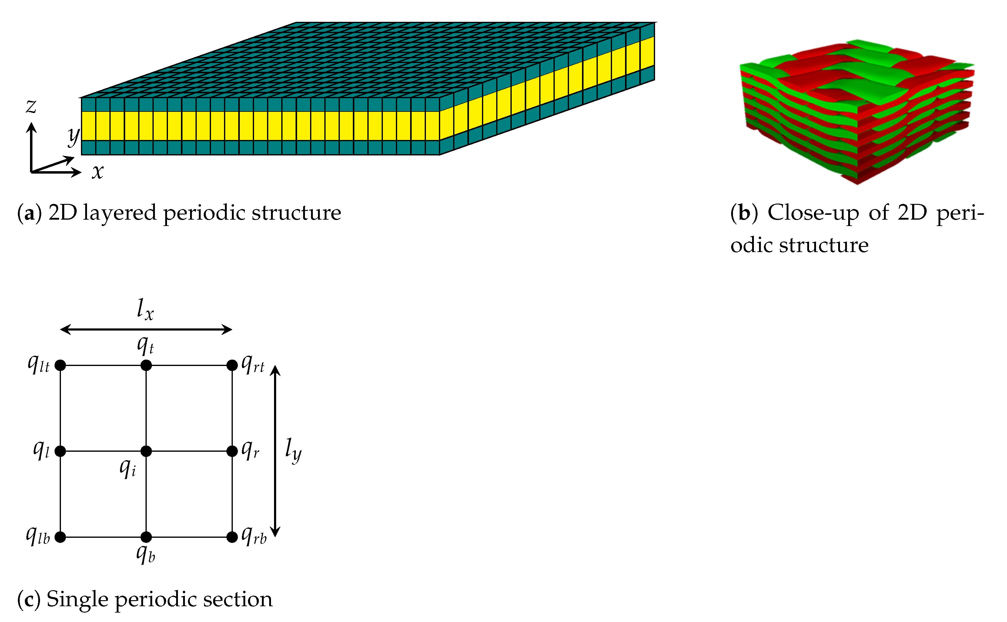
2.1. Wave and Finite Element Scheme

The WFE method has been developed over the last three decades and has been applied to a wide variety of structural calculations. The reader is referred to classical literature regarding this methodology [28,29,30] in order to obtain more information. With regard to two-dimensional periodic media as shown in Figure 1a, and a close-up example of such a structure shown in Figure 1b, the first step is to model a single periodic section using standard finite element software. There is no limitation with regard to the complexity of the cross-section to be modelled, making the method suitable for modelling layered media.

The finite element model of the periodic section is used to obtain the stiffness ($\mathbf{K}$), mass ($\mathbf{M}$), and damping ($\mathbf{C}$) matrices to set up the dynamic equilibrium as follows:

$$\left[\mathbf{K}+\mathrm{i}\omega \mathbf{C}-{\omega }^{\mathit{2}}\mathbf{M}\right]\mathbf{q}=\mathbf{f},$$

(1)

where $\mathbf{q}={\left\{{\mathbf{q}}_{lb}^{\mathrm{T}}{\mathbf{q}}_{rb}^{\mathrm{T}}{\mathbf{q}}_{lt}^{\mathrm{T}}{\mathbf{q}}_{rt}^{\mathrm{T}}{\mathbf{q}}_b^{\mathrm{T}}{\mathbf{q}}_r^{\mathrm{T}}{\mathbf{q}}_t^{\mathrm{T}}{\mathbf{q}}_l^{\mathrm{T}}{\mathbf{q}}_i^{\mathrm{T}}\right\}}^{\mathrm{T}}$ is the vector of nodal degrees of freedom. Each entry in this vector is formed by concatenating all nodes through the thickness, where ${(.)}^{\mathrm{T}}$ refers to a transpose. The size of each entry equals the number of nodal degrees of freedom times the number of concatenated nodes. The vector of internal forces $\mathbf{f}$ is ordered in the same way as $\mathbf{q}$. The coefficient matrix multiplying with $\mathbf{q}$ in Equation (1) is commonly known as the dynamic stiffness matrix $\mathbf{D}$. The dimension of Equation (1) can be reduced by applying the periodicity condition in the y-direction. For a free wave propagation scenario, where $k_y$ refers to the component of wavenumber in the y-direction, a transformation matrix $\mathbf{T}$ can be specified that reduces the nodal degrees of freedom vector as follows:

$$\mathbf{q}=\mathbf{T}{\mathbf{q}}_{\mathrm{red}},\mathrm{where}{\mathbf{q}}_{\mathrm{red}}={\left\{{\mathbf{q}}_{lb}^{\mathrm{T}}{\mathbf{q}}_{rb}^{\mathrm{T}}{\mathbf{q}}_b^{\mathrm{T}}\right\}}^{\mathrm{T}}.$$

(2)

The entries of matrix $\mathbf{T}$ are determined from the wave propagation constant ${\lambda }_y$, which, according to Bloch’s theorem, is given as ${\lambda }_y=e^{-\mathrm{i}{k}_y{l}_y}$, where $l_y$ is the height of the periodic section. The complete matrix depends on the ordering of the $\mathbf{q}$ vector; an example can be found in [28]. This projects all degrees of freedom on the nodes lying on the x-axis of the waveguide by imposing the periodic boundary conditions. A similar dimensional reduction is performed to obtain the reduced force vector ${\mathbf{f}}_{\mathrm{red}}$. Since there are no forces on the internal nodes, the internal nodal force vector ${\mathbf{f}}_b=0$. This helps in simplifying Equation (1) as follows [31]:

$$\left[\begin{array}{cc}{\mathbf{D}}_{ll}& {\mathbf{D}}_{lr}\\ {\mathbf{D}}_{rl}& {\mathbf{D}}_{rr}\end{array}\right]\left\{\begin{array}{c}{\mathbf{q}}_{lb}\\ {\mathbf{q}}_{rb}\end{array}\right\}=\left\{\begin{array}{c}{\mathbf{f}}_{lb}\\ {\mathbf{f}}_{rb}\end{array}\right\},$$

(3)

with the dynamic stiffness matrix being partitioned with respect to the boundary nodes of the periodic section. Similar to ${\lambda }_y$, the free wave propagation in a waveguide of length $l_x$ has a characteristic propagation constant ${\lambda }_x={\mathrm{e}}^{-\mathrm{i}{k}_x{l}_x}$, which relates the displacements of the nodal degrees of freedom on the left- and right-hand sides by ${\mathbf{q}}_{rb}={\lambda }_x{\mathbf{q}}_{lb}$ and ${\mathbf{f}}_{rb}=-{\lambda }_x{\mathbf{f}}_{lb}$. An eigenvalue problem for ${\lambda }_x$ is formulated by substituting the above into Equation (3), that is,

$${\lambda }_x\left\{\begin{array}{c}{\mathbf{q}}_{lb}\\ {\mathbf{f}}_{lb}\end{array}\right\}=\mathfrak{T}\left\{\begin{array}{c}{\mathbf{q}}_{lb}\\ {\mathbf{f}}_{lb}\end{array}\right\},$$

(4)

where

$$\mathfrak{T}=\left[\begin{array}{cc}-{\mathbf{D}}_{lr}^{-1}{\mathbf{D}}_{ll}& {\mathbf{D}}_{lr}^{-1}\\ -{\mathbf{D}}_{rl}+{\mathbf{D}}_{rr}{\mathbf{D}}_{lr}^{-1}{\mathbf{D}}_{ll}& -{\mathbf{D}}_{rr}{\mathbf{D}}_{lr}^{-1}\end{array}\right].$$

(5)

where $\mathfrak{T}$ is known as the transfer matrix [22]. The propagation constants ${\lambda }_x$ are eigenvalues of $\mathfrak{T}$. They exist in pairs of $\left[{\lambda }_x^{+}and{\lambda }_x^{-}\right]$ for the positive and negative travelling waves, respectively. A number of formulations may be employed to mitigate this effect as described in [32]. The wavenumbers $k_x$ are directly derived from the computed propagation constants. The corresponding eigenvector ${\mathit{\varphi }}_x$ is also extracted and represents the mode shape of the considered wave type. The mode shape vector is internally partitioned to represent displacements and forces such that ${\mathit{\varphi }}_x={\{{\mathit{\varphi }}_{q,x}^{\mathrm{T}}{\mathit{\varphi }}_{f,x}^{\mathrm{T}}\}}^{\mathrm{T}}$.

2.2. Energy and Power Considerations

The total energy flow and time-averaged power associated with wave propagation in a structure provide important insight into the properties of wave modes such as group velocity and the fundamental principle of energy conservation. The time-averaged total energy of a particular wave mode is the sum of kinetic ($E_k$) and potential ($E_p$) energies [31]. The relations in terms of the wave basis are shown below:

$$\begin{array}{cc}\hfill E_k& =-\frac{1}{4}{\omega }^2\mathbf{Re}\left\{{\left({\mathit{\varphi }}_{q,x}\right)}^{\mathrm{H}}{\mathbf{M}}_{\mathbf{red}}\left({\mathit{\varphi }}_{q,x}\right)\right\},{\mathbf{M}}_{\mathrm{red}}={\mathbf{T}}^{\mathrm{H}}\mathbf{M}\mathbf{T},\hfill \\ \hfill E_p& =\frac{1}{4}\mathbf{Re}\left\{{\left({\mathit{\varphi }}_{q,x}\right)}^{\mathrm{H}}{\mathbf{K}}_{\mathbf{red}}\left({\mathit{\varphi }}_{q,x}\right)\right\},{\mathbf{K}}_{\mathrm{red}}={\mathbf{T}}^{\mathrm{H}}\mathbf{K}\mathbf{T}.\hfill \end{array}$$

(6)

Here, ${(.)}^{\mathrm{H}}$ denotes a Hermitian conjugate and ${\mathit{\varphi }}_{q,x}$ is the displacement mode shape for a particular wave mode. For an element length $\Delta l$ in the propagation direction, the total time-averaged energy per unit length is given as:

$$\overline{E}=\frac{E_k+E_p}{\Delta l}.$$

(7)

The time-averaged power (P) associated with a propagating wave is obtained as follows [30]:

$$P=\frac{\omega }{2}\mathbf{Im}\left\{{\left({\mathit{\varphi }}_{f,x}\right)}^{\mathrm{H}}\left({\mathit{\varphi }}_{q,x}\right)\right\}.$$

(8)

The group velocity $c_g$ for a guided wave is defined as the speed at which energy propagates in a particular wave. It has a number of implications for setting up a guided wave simulation, such as the maximum element size in the wave propagation direction and the maximum time step increment allowed. Normally, there should be at least 10 elements per wavelength and the wave should not propagate more than one element distance in a single time step [25]. The knowledge of $c_g$ as a function of frequency for a wave mode helps with fixing these parameters a priori with sufficient degree of confidence. It is obtained from the ratio of power and energy as follows:

$$c_{g,x}=\frac{P}{\overline{E}}.$$

(9)

where $c_{g,x}$ denotes the x-component of group velocity of a particular wave mode. Notably, group velocity is only defined for a propagating wave as evanescent modes do not transfer any energy.

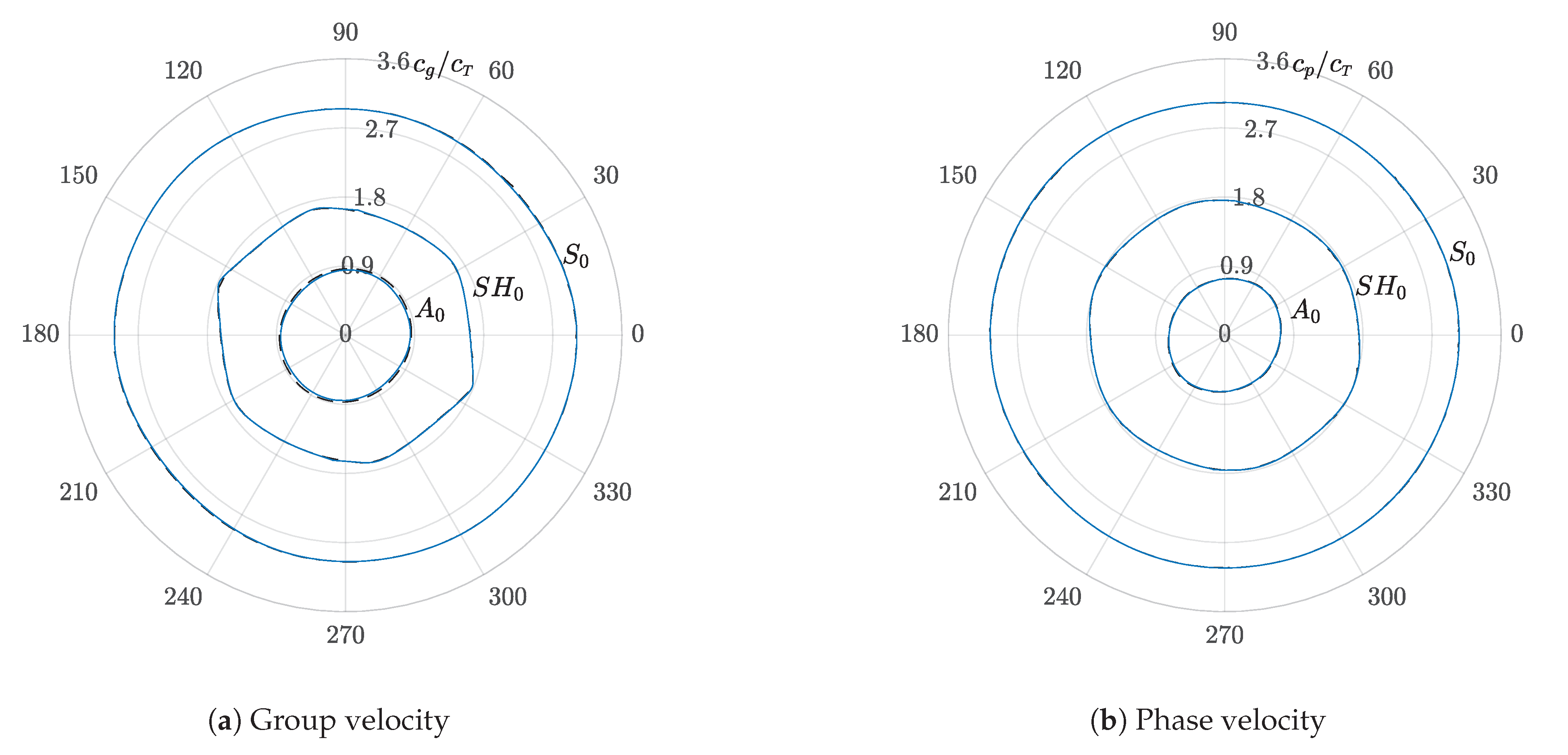
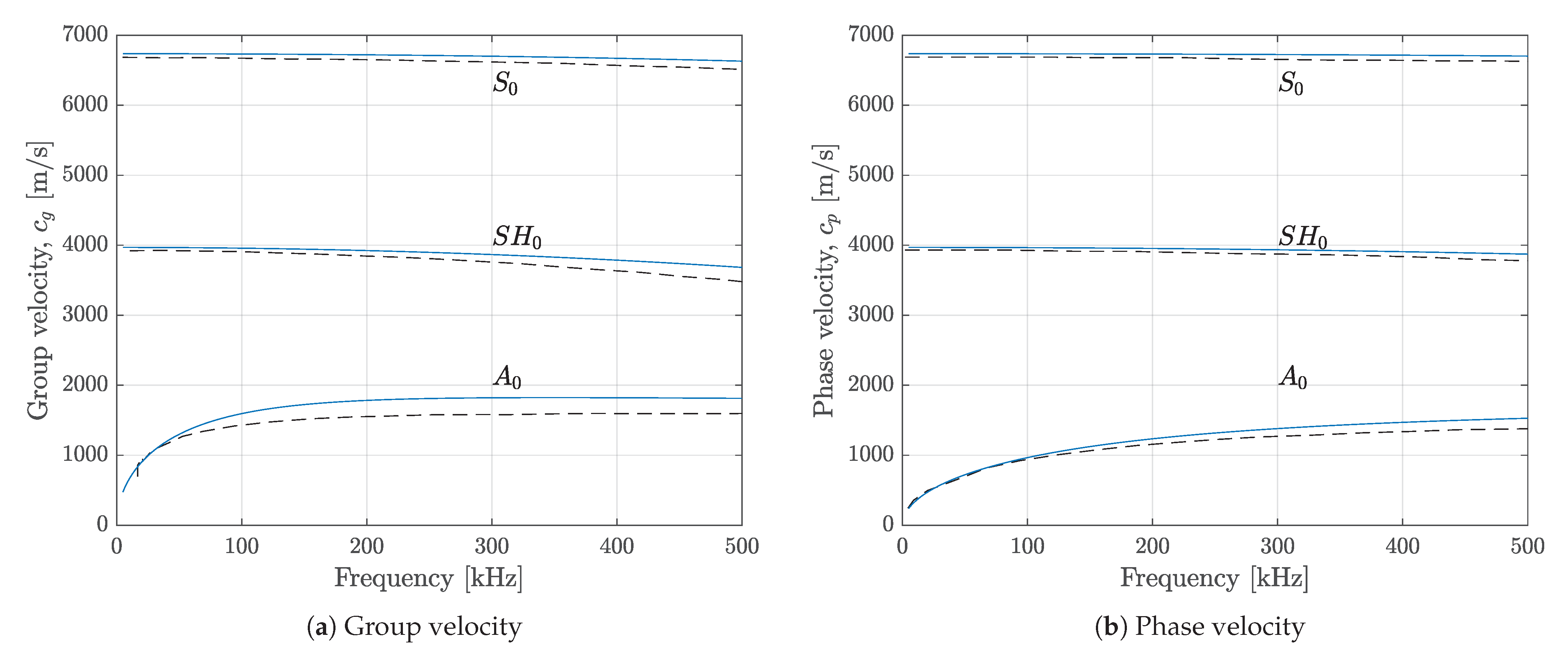
2.3. Velocity Dispersion Curves

The main contribution of this paper is Algorithm 1, which is presented in this section, for obtaining group velocity dispersion curves for periodic structures without finite differentiation using a WFE scheme. The algorithm starts following the basic steps of WFE method, where a periodic section of the structure is modelled in FE software and the $\mathbf{K},\mathbf{M}$, and $\mathbf{C}$ matrices are extracted. They are used to calculate the transfer matrix $\mathfrak{T}$ and obtain its eigenvalues and eigenvectors.

Algorithm 1: Group and phase velocity calculation

In the while loop starting on line 4, the reduction is performed as shown in Equation (2). The variable $k_y$ is initially assigned zero for a point in the $k_x-k_y$ plane lying on the positive $x-$axis ($\theta =0^{\circ }$). The value of $k_y$ is updated in subsequent iterations of the while loop by a suitable step size $\Delta k_y$, such that the polar angle between two consecutive points is less than a desired angular resolution $\Delta \theta$. At each step, $\theta$ is calculated for a particular wave mode by the wavenumbers of that mode using the relation $\theta ={tan}^{-1}(k_y/k_x)$. Note that sorting and identifying a single mode may be difficult especially if a number of propagating modes exist at the excitation frequency. Normally, a modal assurance criterion (MAC) [33] is used to identify modes that can be used here, or a more advanced technique such as the partial wave method presented in [34]. Since a single mode is used for calculating $\theta$, the algorithm can only be used to extract one mode at a time. The same algorithm can easily be extended to filter multiple modes but that is not presented here. The mode shape vector ${\mathit{\varphi }}_x$ is then used to calculate the $x-$component of group velocity $c_{g,x}\left(\theta \right)$. The loop runs until $\theta \ge {\theta }_{max}$, where ${\theta }_{max}$ is slightly below ${90}^{\circ }$. This essentially means that we are looking for part of the dispersion curve that lies in the first quadrant (i.e., between $0{}^{\circ }$ and $90{}^{\circ }$). The reason for stopping before reaching $90{}^{\circ }$ is the asymptotic behaviour of the tangent function at that angle, which makes it numerically difficult to compute. The exact value at $90{}^{\circ }$ is computed later in the algorithm to bypass this issue.

The part of the algorithm discussed so far is used for calculating the $x-$component of the group velocity. To compute the actual group velocity $c_g\left(\theta \right)$ of the mode, $c_{g,y}\left(\theta \right)$ must also be calculated. We find that the ground work for the $y-$component has already been completed. The first zero is appended to the array ${\mathbf{k}}_x$ to compute $k_y$ corresponding to 90 ${}^{\circ }$. It is important to understand that $k_x$ is zero at this angle. Then, a for loop is executed, which iterates through each element of ${\mathbf{k}}_x$. This time, the reduction is performed such that ${\mathbf{q}}_{red}={\left\{{\mathbf{q}}_{lb}^{\mathrm{T}}{\mathbf{q}}_{lt}^{\mathrm{T}}{\mathbf{q}}_l^{\mathrm{T}}\right\}}^{\mathrm{T}}$. The entries of the transformation matrix are modified based on the new ${\mathbf{q}}_{red}$ and now depend on the propagation constant ${\lambda }_x$, as all the degrees of freedom are being projected on the nodes lying on the $y-$axis of the waveguide. The wave mode shape ${\mathit{\varphi }}_y$ is the main unknown quantity that needs to be computed. After that, the calculation of $c_{g,y}\left(\theta \right)$ follows straightforwardly from Equations (6)–(9). Thereafter, the group and phase velocity profiles in the first quadrant are given by:

$$c_g\left(\theta \right)=\sqrt{{\left(c_{g,x}\left(\theta \right)\right)}^2+{\left(c_{g,y}\left(\theta \right)\right)}^2},c_p\left(\theta \right)=\frac{\omega }{k\left(\theta \right)}\mathrm{where}k\left(\theta \right)=\sqrt{{\left(k_x\left(\theta \right)\right)}^2+{\left(k_y\left(\theta \right)\right)}^2}.$$

(10)

The next step is to obtain the velocity profile in the quadrant of 270${}^{\circ }$ to 360${}^{\circ }$. The same algorithm is used to calculate the group velocity profile using the prior knowledge that $k_y\le 0$ in this quadrant. Hence, the step size $\Delta k_y$ becomes negative. The rest of the steps for calculating the velocity profile remain the same as for the first quadrant. This essentially leads to the complete 360${}^{\circ }$ profile by realising that the remaining two quadrants are mirror images (i.e., the profile in quadrant 180${}^{\circ }$ to 270${}^{\circ }$ is a mirror image of the profile in quadrant 0${}^{\circ }$ to 90${}^{\circ }$ and the profile in quadrant 90${}^{\circ }$ to 180${}^{\circ }$ is a mirror image of the profile in quadrant 270${}^{\circ }$ to 360${}^{\circ }$).

3. Comparison with the Literature

The characteristic dispersion curves are important quantities needed for any guided wave application. Therefore, numerous methods have been developed over the years to calculate them. They range from purely analytical methods to purely numerical methods. In this section, the WFE-based method is compared with the most popular existing techniques for the calculation of dispersion curves, and its main advantages are highlighted. All the comparisons were performed against results that have been already published. Notably, none of these methods can be applied to truly periodic structures. The periodic sections for WFE were modelled with standard eight-node hexahedral elements with three degrees of freedom per node. They are shown in Figure 2. The layup was modelled by assigning directional material properties to elements through the thickness.

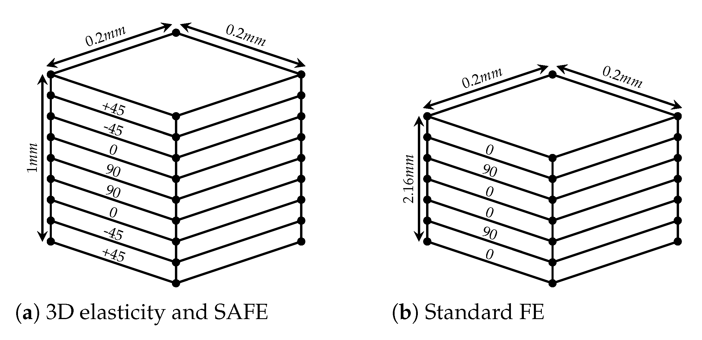
3.1. 3D Elasticity Theory

In this approach [13], the exact dispersion relations are obtained using 3D elasticity theory. The transcendental equations are numerically solved for an infinite number of possible modes. The formulation consists of a robust method to separate symmetric and anti-symmetric modes in symmetric laminates. The wave curves are then obtained by performing the finite difference on the exact solutions of two adjacent slowness surfaces. The results for a 1 mm thick laminate ${[+45/-45/0/90]}_s$ are compared with the WFE scheme in Figure 3, where excellent agreement can be observed. The composite material used in this study was AS4/3502 graphite/epoxy with material properties described in [13]. The material properties were assigned to each layer of the periodic section shown in Figure 2a. The 3D elasticity model is limited to symmetric laminates, whereas the WFE-based approach can handle arbitrary layered structures. Moreover, the solution of transcendental equations is computationally taxing, whereas the developed approach is highly efficient, requiring minimal computational resources with the solution obtained in a fraction of a second.

3.2. Semi-Analytical Finite Element (SAFE) Method

The SAFE method is similar to the WFE scheme, where the finite element method is used for discretising the cross-section of the waveguide [35]. The SAFE method uses a harmonic exponential term to describe the wave behaviour in the propagation direction. The FE discretisation occurs at the cross-section of the waveguide. For plane wave propagation in a plate, a 1D discretisation across the thickness of the plate is sufficient. Combining the harmonic assumption and FE discretisation, the particle displacements are expressed in terms of shape functions. Custom stiffness matrices are assembled using this representation, which are used to set up an eigenvalue problem for the frequency-dependent wavenumber calculation [36]. WFE has a major advantage as it is set up using standard stiffness and mass matrices and no custom formulation is required. Moreover, SAFE cannot be used to model the dispersion characteristics of periodic structures such as the one shown in Figure 1b. The SAFE and WFE models are here compared for the 1 mm thick laminate ${[+45/-45/0/90]}_s$ presented in [35]. The composite laminate in this case is composed of unidirectional T800/924 graphite/epoxy laminae with the material properties described in [35]. The WFE model of the periodic section is shown in Figure 2a, which is again modelled with standard eight-node hexahedral elements. The comparison results are shown in Figure 4, where a similar trend is observed in both approaches with a slight difference in the values.

3.3. Standard Finite Element

The standard finite element (FE) method for extracting the dispersion curves consists of performing a series of modal analyses of a representative part of the structure [37,38]. The dispersion relations are obtained by simply changing the length of the representative portion in order to allow the wavelength to change. The mode shapes and corresponding natural frequencies can be obtained by solving eigenvalue problems. Then, the dispersion curves are obtained from the eigensolutions. This method can only be used to extract propagating modes, whereas the WFE methodology is more general as it can extract both the propagating and evanescent modes. The two techniques were compared for a 2.16 mm thick laminate ${[0/90/0]}_s$. The FE model is shown in Figure 5, where a coarse mesh is shown for visual representation. The laminate is modelled with 2D plane strain elements with the plane strain in the z-direction. The element length is 0.09 mm in the propagation direction and four elements per layer through the thickness. The length of the representative part needs to be changed to obtain the result for different wavelengths. The comparison of dispersion curves is shown in Figure 6, where a good agreement can be observed. The WFE periodic section is shown in Figure 2b, which is modelled using standard eight-node hexahedral elements and the composite material properties for each layer is taken from [37]. The WFE periodic section has orders of magnitude fewer degrees of freedom compared with the standard FE approach. Moreover, the standard FE provides discrete output for each wavelength by changing the length of the representative part, whereas a single periodic section is used in WFE, which can be used to extract dispersion curves for a range of frequencies.

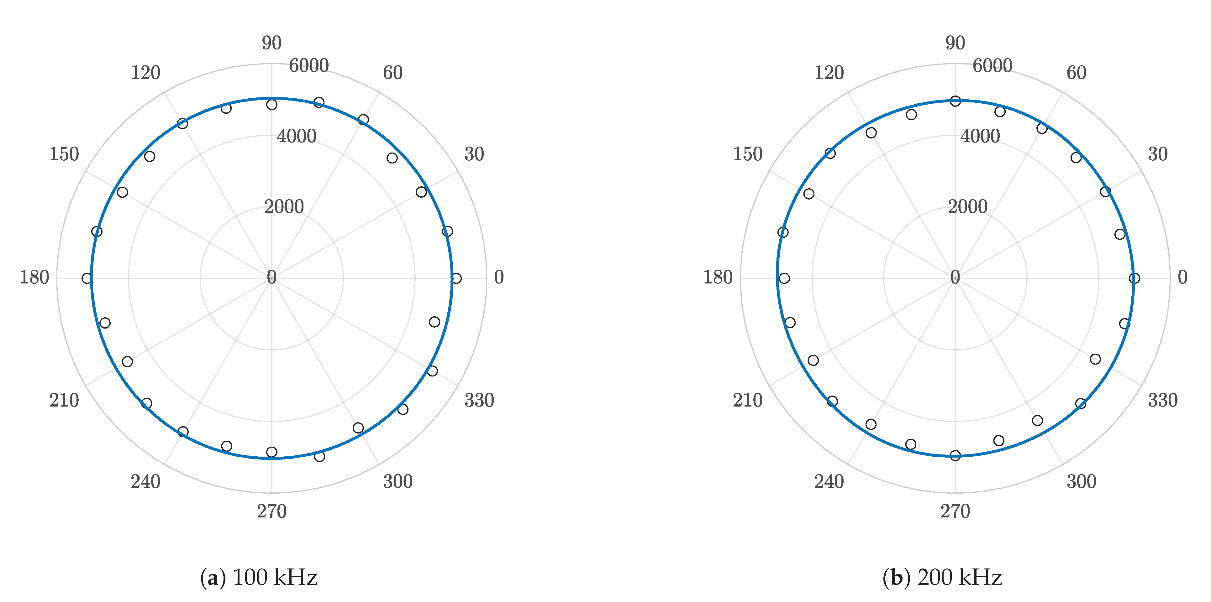
4. Comparison with Experimental Results

In this section, the group velocity computed from WFE is compared with experimentally determined group velocity values for a 2 mm thick CFRP laminate ${[+45/0/-45/90/+45/0/-45/90]}_s$. The composite laminate is composed of unidirectional T800S carbon fibre/epoxy laminae with the material properties described in

Table 2. Material properties of the homogenized CFRP layer (subscript f refers to fibre and m refers to matrix) [39].

Young’s Modulus	Young’s Modulus	Shear Modulus	Shear Modulus	Fibre Volume Fraction	Poisson Ratio	Poisson Ratio	Density
$E_f\left(\mathrm{GPa}\right)$	$E_m\left(\mathrm{GPa}\right)$	$G_f\left(\mathrm{GPa}\right)$	$G_m\left(\mathrm{GPa}\right)$	$V_f$	${\nu }_f$	${\nu }_m$	$\rho (\mathrm{kg}/{\mathrm{m}}^3)$
220	$4.7$	15	$1.85$	$0.4$	$0.2$	$0.3$	1500

. The dimension of the plate is 200 by 200 mm.

The excitation signal was generated from the TG5011 waveform generator and amplified by the Ciprian amplifier. The pulse generator settings were set to a single cycle sine burst centred at 100 kHz for the first test (Figure 7) and 200 kHz for the second test. The experimental setup is shown in Figure 8. The output of the amplifier was split using a T-junction. One output was directed toward the excitation piezoelectric transducer, while the other was attached to the Picoscope signal acquisition system to act as a trigger. The second transducer was also connected to the Picoscope, which received the signal with a sampling frequency of 10 MS/s. All the data were stored in a laptop with the Picoscope 6 program installed. The waves were excited from the centre of the plate and received on a circular boundary 50 mm from the central point of excitation, as shown in Figure 8a. The circular boundary had sensing points in 15${}^{\circ }$ intervals. The group velocity for the fastest wave mode at this frequency (i.e., S₀) was calculated by the time of flight (ToF) method. The ToF of the S₀ wave was determined by measuring the difference between the time the signal was transmitted and received by the transducer. The ToF and and known distance were used to calculate the velocity of the wave at that given point. The tests were repeated 10 times and the average values were computed. The pointwise difference between simulation and experimental data was calculated and found to be less than 5% for all observation points. The results are shown in Figure 9. Notably, the experimental approach used in this research is the simplest method to calculate the group velocity and is limited to the fundamental S${}_0$ mode. More advanced techniques are available that can robustly capture higher-order modes such as the one presented in [13]. The WFE model is also an idealisation of the physical specimen, which might have inherent manufacturing flaws, which is common for composite structures but is not represented in the FE model. Despite these challenges, the experimental and numerical results were found to be in good agreement.

5. Discussion

The proposed WFE-based group velocity calculation technique was described and compared with existing techniques. The model is computationally efficient and can be used for plate-like structures of arbitrary complexity. However, the model is limited by the periodicity assumption in the plane of the plate and hence cannot model variation in cross-section geometry. Moreover, the material properties must also remain consistent in the plane. The WFE scheme also depends on the use of a FE modeller and cannot exist as a standalone platform [40]. The computational efficiency of the model is also reduced in the case of a highly complex single periodic section, which might warrant a further model reduction strategy. In case of a large number of degrees of freedom in a single periodic section, further postprocessing is required to identify and separate propagating and evanescent modes.

6. Conclusions and Outlook

This work presented a new approach for the direct calculation of group velocity curves using the WFE scheme. The WFE scheme was used to exploit the periodicity of the structure to extract the group and phase velocity curves from a representative periodic section. A comprehensive algorithm for calculating the velocity profiles was also constructed. Since the technique is based on FE method, it contains all the uncertainty associated with numerical modelling. This includes the effect of mesh size, element formulation, and model description. In this regard, all the standard best practices of FE modelling should be followed. Moreover, the accuracy of the results will only be as accurate as the model. In case of complex composite structures that have inherent manufacturing flaws, the results will always have uncertainty due to the model definition of the periodic section. Nevertheless, all modelling approaches face similar challenges. The method was compared with existing dispersion curve calculation techniques by comparing the results for complex multi-layered structures. A number of advantages were highlighted with respect to the existing techniques, which are summarised here:

• The technique is easy to implement using the standard FE method without the need for custom formulations.
• It is capable of calculating dispersion properties for arbitrary layered plate-like structures.
• The periodic section is modelled with very few elements, which makes it highly efficient and computationally cheap.
• The theory of the WFE method enables the technique to be used for truly periodic structures, such as textile composites, which cannot be modelled with any existing technique.

Considering the strengths of this approach, it can be used in all guided wave application areas such as material characterisation, non-destructive testing, SHM, etc. It is especially useful in the NDE of aerospace structures, which are fabricated with layered composites and textile composites. It provides a suitable alternative to existing techniques while having the potential to hande more complex structures such as textile composites.

References

1. Dienel, C.P.; Meyer, H.; Werwer, M.; Willberg, C. Estimation of airframe weight reduction by integration of piezoelectric and guided wave–based structural health monitoring. Struct. Health Monit. 2019, 18, 1778–1788. [Google Scholar] [CrossRef] [Green Version]
2. Büyüköztürk, O. Imaging of concrete structures. NDT E Int. 1998, 31, 233–243. [Google Scholar] [CrossRef]
3. Giurgiutiu, V. Structural Health Monitoring of Aerospace Composites; Academic Press: Oxford, UK, 2015. [Google Scholar]
4. Helifa, B.; Oulhadj, A.; Benbelghit, A.; Lefkaier, I.; Boubenider, F.; Boutassouna, D. Detection and measurement of surface cracks in ferromagnetic materials using eddy current testing. NDT E Int. 2006, 39, 384–390. [Google Scholar] [CrossRef]
5. Krautkramer, J.; Krautkramer, H. Ultrasonic Testing of Materials, 4th ed.; Springer: Berlin, Germany, 1990. [Google Scholar]
6. Talreja, R.; Singh, C.V. Damage and Failure of Composite Materials; Cambridge University Press: Cambridge, UK, 2012. [Google Scholar]
7. Banerjee, S.; Ricci, F.; Monaco, E.; Mal, A. A wave propagation and vibration-based approach for damage identification in structural components. J. Sound Vib. 2009, 322, 167–183. [Google Scholar] [CrossRef]
8. Gangadharan, R.; Mahapatra, D.R.; Gopalakrishnan, S.; Murthy, C.; Bhat, M. On the sensitivity of elastic waves due to structural damages: Time–frequency based indexing method. J. Sound Vib. 2009, 320, 915–941. [Google Scholar] [CrossRef]
9. Aggelis, D.; Matikas, T. Effect of plate wave dispersion on the acoustic emission parameters in metals. Comput. Struct. 2012, 98, 17–22. [Google Scholar] [CrossRef]
10. Farrar, C.; Worden, K. Structural Health Monitoring: A Machine Learning Perspective; John Wiley and Sons: New York, NY, USA, 2012. [Google Scholar]
11. Cantero-Chinchilla, S.; Chiachío, J.; Chiachío, M.; Chronopoulos, D.; Jones, A. A robust Bayesian methodology for damage localization in plate-like structures using ultrasonic guided-waves. Mech. Syst. Signal Process. 2019, 122, 192–205. [Google Scholar] [CrossRef] [Green Version]
12. Shen, Y.; Giurgiutiu, V. Effective non-reflective boundary for Lamb waves: Theory, finite element implementation, and applications. Wave Motion 2015, 58, 22–41. [Google Scholar] [CrossRef] [Green Version]
13. Wang, L.; Yuan, F. Group velocity and characteristic wave curves of Lamb waves in composites: Modeling and experiments. Compos. Sci. Technol. 2007, 67, 1370–1384. [Google Scholar] [CrossRef]
14. Nayfeh, A.H.; Chimenti, D.E. Free Wave Propagation in Plates of General Anisotropic Media. J. Appl. Mech. 1989, 56, 881–886. [Google Scholar] [CrossRef] [Green Version]
15. Nayfeh, A.H. The general problem of elastic wave propagation in multilayered anisotropic media. J. Acoust. Soc. Am. 1991, 89, 1521–1531. [Google Scholar] [CrossRef]
16. Moon, F.C. Wave surfaces due to impact on anisotropic plates. J. Compos. Mater. 1972, 6, 62–79. [Google Scholar] [CrossRef]
17. Whitney, J.; Sun, C. A higher order theory for extensional motion of laminated composites. J. Sound Vib. 1973, 30, 85–97. [Google Scholar] [CrossRef]
18. Hakoda, C.; Lissenden, C.J. Application of a general expression for the group velocity vector of elastodynamic guided waves. J. Sound Vib. 2020, 469, 115165. [Google Scholar] [CrossRef]
19. Ahmad, Z.; Vivar-Perez, J.M.; Gabbert, U. Semi-analytical finite element method for modeling of lamb wave propagation. CEAS Aeronaut. J. 2013, 4, 21–33. [Google Scholar] [CrossRef]
20. Thierry, V.; Brown, L.; Chronopoulos, D. Multi-scale wave propagation modelling for two-dimensional periodic textile composites. Compos. Part B Eng. 2018, 150, 144–156. [Google Scholar] [CrossRef] [Green Version]
21. Gravenkamp, H.; Birk, C.; Song, C. Simulation of elastic guided waves interacting with defects in arbitrarily long structures using the scaled boundary finite element method. J. Comput. Phys. 2015, 295, 438–455. [Google Scholar] [CrossRef]
22. Mace, B.R.; Manconi, E. Modelling wave propagation in two-dimensional structures using finite element analysis. J. Sound Vib. 2008, 318, 884–902. [Google Scholar] [CrossRef]
23. Chronopoulos, D.; Droz, C.; Apalowo, R.; Ichchou, M.; Yan, W. Accurate structural identification for layered composite structures, through a wave and finite element scheme. Compos. Struct. 2017, 182, 566–578. [Google Scholar] [CrossRef] [Green Version]
24. Apalowo, R.; Chronopoulos, D.; Tanner, G. Wave Interaction with Defects in Pressurised Composite Structures. J. Nondestruct. Eval. 2018, 37, 48. [Google Scholar] [CrossRef] [Green Version]
25. Malik, M.K.; Chronopoulos, D.; Tanner, G. Transient ultrasonic guided wave simulation in layered composite structures using a hybrid wave and finite element scheme. Compos. Struct. 2020, 246, 112376. [Google Scholar] [CrossRef]
26. Chronopoulos, D. Wave steering effects in anisotropic composite structures: Direct calculation of the energy skew angle through a finite element scheme. Ultrasonics 2017, 73, 43–48. [Google Scholar] [CrossRef] [Green Version]
27. Aly, N.M. A review on utilization of textile composites in transportation towards sustainability. In IOP Conference Series: Materials Science and Engineering; IOP Publishing: Bristol, UK, 2017; Volume 254, p. 042002. [Google Scholar]
28. Mitrou, G.; Ferguson, N.; Renno, J. Wave transmission through two-dimensional structures by the hybrid FE/WFE approach. J. Sound Vib. 2017, 389, 484–501. [Google Scholar] [CrossRef] [Green Version]
29. Waki, Y.; Mace, B.; Brennan, M. Numerical issues concerning the wave and finite element method for free and forced vibrations of waveguides. J. Sound Vib. 2009, 327, 92–108. [Google Scholar] [CrossRef]
30. Renno, J.M.; Mace, B.R. Calculation of reflection and transmission coefficients of joints using a hybrid finite element/wave and finite element approach. J. Sound Vib. 2013, 332, 2149–2164. [Google Scholar] [CrossRef]
31. Mace, B.R.; Duhamel, D.; Brennan, M.J.; Hinke, L. Finite element prediction of wave motion in structural waveguides. J. Acoust. Soc. Am. 2005, 117, 2835–2843. [Google Scholar] [CrossRef]
32. Zhong, W.; Williams, F. On the direct solution of wave propagation for repetitive structures. J. Sound Vib. 1995, 181, 485–501. [Google Scholar] [CrossRef]
33. Allemang, R.J. The modal assurance criterion—Twenty years of use and abuse. Sound Vib. 2003, 37, 14–23. [Google Scholar]
34. Hakoda, C.; Lissenden, C.J. Using the partial wave method for mode-sorting of elastodynamic guided waves. In AIP Conference Proceedings; AIP Publishing LLC: New York, NY, USA, 2019; Volume 2102, p. 020014. [Google Scholar]
35. Bartoli, I.; Marzani, A.; Di Scalea, F.L.; Viola, E. Modeling wave propagation in damped waveguides of arbitrary cross-section. J. Sound Vib. 2006, 295, 685–707. [Google Scholar] [CrossRef]
36. Rose, J.L. Ultrasonic Guided Waves in Solid Media; Cambridge University Press: Cambridge, UK, 2014. [Google Scholar] [CrossRef]
37. Sorohan, Ş.; Constantin, N.; Găvan, M.; Anghel, V. Extraction of dispersion curves for waves propagating in free complex waveguides by standard finite element codes. Ultrasonics 2011, 51, 503–515. [Google Scholar] [CrossRef] [PubMed]
38. Åberg, M.; Gudmundson, P. The usage of standard finite element codes for computation of dispersion relations in materials with periodic microstructure. J. Acoust. Soc. Am. 1997, 102, 2007–2013. [Google Scholar] [CrossRef]
39. Taupin, L.; Lhémery, A.; Inquiété, G. A detailed study of guided wave propagation in a viscoelastic multilayered anisotropic plate. In Journal of Physics: Conference Series; IOP Publishing: Bristol, UK, 2011; Volume 269, p. 012002. [Google Scholar]
40. Cantero-Chinchilla, S.; Malik, M.K.; Chronopoulos, D.; Chiachío, J. Bayesian damage localization and identification based on a transient wave propagation model for composite beam structures. Compos. Struct. 2021, 267, 113849. [Google Scholar] [CrossRef]
Figure 1. Example of a multi-layered 2D periodic structure and discretised FE model of a single periodic section.
Applsci 11 04319 g001
Figure 2. Single periodic section modelled in FE using standard 8-node hexahedral elements.
Applsci 11 04319 g002
Figure 3. Wave velocity curves at 551 kHz for [ + 45 / 45 / 0 / 90 ] s laminate obtained using the analytical (- -) and WFE (–) method.
Applsci 11 04319 g003
Figure 4. Dispersion curves along the principal direction 1 of 0 lamina for [ + 45 / 45 / 0 / 90 ] s laminate obtained using the SAFE (- -) and WFE (–) methods.
Applsci 11 04319 g004
Figure 5. Representative part of laminate modelled in FE.
Applsci 11 04319 g005
Figure 6. Dispersion curves along the principal direction 1 of 0 lamina for [ 0 / 90 / 0 ] s laminate obtained using the FE (- -) and WFE (–) methods.
Applsci 11 04319 g006
Figure 7. Single cycle sine burst excitation signal centred at 100 kHz.
Applsci 11 04319 g007
Figure 8. The experimental setup used for determining the group velocity in a composite plate.
Applsci 11 04319 g008
Figure 9. Group velocity curves for [ + 45 / 0 / 45 / 90 / + 45 / 0 / 45 / 90 ] s laminate from experiments (o) and the WFE (–) method.
Applsci 11 04319 g009