Article

Smooth Design of 3D Self-Supporting Topologies Using Additive Manufacturing Filter and SEMDOT

1
School of Engineering, Deakin University, Waurn Ponds, VIC 3217, Australia
2
Department of Materials Science and Engineering, Monash University, Clayton, VIC 3800, Australia
*
Author to whom correspondence should be addressed.
Appl. Sci. 2021, 11(1), 238; https://doi.org/10.3390/app11010238
Submission received: 2 December 2020 / Revised: 23 December 2020 / Accepted: 24 December 2020 / Published: 29 December 2020
(This article belongs to the Special Issue Design for Additive Manufacturing: Methods and Tools)

Abstract

:
The smooth design of self-supporting topologies has attracted great attention in the design for additive manufacturing (DfAM) field as it cannot only enhance the manufacturability of optimized designs but can obtain light-weight designs that satisfy specific performance requirements. This paper integrates Langelaar’s AM filter into the Smooth-Edged Material Distribution for Optimizing Topology (SEMDOT) algorithm—a new element-based topology optimization method capable of forming smooth boundaries—to obtain print-ready designs without introducing post-processing methods for smoothing boundaries before fabrication and adding extra support structures during fabrication. The effects of different build orientations and critical overhang angles on self-supporting topologies are demonstrated by solving several compliance minimization (stiffness maximization) problems. In addition, a typical compliant mechanism design problem—the force inverter design—is solved to further demonstrate the effectiveness of the combination between SEMDOT and Langelaar’s AM filter.

1. Introduction

Design for additive manufacturing (DfAM) represents a range of design methods through which performance and/or other key considerations such as manufacturability, reliability and cost can be optimized subject to the capabilities of additive manufacturing (AM) technologies [1,2,3,4]. In recent years, topology optimization for AM has become one of the most important branches in DfAM, as topology optimization has great potential to fully exploit the significant benefits provided by the increased design freedom offered by AM [5,6].
As traditional element-based algorithms such as solid isotropic material with penalization (SIMP), rational material with penalization (RAMP) and bi-directional evolutionary structural optimization (BESO) will inevitably form non-smooth boundaries, post-processing or redesign methods have to be used to obtain accurate boundary information for the purpose of engineering applications [7,8,9], meaning that extra efforts have to be made after topology optimization. Given the significance of accurate boundary representation, some element-based algorithms that are capable of forming smooth boundaries such as multiresolution topology optimization (MTO) methods [10,11,12], elemental volume fraction-based methods [13,14,15,16] and a method using floating projection [17,18] have been developed in recent years.
Optimized topologies are fabricated layer-by-layer and have to be sufficiently supported to prevent the component distortion caused by high bending stresses in some AM technologies such as fused deposition modeling (FDM) and selective laser melting (SLM). Even though introducing support structures to topological designs can resolve this issue, more materials need to be wasted, and extra efforts have to be made to remove support structures after manufacturing [19,20,21]. Therefore, optimizing self-supporting topologies directly is an effective way to mitigate overhang angle limitations, save materials and avoid additional effort. Even though there are a great number of investigations regarding 2D self-supporting topologies [22,23,24], these studies have more theoretical value than application value compared to the investigations on 3D self-supporting designs. Studies on 3D self-supporting design have attracted scholarly attention in recent years. The early work in this field was Langelaar’s gradient-based AM filter [25], followed by an improved method capable of executing simultaneous topology optimization and support structures considering metal AM constraints and post-print machining requirements [26]. Han et al. [27] proposed hybrid additive–subtractive manufacturing constraints for 3D continuum structures based on BESO. Mezzadri and Qian [28] proposed a second-order measure of boundary oscillations for overhang control to enhance the manufacturability of designs in AM, and a 3D cantilever beam case was tested. Zhao et al. [29] formulated the self-supporting requirements as an explicit quadratic continuous constraint, and 3D benchmark problems were tested. Zhang and Chen [30] integrated the proposed constraint that was imposed on the overhang angle, directional-dependent overhang angle and horizontal minimum length scale into the MTOP method to conduct the smooth design of 3D self-supporting topologies. van de Ven et al. [31] presented a 3D front propagation-based overhang filter through which printable topologies can be obtained. Most recently, Bi et al. [32] developed a new layer-wise geometric self-supporting constraint for 3D continuum structures based on BESO, and an AM experiment was conducted to validate the effectiveness of the proposed constraint by printing a hinge frame used in the aerospace field.
The authors of this study merely focused on the smooth design of 2D self-supporting topologies through the combination of the Smooth-Edged Material Distribution for Optimizing Topology (SEMDOT) algorithm and Langelaar’s AM filter in previous works [33,34]. Most recently, the authors presented a simple 3D self-supporting case using the Optimality Criteria (OC) optimizer in [35]. In this paper, the smooth design of 3D self-supporting topologies is shown in detail.
The remainder of this paper is structured as follows. Section 2 mathematically demonstrates the combination of SEMDOT and Langelaar’s AM filter. Section 3 presents some numerical experiments to demonstrate the effectiveness and generality of this combination. Finally, conclusions are summarized in Section 4.

2. Integrating Langelaar’s AM Filter into SEMDOT

2.1. Problem Statement

This study uses SEMDOT as an optimization platform to form smooth topologies and Langelaar’s AM filter to obtain 3D self-supporting designs. SEMDOT is a new topology optimization platform that was developed by the authors [16], and its effectiveness has been thoroughly validated. For more details on the advantages of SEMDOT compared to some existing algorithms that are capable of generating smooth boundaries, see [15,16]. Langelaar’s AM filter is a well-established restriction method that can be used with gradient-based topology optimization algorithms, and it has become one of the most extensively used methods for generating self-supporting designs in this community. In SEMDOT, the elemental volume fraction used in the Finite Element Analysis (FEA) model is defined as
X e = 1 N g = 1 N ρ e , g
where N is the total number of grid points in each element and ρ e , g is the density of the gth grid point in the eth element.
The filtering scheme selected in this study is
X ˜ e = l = 1 N e ω e l X l l = 1 N e ω e l
where X ˜ e is the filtered elemental volume fraction, N e is the neighborhood set of elements within the filter domain for the eth element that is a circle centered at the centroid of this element with a predefined filter radius r min , and ω e l is a linear weight factor defined as
ω e l = max ( 0 , r min Δ ( e , l ) )
where Δ ( e , l ) is the center-to-center distance of the lth element within the filter domain to the eth element.
Filtered elemental volume fractions are updated for the next round of FEA by summing up the grid points for each element:
X ˜ e n e w = 1 N g = 1 N ρ e , g n e w
where ρ e , g n e w is the density of the grid point obtained by the Heaviside smooth function.
The relationship between X ˜ e and X ˜ e n e w can be established as
δ e = X ˜ e n e w X ˜ e
where δ e is the deviation of the eth element before and after the update. A detailed discussion of this relationship is presented in [16].
The basic idea of Langelaar’s AM filter is that the value of the element to be supported should not be less than the maximum value of the elements in the supporting region. Figure 1 schematically demonstrates the method of generating self-supporting designs, where the blue element is the element to be supported and the five green elements ( S ( i , j , k ) ) form the supporting region. Mathematical expressions of the 3D Langelaar’s AM filter [25] are given by
ξ ( i , j , k ) = min ( X ˜ ( i , j , k ) , Ξ ( i , j , k ) )       with
Ξ ( i , j , k ) = max ( ξ ( i 1 , j , k 1 ) , ξ ( i , j 1 , k 1 ) , ξ ( i , j , k 1 ) , ξ ( i , j + 1 , k 1 ) , ξ ( i + 1 , j , k 1 ) )
where ξ is the vector of printed elemental volume fractions, X ˜ is the vector of filtered elemental volume fractions and Ξ is the vector of the maximum printed elemental volume fractions.
According to [5,25], the following approximation is made for gradient-based optimization:
ξ = 1 2 X ˜ + Ξ X ˜ Ξ 2 + ε 1 2 + ε
where ε is the parameter that controls the accuracy of the approximation.
The softmax function is used to calculate the maximum value of the elements in the supporting region instead of the P-Q max function in origianl Langelaar’s AM filter [36]. This is because the P-Q max function will generally cause a higher absolute error (the difference between real maximum and maximum smooth approximation) than the softmax function. The softmax function is expressed as defined by Barroqueiro et al. [36]:
smax ( ξ k ) = Ξ ( ξ k ) = k = 1 n s ξ k e P ξ k k = 1 n s e P ξ k
where ξ k is the printed elemental volume fraction in the supporting region relevant to the considered element, P is the parameter that controls the smoothness of the approximation ( 10 4 ), and n s is the number of elements in the supporting region (for 3D cases, n s = 5).

2.2. Topology Optimization Problems

Two typical topology optimization problems: compliance minimization and compliant mechanism design problems are considered in this study. The mathematical statement of compliance minimization design is
min :   C ( X e ) = f T u subject     to :     K ( X e ) u = f e = 1 M X e V e e = 1 M V e V * 0 0 < ρ min X e 1 ;   e = 1 , 2 , , M
where C is compliance; f and u are the global force and displacement vectors, respectively; K is the global stiffness matrix; V e is the volume of the eth element; V * is the prescribed value of the allowable volume; M is the total number of elements; and ρ min is a small artificial parameter, 0.001.
The compliant mechanism design problem is stated as
min :   C ( X e ) = L T u = u o u t subject     to :     K ( X e ) u = f i N e = 1 M X e V e e = 1 M V e V * 0 0 < ρ min X e 1 ;   e = 1 , 2 , , M
where L is a unit length vector with zeros at all degrees of freedom except at the output point, where it is one; u o u t is the output port displacement; and f i N is the input force vector.

2.3. Sensitivity Analysis

Sensitivity analysis measures the effectiveness of changing the elemental volume fractions on the objective function in order to determine the search direction [37,38]. The sensitivity of C p ( ξ ) with respect to X (the vector of elemental volume fractions) is calculated with the chain rule as
C p ( ξ ) X = C p ( ξ ) ξ ξ X ˜ n ew X ˜ n ew X ˜ X ˜ X
Given the discussions of the relationship between X ˜ e and X ˜ e n e w in [16], it can be assumed that ξ n ew / ξ = 1 in this paper for simplicity. The sensitivity of C p ( ξ ) with respect to X ˜ can be calculated based on the derivation of adjoint sensitivity analysis as [5]:
C p ( ξ ) X ˜ j = λ j T ξ j X ˜ j
where λ j is the adjoint field, defined as [5]
λ j T = C p ( ξ ) ξ j + λ j + 1 T λ j + 1 λ j ,       for       1 < = j < N i λ N i T = C p ( ξ ) ξ N i
The remaining derivatives required for executing the sensitivity analysis are calculated as [36]
ξ X ˜ = 1 2 1 X ˜ Ξ X ˜ Ξ 2 + ε 1 2
ξ Ξ = 1 2 1 + X ˜ Ξ X ˜ Ξ 2 + ε 1 2
Ξ k i ξ k = e P ξ k k i = 1 N s e P ξ k i [ 1 + P ( ξ k Ξ ) ]
For more details on the combination of SEMDOT and Langelaar’s AM filter, see the work presented in [33,34]. As the authors’ previous works regarding smooth self-supporting topologies [33,34] were based on the very initial version of SEMDOT, we therefore also refer readers to the paper about the latest version of SEMDOT [16] for further reference.

3. Numerical Experiments

The 3D Matlab code of SEMDOT was developed based on the codes presented by the authors [16] and Liu and Tovar [39], and the 3D Matlab code of Langelaar’s AM filter was developed based on the 2D code provided by Langelaar [5]. Several benchmark optimization problems are solved to validate the effectiveness of the combination of SEMDOT and Langelaar’s AM filter. Parameters in the SEMDOT algorithm are set as presented in [15]. An isotropic linear elastic material model is assumed with a Young’s modulus of 1 MPa and Poisson’s ratio of 0.3 for all examples. A grid with 5 × 5 × 5 points in each element is used to maintain a proper balance between the smoothness of boundaries and computational cost. Unless otherwise stated, the prescribed value of the allowable volume V * is set to 0.3, meaning that 30% of materials within the design domain will be retained; the filter radius r min is set to 1.5 time elements width ( r min = 1.5), a dimensionless size; and the critical overhang angle is set to 45 ° in Langelaar’s AM filter. In addition, the maximum number of iterations is set to 500. The method of moving asymptotes (MMA) proposed by Svanberg [40] is used as the optimizer. Default parameters in MMA are adopted for compliance minimization design, and the move limit is set to 0.05 for compliant mechanism design to improve the convergence stability.

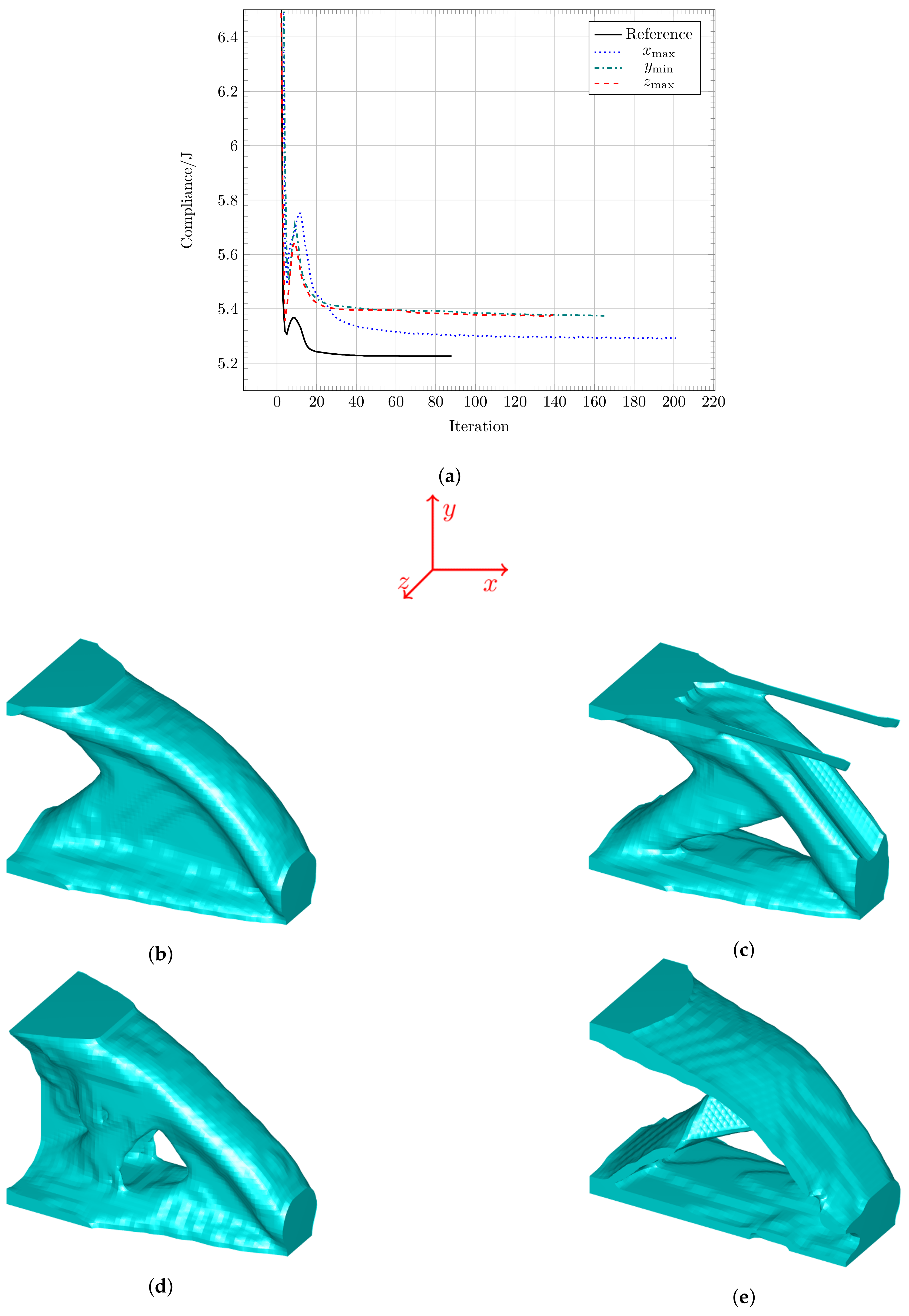
3.1. Different Build Orientations

A deep cantilever beam shown in Figure 2 is considered to demonstrate the influences of different build orientations on compliance, the number of iterations and topologies. In AM, the build orientation is the accumulating orientation of materials when building the part [41]. As illustrated in Figure 2, the left end is fixed and a unit vertical load ( F y = 1 N—Figure 2) is imposed in the middle of the lower edge on the free end. In this study, three build orientations— x max , y min and z max —are considered (see Figure 2). The design domain is discretized by a 60 × 40 × 30 finite element mesh.
Figure 3a shows the reference design case, which converges at 5.226 J after 88 iterations; the optimized topology with the build orientation x max converges at 5.292 J after 201 iterations; the optimized topology with the build orientation y min converges at 5.374 J after 165 iterations; and the optimized topology with the build orientation z max converges at 5.378 J after 139 iterations. It is noted that the reference case is the topological design obtained without using Langelaar’s AM filter (i.e., general topology optimization), and J (N·mm) denotes the multiplication of the force (N) by displacement (mm). Performance sacrifices of 1.25 %, 2.83 %, and 2.91 % are made to form self-supporting designs for build orientations x max , y min and z max , respectively. Even though the self-supporting design in the build orientation y min (Figure 3d) is the most similar to the reference design (Figure 3b), the self-supporting design in the build orientation x max (Figure 3c) is the closest to the reference design in terms of performance. The self-supporting design in the build orientation z max (Figure 3e) obtains the worst performance, as great changes have to be made for this specific direction.

3.2. Different Target Volume Fractions

A simply supported deep beam, as shown in Figure 4, is used to investigate the effects of different target volume fractions on compliance, the number of iterations and topologies. As illustrated in Figure 4, four bottom corners are prevented, and a unit vertical load ( F y = 1 N—Figure 4) is applied in the middle of the top surface. Six different target volume fractions (i.e., 0.15, 0.2, 0.3, 0.4, 0.5 and 0.6) are considered in this study. The design domain is discretized by a 60 × 40 × 20 finite element mesh.
Figure 5a shows that with an increase in the target volume fraction, the performance of optimized topologies gradually imroves, and there are some difficulties in convergence when small target volume fractions ( V * = 0.15 and V * = 0.2 ) are considered. Optimized topologies with different target volume fractions are shown in Figure 5b–g. There is a thin feature in the middle of the optimized topology, as shown in Figure 5b. The value of the element at the bottom of this thin feature is small, whereas elements above this bottom element have greater values, which violates the basic strategy of Langelaar’s AM filter. The formation of this thin feature is because of the absolute error caused by the softmax function (mentioned in Section 2.1).
The first solution to solve this specific thin feature issue is to introduce the weighting factor of w * to the location of element X 3 in the supporting region (see Figure 1). Equation (7) is therefore rewritten as
Ξ ( i , j , k ) = max ( ξ ( i 1 , j , k 1 ) , ξ ( i , j 1 , k 1 ) , w * ξ ( i , j , k 1 ) , ξ ( i , j + 1 , k 1 ) , ξ ( i + 1 , j , k 1 ) )
The related equations are accordingly changed.
The reference design (Figure 6a) converges at 3.621 J after 86 iterations. For the rest of the self-supporting designs (Figure 6b–d), the maximum number of iterations (500) is reached. Among self-supporting designs, the use of a higher weighting factor w * will generally contribute to relatively improved performance. More importantly, the thin feature issue in Figure 5b has been solved by introducing the weighting factor w * , as illustrated in Figure 6b–d.
Another solution is to use a fine mesh, as it can provide more design freedom. The mesh size of 90 × 60 × 30 is used as an example. As the element size is scaled with a certain ratio, the filter radius is scaled with the same ratio to make sure its absolute value remains constant. Figure 7a shows that the self-supporting design case with the fine mesh for V * = 0.15 converges at 3.484 J after reaching the maximum number of iterations (500), and the topological boundary error gradually decreases to almost 0% when the converged topology is obtained. The performance of the fine mesh case is 4.32% better than that of the optimized topology in Figure 5b (3.641 J). Figure 7b shows a much better self-supporting design than that in Figure 5b in terms of manufacturability. There is almost no structural resemblance between coarse mesh (Figure 5b) and fine mesh cases (Figure 7b) as Langelaar’s AM filter is highly mesh-dependent. Compared to the strategy of introducing the weighting factor w * , using the fine mesh is a more general way to solve the thin feature issue.

3.3. Different Critical Overhang Angles

When Langelaar’s AM filter is integrated into traditional element-based algorithms such as SIMP, the critical overhang angle is fixed at 45 ° because of the defined element layout (see Figure 1). As intermediate elements can be cut during the formation of smooth boundaries in SEMDOT, the possibility of exploring different critical overhang angles is therefore provided by the combination of Langelaar’s AM filter and SEMDOT. To obtain self-supporting topologies with different critical overhang angles, the weighting factor of w s = 1 / tan α is introduced to the locations of elements X 1 , X 2 , X 4 , and X 5 in the supporting region (refer to Figure 1) where α is the critical overhang angle. Equation (7) is therefore rewritten as
Ξ ( i , j , k ) = max ( w s ξ ( i 1 , j , k 1 ) , w s ξ ( i , j 1 , k 1 ) , ξ ( i , j , k 1 ) , w s ξ ( i , j + 1 , k 1 ) , w s ξ ( i + 1 , j , k 1 ) )
The related equations are accordingly changed.
Following Section 3.2, a simply supported deep beam with a finite element mesh of 30 × 20 × 20 is used to explore self-supporting topologies with different critical overhang angles (i.e., 30 ° , 45 ° and 60 ° ). The objective function value is multiplied by a scale factor of 100.
Figure 8a shows that the reference design case converges at 326.4 J after 83 iterations, and self-supporting design cases with different critical overhang angles of 30 ° , 45 ° , and 60 ° converge at 328.4 J after 133 iterations, 328.7 J after 109 iterations and 332.2 J after 261 iterations, respectively. Generally, a higher critical overhang angle will cause worse performance as it provides less design freedom. Based on the results presented in Figure 8a, the critical overhang angle of 45 ° requires the least number of iterations to converge among self-supporting design cases. The optimized reference topology is shown in Figure 8b, and optimized topologies with different critical overhang angles are shown in Figure 8c–e.
It should be acknowledged that the mentioned strategy of exploring different critical overhang angles is not suitable for all test cases. For some specific cases, numerical issues may occur during the optimization process, resulting in improper self-supporting designs.

3.4. Force Inverter Design

The force inverter design problem is demonstrated in Figure 9 where an input load is defined in the positive direction, and symmetric constraints are applied on top and side faces (two pink faces). In the case of force inverter design, the goal is to maximize the negative horizontal output displacement. The design domain is discretized by a 40 × 20 × 5 finite element mesh.
Figure 10a shows that the reference design case converges at 1.195 mm after 131 iterations, and the self-supporting design case converges at 1.105 mm after 287 iterations. That is, a performance sacrifice of 7.53% is made to form the self-supporting topology suitable for AM. Compared to the reference topology (Figure 10b), self-supporting features are observed in the optimized topology with Langelaar’s AM filter (Figure 10c).
The compliant mechanism design problem itself is more challenging than the compliance minimization design problem in terms of sensitivity analysis. The problems of self-supporting design for a compliant mechanism in this study demand more accurate sensitivity analysis than general compliant mechanism design problems. Therefore, the successful formation of the self-supporting topology for compliant mechanism design (Figure 10c) further validates the effectiveness of the sensitivity analysis method assumed in SEMDOT. More details on the mentioned sensitivity analysis method can be found in [16].
Based on the results presented from Section 3.1Section 3.4, it can be concluded that the generation of a self-supporting design needs a longer convergence process than its corresponding reference design. The similar phenomenon was also observed by the authors when 2D self-supporting topologies were explored [33,34].

4. Conclusions

This paper integrates Langelaar’s AM filter into SEMDOT—a newly developed element-based algorithm capable of forming smooth boundaries—to implement the smooth design of 3D self-supporting topologies. The obtained conclusions are summarized as follows:
  • The integration of Langelaar’s AM filter in SEMDOT is capable of forming converged 3D self-supporting topologies with smooth boundary representation.
  • As Langelaar’s AM filter is mesh-dependent, the fine mesh is recommended to form proper self-supporting designs when the target volume fraction is small.
  • Different critical overhang angles can be explored using the combination of Langelaar’s AM filter and SEMDOT.
  • The effectiveness of the sensitivity analysis method adopted in SEMDOT is further validated using a 3D compliant mechanism design problem for self-supporting design.
As overhang angle and length constraints interact to determine buildability, the overhang length constraint should be considered in terms of obtaining self-supporting designs in the future. In addition, the experimental validation of the 3D self-supporting topologies obtained using the combination of Langelaar’s AM filter and SEMDOT is required.

Author Contributions

Conceptualization, Y.-F.F., K.G., B.R., Y.W. and L.N.S.C.; methodology, Y.-F.F., K.G., B.R., Y.W. and L.N.S.C.; software, Y.-F.F.; validation, K.G., B.R., Y.W. and L.N.S.C.; formal analysis, Y.-F.F.; investigation, Y.-F.F.; resources, B.R.; writing—original draft preparation, Y.-F.F.; writing—review and editing, K.G., B.R., Y.W. and L.N.S.C.; visualization, Y.-F.F.; supervision, K.G., B.R., Y.W. and L.N.S.C.; project administration, K.G. All authors have read and agreed to the published version of the manuscript.

Funding

This research received no external funding.

Institutional Review Board Statement

Not applicable.

Informed Consent Statement

Not applicable.

Data Availability Statement

The data presented in this study are available on request from the corresponding author. The data are not publicly available due to privacy restriction.

Acknowledgments

The authors would like to thank Krister Svanberg for providing the MMA optimizer code. Yun-Fei Fu would like to thank Matthijs Langelaar, Delft University of Technology, for his invaluable guidance on his 3D AM filter, and Bruno Barroqueiro, University of Aveiro, for his help with the softmax approximation function.

Conflicts of Interest

The authors declare no conflict of interest.

References

  1. Thompson, M.K.; Moroni, G.; Vaneker, T.; Fadel, G.; Campbell, R.I.; Gibson, I.; Bernard, A.; Schulz, J.; Graf, P.; Ahuja, B.; et al. Design for additive manufacturing: Trends, opportunities, considerations, and constraints. CIRP Ann. 2016, 65, 737–760. [Google Scholar] [CrossRef]
  2. Oh, Y.; Zhou, C.; Behdad, S. Part decomposition and assembly-based (Re) design for additive manufacturing: A review. Addit. Manuf. 2018, 22, 230–242. [Google Scholar] [CrossRef]
  3. Izadi, M.; Farzaneh, A.; Mohammed, M.; Gibson, I.; Rolfe, B. A review of laser engineered net shaping (LENS) build and process parameters of metallic parts. Rapid Prototyp. J. 2020, 26, 2228–2236. [Google Scholar] [CrossRef]
  4. Jiang, J.C.; Xiong, Y.; Zhang, Z.Y.; Rosen, D.W. Machine learning integrated design for additive manufacturing. J. Intell. Manuf. 2020, 1–14. [Google Scholar]
  5. Langelaar, M. An additive manufacturing filter for topology optimization of print-ready designs. Struct. Multidiscip. Optim. 2017, 55, 871–883. [Google Scholar] [CrossRef] [Green Version]
  6. Langelaar, M. Combined optimization of part topology, support structure layout and build orientation for additive manufacturing. Struct. Multidiscip. Optim. 2018, 57, 1985–2004. [Google Scholar] [CrossRef] [Green Version]
  7. Ghabraie, K.; Xie, Y.M.; Huang, X.D.; Ren, G. Shape and reinforcement optimization of underground tunnels. J. Comput. Sci. Technol. 2010, 4, 51–63. [Google Scholar] [CrossRef] [Green Version]
  8. Ghabraie, K.; Chan, R.; Huang, X.D.; Xie, Y.M. Shape optimization of metallic yielding devices for passive mitigation of seismic energy. Eng. Struct. 2010, 32, 2258–2267. [Google Scholar] [CrossRef] [Green Version]
  9. Liu, D.D.; Chiu, L.N.S.; Davies, C.; Yan, W. A post-processing method to remove stress singularity and minimize local stress concentration for topology optimized designs. Adv. Eng. Softw. 2020, 145, 102815. [Google Scholar] [CrossRef]
  10. Nguyen, T.H.; Paulino, G.H.; Song, J.; Le, C.H. A computational paradigm for multiresolution topology optimization (MTOP). Struct. Multidiscip. Optim. 2010, 41, 525–539. [Google Scholar] [CrossRef]
  11. Nguyen, T.H.; Paulino, G.H.; Song, J.; Le, C.H. Improving multiresolution topology optimization via multiple discretizations. Int. J. Numer. Methods Eng. 2012, 92, 507–530. [Google Scholar] [CrossRef]
  12. Nguyen, T.H.; Le, C.H.; Hajjar, J.F. Topology optimization using the p-version of the finite element method. Struct. Multidiscip. Optim. 2017, 56, 571–586. [Google Scholar] [CrossRef]
  13. Da, D.C.; Xia, L.; Li, G.Y.; Huang, X.D. Evolutionary topology optimization of continuum structures with smooth boundary representation. Struct. Multidiscip. Optim. 2018, 57, 2143–2159. [Google Scholar] [CrossRef]
  14. Fu, Y.F.; Rolfe, B.; Chiu, N.S.L.; Wang, Y.N.; Huang, X.D.; Ghabraie, K. Topology Optimization of Continuum Structures using Smooth Boundary. In Proceedings of the 13th World Congress on Structural and Multidisciplinary Optimization-Continued, Beijing, China, 20–24 May 2019; pp. 448–454. [Google Scholar]
  15. Fu, Y.F.; Rolfe, B.; Chiu, N.S.L.; Wang, Y.N.; Huang, X.D.; Ghabraie, K. Smooth topological design of 3D continuum structures using elemental volume fractions. Comput. Struct. 2020, 231, 106213. [Google Scholar] [CrossRef]
  16. Fu, Y.F.; Rolfe, B.; Chiu, N.S.L.; Wang, Y.N.; Huang, X.D.; Ghabraie, K. SEMDOT: Smooth-edged material distribution for optimizing topology algorithm. Adv. Eng. Softw. 2020, 150, 102921. [Google Scholar] [CrossRef]
  17. Huang, X.D. Smooth topological design of structures using the floating projection. Eng. Struct. 2020, 208, 110330. [Google Scholar] [CrossRef]
  18. Huang, X.D. On smooth or 0/1 designs of the fixed-mesh element-based topology optimization. Adv. Eng. Softw. 2021, 151, 102942. [Google Scholar] [CrossRef]
  19. Jiang, J.C.; Xu, X.; Stringer, J. Support structures for additive manufacturing: A review. J. Manuf. Mater. Process. 2018, 2, 64. [Google Scholar] [CrossRef] [Green Version]
  20. Jiang, J.C.; Fu, Y.F. A short survey of sustainable material extrusion additive manufacturing. Aust. J. Mech. Eng. 2020, 1–10. [Google Scholar] [CrossRef]
  21. Jiang, J.C. A novel fabrication strategy for additive manufacturing processes. J. Clean. Prod. 2020, 272, 122916. [Google Scholar] [CrossRef]
  22. Liu, J.K.; Gaynor, A.T.; Chen, S.K.; Kang, Z.; Suresh, K.; Takezawa, A.; Li, L.; Kato, J.; Tang, J.Y.; Wang, C.C.; et al. Current and future trends in topology optimization for additive manufacturing. Struct. Multidiscip. Optim. 2018, 57, 2457–2483. [Google Scholar] [CrossRef] [Green Version]
  23. Meng, L.; Zhang, W.; Quan, D.; Shi, G.; Tang, L.; Hou, Y.; Breitkopf, P.; Zhu, J.; Gao, T. From topology optimization design to additive manufacturing: Today’s success and tomorrow’s roadmap. Arch. Comput. Methods Eng. 2020, 27, 805–830. [Google Scholar] [CrossRef]
  24. Fu, Y.F. Recent advances and future trends in exploring Pareto-optimal topologies and additive manufacturing oriented topology optimization. Math. Biosci. Eng. 2020, 17, 4631–4656. [Google Scholar] [CrossRef] [PubMed]
  25. Langelaar, M. Topology optimization of 3D self-supporting structures for additive manufacturing. Addit. Manuf. 2016, 12, 60–70. [Google Scholar] [CrossRef] [Green Version]
  26. Langelaar, M. Integrated component-support topology optimization for additive manufacturing with post-machining. Rapid Prototyp. J. 2019, 25, 255–265. [Google Scholar] [CrossRef] [Green Version]
  27. Han, Y.S.; Xu, B.; Zhao, L.; Xie, Y.M. Topology optimization of continuum structures under hybrid additive-subtractive manufacturing constraints. Struct. Multidiscip. Optim. 2019, 60, 2571–2595. [Google Scholar] [CrossRef]
  28. Mezzadri, F.; Qian, X. A second-order measure of boundary oscillations for overhang control in topology optimization. J. Comput. Phys. 2020, 410, 109365. [Google Scholar] [CrossRef]
  29. Zhao, D.Y.; Li, M.; Liu, Y.S. A novel application framework for self-supporting topology optimization. Vis. Comput. 2020, 1–16. [Google Scholar] [CrossRef]
  30. Zhang, K.Q.; Chen, G.D. Three-dimensional high resolution topology optimization considering additive manufacturing constraints. Addit. Manuf. 2020, 35, 101224. [Google Scholar] [CrossRef]
  31. van de Ven, E.; Maas, R.; Ayas, C.; Langelaar, M.; van Keulen, F. Overhang control based on front propagation in 3D topology optimization for additive manufacturing. Comput. Methods Appl. Mech. Eng. 2020, 369, 113169. [Google Scholar] [CrossRef]
  32. Bi, M.H.; Tran, P.; Xie, Y.M. Topology optimization of 3D continuum structures under geometric self-supporting constraint. Addit. Manuf. 2020, 36, 101422. [Google Scholar]
  33. Fu, Y.F.; Rolfe, B.; Chiu, L.N.S.; Wang, Y.N.; Huang, X.D.; Ghabraie, K. Design and experimental validation of self-supporting topologies for additive manufacturing. Virtual Phys. Prototyp. 2019, 14, 382–394. [Google Scholar] [CrossRef]
  34. Fu, Y.F.; Rolfe, B.; Chiu, L.N.S.; Wang, Y.N.; Huang, X.D.; Ghabraie, K. Parametric studies and manufacturability experiments on smooth self-supporting topologies. Virtual Phys. Prototyp. 2020, 15, 22–34. [Google Scholar] [CrossRef]
  35. Fu, Y.F.; Ghabraie, K.; Rolfe, B.; Wang, Y.N.; Chiu, L.N.S.; Huang, X.D. Optimizing 3D Self-Supporting Topologies for Additive Manufacturing. In Proceedings of the 12th International Conference on Computer Modeling and Simulation, Brisbane, Australia, 22–24 June 2020; pp. 220–223. [Google Scholar]
  36. Barroqueiro, B.; Andrade-Campos, A.; Valente, R.A.F. Designing self supported SLM structures via topology optimization. J. Manuf. Mater. Process. 2019, 3, 68. [Google Scholar] [CrossRef] [Green Version]
  37. Ghabraie, K. The ESO method revisited. Struct. Multidiscip. Optim. 2015, 51, 1211–1222. [Google Scholar] [CrossRef]
  38. Ghabraie, K. An improved soft-kill BESO algorithm for optimal distribution of single or multiple material phases. Struct. Multidiscip. Optim. 2015, 52, 773–790. [Google Scholar] [CrossRef]
  39. Liu, K.; Tovar, A. An efficient 3D topology optimization code written in Matlab. Struct. Multidiscip. Optim. 2014, 50, 1175–1196. [Google Scholar] [CrossRef] [Green Version]
  40. Svanberg, K. The method of moving asymptotes – A new method for structural optimization. Int. J. Numer. Methods Eng. 1987, 24, 359–373. [Google Scholar] [CrossRef]
  41. Qin, Y.C.; Qi, Q.F.; Scott, P.J.; Jiang, X.Q. Determination of optimal build orientation for additive manufacturing using Muirhead mean and prioritised average operators. J. Intell. Manuf. 2019, 30, 3015–3034. [Google Scholar] [CrossRef] [Green Version]
Figure 1. Illustration of the 3D Langelaar’s additive manufacturing (AM) filter [25].
Applsci 11 00238 g001
Figure 2. Design domain of deep cantilever beam.
Applsci 11 00238 g002
Figure 3. Convergence processes and optimized topologies with different build orientations: (a) convergence processes, (b) reference, (c) x max , (d) y min , (e) z max .
Applsci 11 00238 g003
Figure 4. Design domain of a simply supported deep beam.
Applsci 11 00238 g004
Figure 5. Compliance, number of iterations and optimized topologies with different target volume fractions: (a) compliance and number of iterations, (b) V * = 0.15 , (c) V * = 0.2 , (d) V * = 0.03 , (e) V * = 0.4 , (f) V * = 0.5 , (g) V * = 0.6 .
Applsci 11 00238 g005
Figure 6. Optimized topologies with different weighting factors w * : (a) reference, C = 3.621 J. (b) w * = 1.01, C = 3.665 J. (c) w * = 1.015, C = 3.662 J. (d) w * = 1.02, C = 3.659 J.
Applsci 11 00238 g006
Figure 7. Convergence process and optimized topology with a fine mesh for a target volume fraction of 0.15: (a) convergence process, (b) Optimized topology.
Applsci 11 00238 g007
Figure 8. Convergence processes and optimized topologies with different critical overhang angles: (a) convergence processes, (b) reference, (c) 30°, (d) 45°, (e) 60°.
Applsci 11 00238 g008
Figure 9. Design domain of force inverter design.
Applsci 11 00238 g009
Figure 10. Convergence processes and optimized topologies solving the force inverter design case: (a) convergence processes, (b) reference, (c) self-supporting design.
Applsci 11 00238 g010
Publisher’s Note: MDPI stays neutral with regard to jurisdictional claims in published maps and institutional affiliations.

