Remaining Useful Strength (RUS) Prediction of SiC_f-SiC_m Composite Materials Using Deep Learning and Acoustic Emission

Abstract

Prognosis techniques for prediction of remaining useful life (RUL) are of crucial importance to the management of complex systems for they can lead to appropriate maintenance interventions and improvements in reliability. While various data-driven methods have been introduced to predict the remaining useful life (RUL) of machinery systems or batteries, no research has been reported on the remaining useful strength (RUS) prediction of silicon carbide fiber reinforced silicon carbide matrix (SiC_f-SiC_m) materials with pivotal role in its potential usage as a structural material in nuclear reactors and turbine engines. Knowledge of its degradation process is of the utmost importance to the manufacturers. For this purpose, two approaches based on the machine-learning techniques of random-forest (RF) and convolutional neural network (CNN) are proposed to predict the RUS of SiC_f-SiC_m using only acoustic emission (AE) signals generated during the material’s stress applying process. Experimental results show that the CNN models achieved better predictive performance than the RF models but the latter with expert-engineered features achieves better prediction for AE signals in the early stage of degradation. Additionally, our results demonstrate that both models can correctly predict the SiC_f-SiC_m RUS as evaluated by our robust testing method from which the best average root mean square error (RMSE) and Pearson correlation coefficient of 3.55 ksi units and 0.85 were obtained.

1. Introduction

Machinery prognostics have recently emerged as an important research area because of its huge impact on the dependability, durability, and efficiency of complex systems. Lei et al. [1] demonstrated in their review that there has been a considerable increase of machinery prognostics research work between 1997 and 2016. The number of publications between 1997 and 2011 amount to 576 while the total count of publications between 2012 and 2016 is 854. Along with their increasing popularity, there is also an anticipation of those machinery prognostics techniques in the industry [2,3]. Their expected impact is meant to particularly maximize the operational availability, reduce maintenance costs, and improve system reliability and safety [1,2]. An important application of machinery prognostics is the remaining useful life (RUL) prediction: the goal is to predict the time left before observing a failure in a given machine or system [3]. RUL prediction algorithms can be largely grouped into two main categories: data-driven methods and physics-based methods [2]. While requiring a sufficient amount of historical data, the data-driven approaches for prognostics have recently been attracting more attention given their abilities to produce generalizable solutions, which do not require extensive prior knowledge on the physical system [1,2]. In general, data driven approaches need considerable amount of data to train the degradation prediction model of the system of interest [3]. However, thanks to this age of Internet of Things and Industrial 4.0, the great amount of data that is now accessible has made the recent development or adaptation of machine learning-based RUL prediction algorithms possible. Particularly, machine learning techniques have been shown to be capable of learning to predict the RUL of systems given their vibration, sound and other physical signals. Among those machine learning methods, deep learning methods have appeared to be most promising. Deep learning has been demonstrated capable of producing impressive results in areas of computer vision, image and video processing, bioinformatics and natural language processing [4]. Given a sufficient amount of data, deep learning algorithms can build models capable of mapping complex linear or non-linear relationships between input features and output predictions to achieve satisfactory prediction performance [4]. As a result, deep learning has already been increasingly applied to RUL estimation problems [2]. Lei et al. [5] built a model based on a deep fully connected architecture to predict the RUL of rolling bears using both time and frequency domain features. Wu et al. [6] demonstrated that their deep recurrent neural network, their Vanilla Long-Short Term Memory (LSTM) model outperforms other recurrent neural network algorithms for RUL prediction for engineered systems. Based on the convolutional neural network architecture, Babu et al. [7] proposed a novel network with modified convolution and pooling operations to predict RULs.

In this paper, we are interested in one kind of RUL related system degradation monitoring problems: given a component under certain pressure, what additional pressure will lead to its break or fracture. We call this problem as remaining useful strength (RUS) prediction problem. More specifically, we are interested in the degradation prediction problem of SiC_f-SiC_m materials using acoustic emission as the major input signals, which is used in accident tolerant fuel holders in nuclear reactors. This material may degrade over time in their harsh service environments. Thorough knowledge of the deterioration of the SiC_f-SiC_m materials is essential to maintenance of systems built with SiC_f-SiC_m.

SiC_f-SiC_m is a manufactured ceramic composite material that has been researched for its favorable physical attributes [8,9]. Having a high heat tolerance, high irradiation tolerance, good corrosion resistance, good thermal fatigue resistance and desirable toughness, SiC_f-SiC_m materials stand as a potential replacement to the currently used materials in nuclear fuel cladding such as Zircaloys [8,9,10]. SiC_f-SiC_m is a kind of ceramic materials composed of three main components: Silicon carbide fibers, fiber–matrix interphase material and matrix of silicon carbide [11]. In the past, a series of researches have focused on the damage monitoring of the SiC_f-SiC_m components. In their experiments, Truesdale et al. [11] used a non-destructive monitoring technique: the impulse excitation, to investigate the association between signals and the degradation of either one of the SiC_f-SiC_m components. Alva et al. [10] applied multiple tests on tubes of SiC_f-SiC_m materials using the emitted acoustic emission (AE). They showed that the tubes’ degradation undergoes stages, which correspond to the individual degradation of each of the three components. As a materials characterization technique, AE is a well-known non-destructive method that is used in various damage studies of composite materials. During material deterioration, acoustic events in the forms of transient strain waves are emitted [12]. For instance, Whitlow et al. [13] studied the acoustic emission signals to propose a new method to detect and localize damage in continuous ceramic fiber reinforced ceramic matrix composites. Furthermore, Appleby et al. [14] used AE as one of their non-destructive evaluation methods to assess, quantify damage undergone by ceramic matric composites.

In our previous studies [15,16,17], an open-end burst test was carried on nine specimens of SiC_f-SiC_m assembled as tubes. During each burst test, as illustrated in Figure 1, pressure is continuously applied to a tube of SiC_f-SiC_m to simulate stress experimented by the cladding in an accident. As pressure is applied, the cladding keeps getting degraded until it abruptly ruptures. Since the sample is porous and heterogeneous, its failure is a complex accumulation of a great number of microcracking events that involves the cracking of various phases and interface at different geometric scales. In this aspect, the failure process is fundamentally different than the single cracking events in the scratching test as described in [18]. Unlike in homogenous material, the acoustic wave propagation in heterogeneous material with a large number of cracks will be heavily distorted, reflected and attenuated, and are not amenable to analytical treatment. The application of the brutal force machine learning method is thus the better choice here than analytical models. With these said, the most informational characteristics are recorded AE amplitude (event energy), AE duration and hit frequencies. To closely monitor the degradation process, sensors were used to capture the mechanical strain and the emitted AE signals. Additionally, the amount of applied pressure (stress) also gets recorded. Taking our burst tests into consideration, we defined the remaining useful strength (RUS) of the SiC_f-SiC_m as the pressure left to be applied before the tube ruptures.

Following the monitoring process of the SiC_f-SiC_m, more than 40,000 generated AE events were obtained. In light of this amount of AE, we propose three data-driven RUS prediction approaches under the supervised learning framework. Using two machine learning models including random-forest (RF) and convolutional neural networks (CNNs), we build models that learn the correlation between the AE features and the RUS of the material. In the RF based model, we used a select set of descriptive hand-engineered features of the AE while in our CNN based models raw AE signals are used as input for training the CNN prediction models. In our related study [19], we developed a deep learning method to monitor the respective degradation stage of the SiC_f-SiC_m material using the generated AE signals. While our past work led to accurate classification of an AE event into one of three stages, namely, elastic stretching, matrix cracking or fiber cracking, the RUS prediction of an AE event would be more informative and challenging. The predicted RUS of an AE event would yield more insight to the overall degradation process of the SiC_f-SiC_m material since it would indicate the intensity of the deterioration. Even though previous studies did use those aforementioned supervised learning methods on AEs, their application to predict the RUS of SiC_f-SiC_m material is yet to be adapted [19,20], which is done in this work.

As the first implementation of RUS prediction for SiC_f-SiC_m materials, our proposed methods particularly addressed the problem of reusability of tested materials by removing the need to completely rupture the tubes of SiC_f-SiC_m. Furthermore, due to our approach to train and evaluate the models on nine separate sets of AEs from nine experiments, our results reflect the robustness and reliability of our RUS prediction algorithms.

The contributions of this study include the following:

(1)

We use expert-engineered features of AE signals to train a RF model so as to learn the patterns of the generated AE sound events from SiC_f-SiC_m materials for RUS prediction during their degradation.

(2)

We employ the raw AE signals to train two types of end-to-end deep CNN models, thus extracting high-level features from AE events, to achieve better RUS prediction performance and ensure better monitoring of the deterioration process of the test tubes of SiC_f-SiC_m.

(3)

We provide a comprehensive analysis of the models’ performance at predicting the RUS of SiC_f-SiC_m materials based on nine different experiments leading.

2. Materials and Methods

2.1. Dataset

Acoustic signals have been widely used as a mean to closely monitor damages occurring over time in different systems [13,21]. During the mechanical testing in our research, an AE monitoring equipment was used to collect all AE generated during the internal pressurization test of the tubular samples, as described in [10,11]. Physical Acoustics NANO-30 AE sensor with a 125–750 kHz range and a 20 dB preamplifier, the Micro-II Digital AE System, seen in Figure 2, recorded the acoustic events during the internal pressure test. Pressure and strain data were also recorded. As for the SiC composite sample tubes, they are SiGA ^TM composite samples made of nuclear grade fiber, pyrolytic carbon interface coating and CVI SiC matrix that were manufactured and provided by General Atomics.

Each acoustic signal can be represented either as a sound-wave of 3072 values or as 15 expert-designed features. In contrast to the raw representation the acoustic emission signal with 3072 values, the selected features listed in

Table 1. Definition of acoustic emission signal features.

Feature ID	Definition
Feature 1	Rise-Time
Feature 2	Counts
Feature 3	Energy
Feature 4	Duration
Feature 5	Amplitude
Feature 6	Average Frequency
Feature 7	Root Mean square (RMS)
Feature 8	Average Signal Level (ASL)
Feature 9	Counts to Peak
Feature 10	Reverberation Frequency
Feature 11	Initiation Frequency
Feature 12	Signal Strength
Feature 13	Absolute-Energy
Feature 14	Frequency Centroid
Feature 15	Peak Frequency

were calculated by the software operating the burst test. Illustrations of an acoustic emission, along with its occurrence on the strain v. stress plot are displayed in Figure 3 and Figure 4.

From the nine independent degradation tests, 40,140 acoustic events along with their corresponding data were recorded. After removing all AE signals recorded after the tube’s rupture, a total of 39,839 samples remained in our dataset. We defined the RUS value of a given AE signal emitted from a test tube as the difference between the pressure value from that tube’s breaking point (maximum pressure) and that AE’s signal pressure value, which can be defined as in Equation (1):

$$y_{\left(k,i\right)}=\underset{\mathrm{j}}{\max }\left(p_{\left(k,j\right)}\right)-p_{\left(k,i\right)}$$

(1)

where $y$ is the RUS value, $p$ is the pressure value, $k=1, 2,\dots ,9$ is the tube’s index, $i,j=1,2,\dots , n_k$ stand for the acoustic signal’s index within that tube and $n_k$ is the total number of acoustic signals emitted from that tube. Notably, the RUS value for an AE is simply the pressure residual value beyond that AE instance. Figure 5 displays the side-by-side box-and-whisker plots of RUS distribution of the nine separately tested tubes of materials. Additionally,

Table 2. Number of acoustic events recorded per tube until tube’s burst.

Count	Tube #1	Tube #2	Tube #3	Tube #4	Tube #5	Tube #6	Tube #7	Tube #8	Tube #9
AE Events	3286	4978	3869	6126	2893	2674	3590	3504	8919

lists the number of acoustic events recorded per tube. While all the tubes were evaluated in a similar experimental setting, a different number of events was recorded and dissimilar degradation behaviors were observed among all the tests.

To build more robust models and prevent data leakage in our model performance evaluation, we split the original dataset nine times to obtain nine newly separated sets of data, as demonstrated in Figure 6. In each newly created data-set, the testing set consists of all acoustic emission signals belonging to a given ruptured tube and the training set consists of the acoustic emission signals from all the other tubes. For instance, the first created data-set consists of a testing set made up of all AE from tube #1 while the training set contains the signals from the tubes numbered 2 through to 9. Following the initial separation of the training and testing set, the training set was further split by keeping 75% of the data to train the model and 25% as a validation set. We found this tube-level splitting of the dataset was critical for evaluating the generalization and extrapolative prediction capability of our models.

2.2. Methods

Currently, there are two major strategies to achieve high-performance machine learning models. One is to design domain-knowledge based high-quality features combined with standard machine learning algorithms such as random-forest, support vector machines, etc. The other is to take the raw input data and use deep neural network models to build end-to-end learning models by exploiting their hierarchical feature learning capability. Here we chose to develop both types of models using both random-forest and convolutional neural networks and compare their RUS prediction performance.

2.3. Random-Forest

The random-forest (RF) algorithm is a renowned ML technique that was first introduced by Breiman in 2001 [22]. While RF can be used for classification, it can also be used to build powerful regression models. Actually, Wu et al. [23] demonstrated that RF based models achieved the best RUS prediction performance when compared to two other types of ML algorithms. The technique behind RF can be basically summarized into the following two steps:

• The subset of the data used for training will be separated into multiple chunks of data based on the bootstrap aggregation method, which is a technique for separating a data set into multiple subsets in a uniform fashion and with replacement.
• Then for each data chunk, a regression decision tree is built. Then all these trees are combined together to make ensemble predictions.

Upon growing each tree’s nodes through the random splitting of the predictor variables, each decision tree will output a continuous value. Once the trees are fully grown and the model is adequately trained, the values from all the regression trees will be averaged into a single output.

In our work, we trained the same RF model, composed of 100 trees with all the 15 features as described in Table 1.

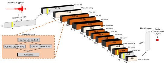
2.4. Convolutional Neural Networks

Convolutional neural networks is one of the most successful deep neural network models, which are specifically designed to consider local information in the input data [4]. Through their successful application, CNN models have been demonstrated capable of producing state-of-the-art results for data with either temporal or spatial relational structure [24]. The implementation of a CNN model leads to the design choices of convolutional layers, the hidden layers, pooling layers, choice of activation functions and finally fully connected layers.

In this work, we proposed two convolutional neural network models for RUS prediction as shown in Figure 7 and Figure 8. Figure 7 shows the first CNN model. The first set of components in our CNN models are the convolutional layers themselves, which discover the inputs’ encoded patterns and then produce a resulting feature map through a series of convolution operations. The mathematical operation of a convolutional filter is illustrated in Figure 9 below with respect to a one-dimensional input. After each convolution layer, a Rectified Linear Unit (ReLU) activation function is inserted, which maps the output from an input layer to a non-linearly transformed output. ReLU, standing for the rectified linear unit, can be defined as a function mapping input values to zero if negative or to the values themselves otherwise, as described in Equation (2).

$$f\left(z\right)=max\left(0,z\right)$$

(2)

Following the convolution layers, pooling layers were added. Through their non-linear down-sampling operations, pooling layers reduced the dimensions of the convolution layer outputs by either taking the average or the maximum values over various local regions within the provided input. Lastly, one or more fully connected layers composed of sequentially arranged neurons produced the predicted RUS output through multiple non-linear transformations.

The first CNN model consists of three convolutional layers and two dense layers. The first convolutional layer used 32 filters of size 9, the second used 64 of size 7 and the last one used 256 of size 5. The number of neurons used by the two fully connected layers were 2304 and 512. Batch-normalization then ReLU activation functions followed each one of the convolutional layers. A drop-out with a rate of 0.3 was applied only to the third convolutional layer.

The general training schema of our CNN models is represented in Figure 10. The loss function used in our CNN models is the root mean square error (RMSE), which is described in Equation (3):

$$RMSE\left(y,\widehat{y}\right)=\sqrt{\frac{1}{n}{\displaystyle \sum }_{i=1}^n{\left(y_i-{\widehat{y}}_i\right)}^2}$$

(3)

where $y$ defines the experimental RUS and $\widehat{y}$ the predicted RUS.

In our second CNN model (Figure 8), we adapted the Squeezenet network [25], which is a deep neural network developed in 2016 with demonstrated success in many computer vision applications. Essentially, the Squeezenet network is composed of sequentially arranged convolutional layers, pooling operations, and blocks of convolutional layers. Each block, named a fire-block, consists of a total of 3 convolutional layers, which efficiently capture the local features of their input. As done in the first version, batch normalization and ReLU activation functions follow each of the convolutional layers within this network. Compared to the standard CNN model in Figure 7, the Squeezenet model has the benefits of a deep architecture for potentially increased accuracy power with significantly less parameters. Additionally, our choice for the Squeeze-Net architecture is also based on its relatively lower computation and parameter storage costs when compared to other more common deep neural architectures.

We trained both CNN models for a maximum of 50 epochs by applying early-stopping with a patience parameter of 10. Additional hyperparameters used in our work consist of a batch size of 40 samples, an initial learning rate of 10⁻³, Glorot uniform weight initialization and the Adam adaptive optimizer. The whole workflow of CNN training can be shown in Figure 10.

3. Results and Discussion

To evaluate the performance of our models, we used metrics of RMSE (Equation (3)) and the Pearson correlation coefficient (R; Equation (4)). The latter describes the linear relationship between two continuous variables in Equation (4) as:

$$R\left(y,\widehat{y}\right)=\frac{{{\displaystyle \sum }}_{i=1}^n\left(y_i-\overline{y}\right)\left(\widehat{y_i}-\overline{\widehat{y}}\right)}{\sqrt{{{\displaystyle \sum }}_{i=1}^n{\left(y_i-\overline{y}\right)}^2}\sqrt{{{\displaystyle \sum }}_{i=1}^n{\left(\widehat{y_i}-\overline{\widehat{y}}\right)}^2}}$$

(4)

where $y$ defines the experimental value and $\widehat{y}$ the predicted RUS value. Overall, the two metrics differ in that the RMSE scores the model’s ability to correctly identify the range in which the predicted RUS resides while R measures the model’s ability to linearly rank the RUS of different AE signals. We used 9-fold cross-validation to evaluate three prediction models in terms of their RUS prediction performance based on AE signals of SiC_f-SiC_m materials:

• Method-1: random-forest model trained with the 15 expert-selected features;
• Method-2: simple standard CNN model trained with the AE signals;
• Method-3: SqueezeNet based model trained with the AE signals.

The RMSE and Pearson correlation coefficient results for each model are reported in

Table 3. Root mean square error (RMSE) of the remaining useful strength (RUS) values as evaluated by 9-fold cross-validation (CV).

Method	Tube #1	Tube #2	Tube #3	Tube #4	Tube #5	Tube #6	Tube #7	Tube #8	Tube #9	Average
RF	3.3	4.03	3.21	3.26	4.99	4.60	2.98	2.33	4.63	3.70
CNN-basic	2.23	4.08	3.3	3.37	5.2	4.07	3.01	2.94	4.15	3.60
CNN-squeeze	2.13	4.09	2.81	3.56	5.51	4.1	3.07	2.64	4.02	3.55

and

Table 4. Pearson correlation (R) as evaluated by 9-fold CV.

Method	Tube #1	Tube 2	Tube #3	Tube #4	Tube #5	Tube #6	Tube #7	Tube #8	Tube #9	Average
RF	0.72	0.81	0.79	0.8	0.82	0.84	0.79	0.93	0.70	0.80
CNN-basic	0.82	0.87	0.85	0.83	0.76	0.83	0.79	0.86	0.81	0.82
CNN-squeeze	0.84	0.9	0.88	0.79	0.79	0.86	0.79	0.87	0.83	0.85

. As expected, there was a clear performance difference between these two types of models when predicting RUS on a given set of AE signals. In regards to the average scores of RMSE and Pearson correlation coefficient R, the CNN models achieved better performance for RUS prediction with their lower average RMSEs of 3.60 and 3.55 compared to 3.70 of RF (last column in Table 3). The CNN models also achieved higher average Pearson correlation coefficient R values of 0.82 and 0.85 compared to 0.80 of RF (last column in Table 4), which means that the predicted remaining stress values to break by the CNN models aligned better with the true values compared to the random forest models. Particularly, between the two types of CNN models, the SqueezeNet model outperformed the standard deep CNN model given that it had the lowest RMSE of 3.55 ksi units and highest R of 0.85. More interestingly, even though the RF algorithm achieved better RMSE results for five out of the nine tubes (tubes numbered 2, 4, 5, 7 and 8), only of three were significantly better (4, 5, 8). On the other hand, the Pearson correlation coefficient results from the convolutional neural network models were higher in nearly all tubes except three tubes (tubes numbered 1, 2, 3, 4, 6 and 9).

Other than the variation by the model architecture, the RUS prediction results also varied amongst the tubes. For tubes numbered 1, 3, 6 and 9, CNN models output RMSE scores that were consistent with the corresponding R values: the highest R values corresponded to the lowest RMSE scores. In contrast, RF outputted consistent results of RMSE and R only in tube 5 and 8. Hence, it was apparent that the models had a challenge at properly mapping AE events distinct to particular tubes to their correct degradation phase. With the knowledge that all of the tubes exhibited different experimental patterns while undergoing the degradation process, we made the assumption that AE signals belonging to different tubes must also differ despite the fact they may have occurred at similar stages of degradation. To verify the assumption, we first categorized a tube’s degradation, with respect to the undergone strain, into 10 stages as defined in Figure 11 and then show the strain stage distribution for all tubes before they broke as shown in Figure 12.

From the RF model outputs, we verified the importance of the features from the model’s training. Out of the 15 features, the uniformly most important feature to RUS prediction is the RMS (root mean square), which is defined as:

$$\mathrm{RMS}=\sqrt{\frac{1}{T_{RMS}}\underset{t_0}{\overset{t_0+T}{{\displaystyle \int }}}U{\left(t\right)}^2}$$

(5)

where U(t) is the acoustic signal.

The average impurity for RMS was 0.61 with a standard deviation of 0.06. Given that RMS is the most representative feature for an AE signal, we inspected how the AE signals from different strain stages differed across various tubes. In Figure 12, we illustrated that the strain distribution undergone by each tube, with respect to strain intensity (stages), was different for all tubes. For example, Tube #4 broke after applying a strain up to stage 4 while Tube #9 shows a much higher strength by holding up to the stage 9 strain before it broke. Additionally,

Table 5. Average RMS of AE in each region by each tube (nan means no values).

Stage #	Tube #1	Tube #2	Tube #3	Tube #4	Tube #5	Tube #6	Tube #7	Tube #8	Tube #9
Stage-1	0.105	0.443	0.224	0.326	0.028	0.108	0.171	0.087	0.047
Stage-2	0.74	1.206	1.14	0.717	0.826	0.652	0.744	1.295	0.587
Stage-3	0.861	1.16	1.094	0.668	0.832	0.512	0.905	0.885	0.932
Stage-4	1.163	0.739	0.706	0.431	0.725	0.807	0.578	0.357	0.638
Stage-5	1.201	0.36	0.411	0.373	0.674	0.775	0.37	0.203	0.532
Stage-6	0.994	0.201	0.338	nan	0.685	0.601	nan	nan	0.317
Stage-7	0.85	0.186	nan	nan	nan	0.471	nan	nan	0.258
Stage-8	0.657	nan	nan	nan	nan	nan	nan	nan	0.165
Stage-9	nan	nan	nan	nan	nan	nan	nan	nan	0.136
Stage-10	nan	nan	nan	nan	nan	nan	nan	nan	0.172

displays the average RMS values for each tube within each stage of strain. It can be found that AE signals from different tubes show high dissimilarity despite the fact that they occurred at similar stages of the degradation. The average RMS of AE signals displayed by the SiC_f-SiC_m tubes were considerably different and they did not present any apparent correlation pattern with the degradation stage. High and low average RMS values were seen throughout the entire testing. With respect to that difference among AE events from different tubes, we could validate the variation in performance of the models across the tubes. For AE events in a testing set, our models will more accurately predict their RUS the less unique these signals were because the models would have already learned their mapping to the degradation space from similar samples. Since the experiments were done in a controlled setting, we attributed the variation of the prediction output from different AEs to the fact that the tested SiC_f-SiC_m assembled tubes were also manufactured with a certain degree of variation. Lastly, there was no apparent correlation between our model performances on RUS prediction and the tubes experimental degradation process of the tubes.

In Figure 13, the predicted and experimental RUS values were plotted against the true pressure values for each testing-set represented by a tube. A mere visualization inspection provided support for our earlier findings. Supporting our results in Table 3, the Squeezenet CNN models generally outperformed other methods. For instance, comparing the different prediction results for tube #1 in Table 2, the RF’s RUS predictions for the AE signals within half-way through the degradation were very poor while the CNN models ranked the AE events linearly in a much better fashion. As for the RMSE results, the models’ performance heavily depended on the individual acoustic signals belonging to a given tube. As previously discussed, a model’s ability to predict an AE’s RUS within a close range of the experimental RUS relies upon the unique features of the AE signal in the feature space. Notably, the following observations could be made:

• The RF model provided a better prediction of RUS for the earliest acoustic emission signals.
• The CNN models generally outperformed the RF model at predicting the RUS for signals, which occurred in the second half of the degradation process.

Therefore, it is clear that the performance of our models depends on the corresponding task for S_iC_f-S_iC_m materials. With the goal of predicting the RUS for a single AE signal that occurs at the early stages of the materials’ degradation, one should use the RF model; otherwise one should apply the CNN models.

4. Conclusions

In this paper, we defined a new type of system prognostic problem, the remaining useful strength (RUS) prediction problem and proposed and developed three machine learning algorithms including random-forest and convolutional neural networks. We applied these algorithms to predict the RUS of the SiC_f-SiC_m tube of materials by employing the AE events from nine burst tubes collected during an internal pressure test. Namely, The RUS is defined as the residual amount of pressure left to rupture an assembled tube of SiC_f-SiC_m. We conducted comprehensive 9-fold cross-validation experiments for training and evaluating our CNN and RF models using the full acoustic emissions signals and their features. We show that while the CNN models on average outperformed the RF model, they present the disadvantage with poor prediction performance in the early stages of the degradation. Additionally, due to the presence of rather unique AE signals in some tubes, the models’ ability at predicting the RUS of an AE depended on the type of tube that an AE belonged to. Our results indicate that AE analysis using state-of-the-art machine learning methods is a reliable and efficient means for monitoring the degradation process of SiC_f-SiC_m materials. In general, using deep convolutional neural networks to extract features from acoustic emission signals is a more robust means to represent the audio samples for predicting their RUS and corresponding stages in the degradation process.

References

1. Lei, Y.; Li, N.; Guo, L.; Li, N.; Yan, T.; Lin, J. Machinery health prognostics: A systematic review from data acquisition to RUL prediction. Mech. Syst. Signal Process. 2018, 104, 799–834. [Google Scholar] [CrossRef]
2. Zhang, A.; Wang, H.; Li, S.; Cui, Y.; Liu, Z.; Yang, G.; Hu, J. Transfer Learning with Deep Recurrent Neural Networks for Remaining Useful Life Estimation. Appl. Sci. 2018, 8, 2416. [Google Scholar] [CrossRef] [Green Version]
3. Jardine, A.K.; Lin, D.; Banjevic, D. A review on machinery diagnostics and prognostics implementing condition-based maintenance. Mech. Syst. Signal Process. 2006, 20, 1483–1510. [Google Scholar] [CrossRef]
4. LeCun, Y.; Bengio, Y.; Hinton, G. Deep learning. Nature 2015, 521, 436–444. [Google Scholar] [CrossRef] [PubMed]
5. Ren, L.; Cui, J.; Sun, Y.; Cheng, X. Multi-bearing remaining useful life collaborative prediction: A deep learning approach. J. Manuf. Syst. 2017, 43, 248–256. [Google Scholar] [CrossRef]
6. Wu, Y.; Yuan, M.; Dong, S.; Lin, L.; Liu, Y. Remaining useful life estimation of engineered systems using vanilla LSTM neural networks. Neurocomputing 2018, 275, 167–179. [Google Scholar] [CrossRef]
7. Babu, G.S.; Zhao, P.; Li, X.-L. Deep convolutional neural network based regression approach for estimation of remaining useful life. In Proceedings of the International Conference on Database Systems for Advanced Applications, Dallas, TX, USA, 16–19 April 2016; Springer: Berlin/Heidelberg, Germany, 2016; pp. 214–228. [Google Scholar]
8. Snead, L.; Nozawa, T.; Ferraris, M.; Katoh, Y.; Shinavski, R.; Sawan, M. Silicon carbide composites as fusion power reactor structural materials. J. Nucl. Mater. 2011, 417, 330–339. [Google Scholar] [CrossRef]
9. Riccardi, B.; Giancarli, L.; Hasegawa, A.; Katoh, Y.; Kohyama, A.; Jones, R.; Snead, L. Issues and advances in SiCf/SiC composites development for fusion reactors. J. Nucl. Mater. 2004, 329, 56–65. [Google Scholar] [CrossRef]
10. Alva, L.H. Monitoring The Progress of Damage in A SICf-SICm Composite Nuclear Fuel Cladding Under Internal Pressure Using Acoustic Emission. Ph.D. Thesis, Department of Mechanical Engineering, University of South Carolina, Columbia, SC, USA, 2018. [Google Scholar]
11. Truesdale, N. Mechanical Characterization and Non-Destructive Evaluation of SiCF-SiCM Composite Tubing with the Impulse Excitation Technique. Ph.D. Thesis, Department of Mechanical Engineering, University of South Carolina, Columbia, SC, USA, 2017. [Google Scholar]
12. Kumar, C.S.; Arumugam, V.; Santulli, C. Characterization of indentation damage resistance of hybrid composite laminates using acoustic emission monitoring. Compos. Part B Eng. 2017, 111, 165–178. [Google Scholar] [CrossRef]
13. Whitlow, T.; Jones, E.; Przybyla, C. In-situ damage monitoring of a SiC/SiC ceramic matrix composite using acoustic emission and digital image correlation. Compos. Struct. 2016, 158, 245–251. [Google Scholar] [CrossRef]
14. Appleby, M.; Zhu, D.; Morscher, G. Mechanical properties and real-time damage evaluations of environmental barrier coated SiC/SiC CMCs subjected to tensile loading under thermal gradients. Surf. Coat. Technol. 2015, 284, 318–326. [Google Scholar] [CrossRef] [Green Version]
15. Alva, L.H.; Huang, X.; Jacobsen, G.M.; Back, C.A. High Pressure Burst Testing of SiC f-SiC m Composite Nuclear Fuel Cladding. In Advancement of Optical Methods in Experimental Mechanics; Springer: Berlin/Heidelberg, Germany, 2015; Volume 3, pp. 387–393. [Google Scholar]
16. Shapovalov, K.; Jacobsen, G.M.; Alva, L.; Truesdale, N.; Deck, C.P.; Huang, X. Strength of SiCf-SiCm composite tube under uniaxial and multiaxial loading. J. Nucl. Mater. 2018, 500, 280–294. [Google Scholar] [CrossRef]
17. Alva, L.; Shapovalov, K.; Jacobsen, G.M.; Back, C.A.; Huang, X. Experimental study of thermo-mechanical behavior of SiC composite tubing under high temperature gradient using solid surrogate. J. Nucl. Mater. 2015, 466, 698–711. [Google Scholar] [CrossRef] [Green Version]
18. Von Stebut, J.; Lapostolle, F.; Bucsa, M.; Vallen, H. Acoustic emission monitoring of single cracking events and associated damage mechanism analysis in indentation and scratch testing. Surf. Coat. Technol. 1999, 116, 160–171. [Google Scholar] [CrossRef]
19. Nasiri, A.; Bao, J.; Mccleeary, D.; Louis, S.-Y.M.; Huang, X.; Hu, J. Online Damage Monitoring of SiC f-SiC m Composite Materials Using Acoustic Emission and Deep Learning. IEEE Access 2019, 7, 140534–140541. [Google Scholar] [CrossRef]
20. Ebrahimkhanlou, A.; Salamone, S. Single-sensor acoustic emission source localization in plate-like structures using deep learning. Aerospace 2018, 5, 50. [Google Scholar] [CrossRef] [Green Version]
21. Elforjani, M.; Shanbr, S. Prognosis of bearing acoustic emission signals using supervised machine learning. IEEE Trans. Ind. Electron. 2017, 65, 5864–5871. [Google Scholar] [CrossRef] [Green Version]
22. Breiman, L. Random forests. Mach. Learn. 2001, 45, 5–32. [Google Scholar] [CrossRef] [Green Version]
23. Wu, D.; Jennings, C.; Terpenny, J.; Gao, R.X.; Kumara, S. A comparative study on machine learning algorithms for smart manufacturing: Tool wear prediction using random forests. J. Manuf. Sci. Eng. 2017, 139, 071018. [Google Scholar] [CrossRef]
24. Piczak, K.J. Environmental sound classification with convolutional neural networks. In Proceedings of the 2015 IEEE 25th International Workshop on Machine Learning for Signal Processing (MLSP), Boston, MA, USA, 17–20 September 2015; pp. 1–6. [Google Scholar]
25. Iandola, F.N.; Han, S.; Moskewicz, M.W.; Ashraf, K.; Dally, W.J.; Keutzer, K. SqueezeNet: AlexNet-level accuracy with 50x fewer parameters and < 0.5 MB model size. arXiv 2016, arXiv:1602.07360. [Google Scholar]
Figure 1. Open end burst test setting on the SiCf-SiCm tubes. (a) Schema of the setting for the burst test. (b) Real experimental setup of the burst test.
Applsci 10 02680 g001
Figure 2. Experimental setup of acoustic emission (AE) equipment used to collect the acoustic events.
Applsci 10 02680 g002
Figure 3. Visualization of the AE signal numbered 3280 emitted from tube #1.
Applsci 10 02680 g003
Figure 4. Strain vs. internal pressure (Ksi) plot from tube #1. In blue: all AE signals within the tube. In red: AE signal numbered 3280. In green: AE from breaking instance numbered 3286.
Applsci 10 02680 g004
Figure 5. Side-by-side box-plots of each RUS distribution from the test on the 9 tubes.
Applsci 10 02680 g005
Figure 6. Illustration of the third created dataset, which is obtained by keeping all AE signals from the third tube in the testing set and AE from all other tubes in the training set.
Applsci 10 02680 g006
Figure 7. Architecture of the basic convolutional neural network (CNN) model.
Applsci 10 02680 g007
Figure 8. Architecture of the SqueezeNet based CNN model.
Applsci 10 02680 g008
Figure 9. Illustration of one-dimensional convolution filter operation.
Applsci 10 02680 g009
Figure 10. Workflow Schema of our CNN models. (a) Normalized Input is a 1-dimensional array of 3072 values. (b) Kernels of 1D-CNN layers convolve over input x. (c) Outputs of 1D-CNN layers are fed to a pooling layer. (d) Subsampled outputs are provided to fully connected layers, which then output a remaining useful strength (RUS) value.
Applsci 10 02680 g010
Figure 11. Description of the 10 stages of a tube’s degradation.
Applsci 10 02680 g011
Figure 12. Bar plot of strain by each tube. Each bar displays the categorization of the 10 strain phases described in Table 4.
Applsci 10 02680 g012
Figure 13. Stress versus RUS plots for each given tube. (a) Random-forest (RF), (b) Basic CNN and (c) SqueezeNet CNN. Blue represents the predicted values while red represents the true values.
Applsci 10 02680 g013